The Evolution of the Galaxy Rest-Frame Ultraviolet Luminosity Function Over the First Two Billion YearsNote: Submitted to the Astrophysical Journal
Abstract
We present a robust measurement and analysis of the rest-frame ultraviolet (UV) luminosity functions at 4 to 8. We use deep Hubble Space Telescope imaging over the CANDELS/GOODS fields, the Hubble Ultra Deep Field and the Hubble Frontier Field deep parallel observations near the Abell 2744 and MACS J0416.1-2403 clusters. The combination of these surveys provides an effective volume of 0.6–1.2 106 Mpc3 over this epoch, allowing us to perform a robust search for faint (M18) and bright (M21) high-redshift galaxies. We select candidate galaxies using a well-tested photometric redshift technique with careful screening of contaminants, finding a sample of 7446 candidate galaxies at 3.5 8.5, with 1000 galaxies at 6 – 8. We measure both a stepwise luminosity function for candidate galaxies in our redshift samples, as well as a Schechter function, using a Markov Chain Monte Carlo analysis to measure robust uncertainties. At the faint end our UV luminosity functions agree with previous studies, yet we find a higher abundance of UV-bright candidate galaxies at 6. Our best-fit value of the characteristic magnitude is consistent with 21 at 5, different than that inferred based on previous trends at lower redshift, and brighter at 2 significance than previous measures at 6 and 7 [20, 24]. At 8, a single power-law provides an equally good fit to the UV luminosity function, while at 6 and 7, an exponential cutoff at the bright end is moderately preferred. We compare our luminosity functions to semi-analytical models, and find that the lack of evolution in is consistent with models where the impact of dust attenuation on the bright end of the luminosity function decreases at higher redshift, though a decreasing impact of feedback may also be possible. We measure the evolution of the cosmic star-formation rate (SFR) density by integrating our observed luminosity functions to M17, correcting for dust attenuation, and find that the SFR density declines proportionally to (1)-4.3±0.5 at 4, consistent with observations at 9. Our observed luminosity functions are consistent with a reionization history that starts at 10, completes at 6, and reaches a midpoint (x 0.5) at 6.7 9.4. Finally, using a constant cumulative number density selection and an empirically derived rising star-formation history, our observations predict that the abundance of bright 9 galaxies is likely higher than previous constraints, though consistent with recent estimates of bright 10 galaxies.
Subject headings
early universe — galaxies: evolution — galaxies: formation — galaxies: high-redshift — ultraviolet: galaxiesI. Introduction
The past half-decade has seen a remarkable increase in our understanding of galaxy evolution over the first billion years after the Big Bang, primarily due to the updated near-infrared capabilities of the Hubble Space Telescope. Robust galaxy samples at 6 now include more than 1000 objects [21, 110, 57, 98, 33, 60, 166, 111, e.g.,] with a few candidate galaxies having likely redshifts as high as 10 [23, 51, 99, 112, 41, 113, 27, e.g.,]. These galaxies are selected photometrically, primarily based on a sharp break at rest-frame 1216 Å due to absorption by intervening neutral hydrogen in the intergalactic medium (IGM).
Studies of galaxies at 6 have revealed a number of interesting results. Galaxies at 6 8 appear to have bluer rest-frame ultraviolet (UV) colors than at lower redshift, likely due to a decrease in dust attenuation, although the brightest/most massive galaxies do appear to have comparable dust attenuation at 4–7 [144, 57, 22, 160, 60, 50, 26, e.g.,]. Lower mass galaxies have colors consistent with stellar populations harboring significant metal content (though likely sub-Solar), and therefore the currently detectable populations of galaxies are not dominated by the primordial first generation of stars [60, 49, 50, e.g.,]. The structures of these galaxies are resolvable, though they show small sizes with half-light radii 1 kpc, consistent with the evolution previously detected at lower redshifts [56, 109, 116, e.g.,]. Finally, the abundance of high-redshift star-forming galaxies may account for the necessary photons to sustain an ionized intergalactic medium (IGM) by 6, and perhaps as high as 7–8 if one assumes that galaxies at least 5 magnitudes below the detection limit of HST exist [59, 128, e.g.,], though the unknown ionizing photon escape fraction is a major systematic uncertainty.
One of the key measurements is the galaxy rest-frame UV luminosity function (hereafter referred to as the luminosity function), as it is one of the most useful tools to study the evolution of a galaxy population. This measure encapsulates the relative abundances of galaxies over a wide dynamic range in luminosity. As the UV light probes recent star-formation activity, the integral of the rest-UV luminosity function provides an estimate of the cosmic star-formation rate density [94, 25, 93, e.g.,], although this measurement is reliant on dust corrections. The luminosity function is typically parameterized with a Schechter [133] function with a power-law slope at faint luminosities, and an exponentially declining form at the bright end. Comparing the shape of the luminosity function to the underlying dark-matter halo mass function, previous studies have found that the luminosity function at 6, when normalized to the halo mass function at the characteristic magnitude , lies below the halo mass function at both bright and faint luminosities. This is generally assumed to be due to feedback: dominated by accreting supermassive black holes at the bright end (active galactic nuclei; AGN), and by supernova or radiative-driven winds at the faint end [143, e.g.,]. Dust extinction can also play a role, particularly if the level of attenuation is dependent on a galaxies stellar mass or UV luminosity [60, 26, e.g.,]. Although luminous AGN are present at 6 [53, e.g.,], they are exceedingly rare, and to date only a single quasar has been observed at 7 [102]. Therefore one may expect the degree of the exponential decline at the bright end to become weaker with increasing redshift. In addition, robustly quantifying the bright end of the luminosity function can allow us to gain physical insight into how these distant galaxies turn their gas into stars, as the star-formation timescale is a significant fraction of the age of the Universe, therefore enough time has not yet elapsed for feedback to bring these galaxies into equilibrium. A change in the star-formation timescale is therefore more readily apparent in the shape of the bright end of the luminosity function [142, e.g.,].
Thanks to the combination of observations from GALEX and the Hubble Space Telescope estimates of the UV luminosity function exist now from 1 [4, 43] out 8 [20, 97, 24, 111, 112, 90, e.g,]. Earlier works have concluded that declines from around 21 at 3 to fainter than 20 at 8, with the faint-end slope becoming steeper over this same redshift range [20, 124, 24, 99, 135, e.g.,]. However, in order to adequately quantify the amplitude and form of the bright end, large volumes need to be probed, as bright sources are relatively rare. This has been accomplished via a combination of ground and space-based surveys at 6, with a variety of studies showing conclusively that a single power law does not fit the data, and that some sort of cut-off is needed at the bright end [4, 20, 124, 97, e.g.,]. Although previous luminosity functions have been published at 6, the space-based studies have been based on small volumes [24, e.g.,], and thus, while they can somewhat constrain the faint-end slope, they do not have the capability to constrain the bright end.
Recent studies are starting to make progress at the bright end. Finkelstein et al. [61], while selecting galaxies for spectroscopic followup in the GOODS-N field, found an overabundance of bright galaxies at 7. Ono et al. [115] found a similar result, with their discovery of the M21.8 galaxy GN-108036 at 7.2 in GOODS-N. Likewise, Hathi et al. [72] found two bright 6.5 candidate galaxies in a ground-based near-infrared survey of GOODS-N. Thus, it appears that the abundance of galaxies at the bright end of the luminosity function may not be decreasing towards higher redshift as previously thought. Although these studies were based in a single field, further evidence comes from Bowler et al. [29], who used new deep ground-based near-infrared imaging from the UltraVISTA survey [96] to discover 34 luminous 7 galaxy candidates over 1.65 deg2. They combined these galaxies with the results from McLure et al. [99], which included deep and wide HST imaging over 300 arcmin2 in the GOODS-S, UDS and HUDF fields, to analyze the rest-frame UV luminosity function at 7. They concluded that they did see evidence for a drop-off in the luminosity function at the bright end, however, the drop-off was less steep than that predicted by a Schechter function, leading them to postulate that the 7 luminosity function has the shape of a double-power law, perhaps similar to that of the possible form of far-infrared luminosity functions [132, 37].
In this study, we measure the rest-frame UV luminosity function at 4 8 with solely space-based data, using the largest HST project ever, the Cosmic Assembly Near-infrared Deep Extragalactic Legacy Survey (CANDELS; PIs Faber & Ferguson). The large area observed by CANDELS allows us to probe large volumes of the distant universe for the rare, bright galaxies. With these data, we investigate the form of the bright end of the luminosity function and the implications on galaxy evolution. In addition to the deep data in the HUDF, we use the CANDELS data in the GOODS-S and GOODS-N fields, which have not only deeper near-infrared imaging, but also imaging in more optical and near-infrared filters than the other three CANDELS fields (UDS, EGS and COSMOS). We also include in our analysis the parallel fields from the first year dataset of the Hubble Frontier Fields, near the Abell 2744 and MACS J0416.1-2403 galaxy clusters. The combination of these data allows us to select a large sample of nearly 7500 galaxies, over a wide dynamic range in UV luminosity at 4–8 (Figure 1).
| Field | Area | |||||||||
|---|---|---|---|---|---|---|---|---|---|---|
| (arcmin2) | (mag) | (mag) | (mag) | (mag) | (mag) | (mag) | (mag) | (mag) | (mag) | |
| GOODS-S Deep | 61.6 | 28.2 | 28.6 | 27.9 | 28.1 | 27.8 | 28.2 | 28.1 | — | 27.9 |
| GOODS-S ERS | 41.4 | 28.2 | 28.5 | 27.9 | 27.9 | 27.6 | 27.6 | 28.0 | — | 27.8 |
| GOODS-S Wide | 35.6 | 28.2 | 28.7 | 28.1 | 27.9 | 27.9 | 27.3 | 27.6 | — | 27.4 |
| GOODS-N Deep | 67.6 | 28.1 | 28.3 | 27.9 | — | 27.7 | 28.1 | 28.3 | — | 28.1 |
| GOODS-N Wide | 71.7 | 28.1 | 28.4 | 27.8 | — | 27.6 | 27.3 | 27.4 | — | 27.4 |
| HUDF Main | 5.1 | 29.5 | 30.0 | 29.7 | — | 29.1 | 29.9 | 29.6 | 29.6 | 29.7 |
| HUDF PAR1 | 4.7 | — | 29.0 | 28.8 | — | 28.5 | 28.9 | 29.0 | — | 28.8 |
| HUDF PAR2 | 4.8 | — | 29.0 | 28.7 | — | 28.3 | 28.9 | 29.2 | — | 28.9 |
| MACS0416 PAR | 4.4 | 28.8 | 28.9 | — | 29.2 | — | 29.2 | 29.0 | 29.0 | 29.0 |
| Abell 2744 PAR | 4.3 | 29.0 | 29.1 | — | 29.2 | — | 29.1 | 28.8 | 28.8 | 28.9 |
| Zeropoints | — | 25.68 | 26.51 | 25.67 | 25.95 | 24.87 | 26.27 | 26.23 | 26.45 | 25.95 |
Note. — The magnitudes quoted are 5 limits measured in 0.4′′-diameter apertures on non-PSF matched images.
This paper is organized as follows. In § 2 we discuss the imaging data used and the catalog construction, and in §3 we present our sample selection via photometric redshifts, and estimates of the contamination. In § 4 we highlight our completeness simulations, and in § 5 we discuss the construction of the rest-UV luminosity function at 4, 5, 6, 7 and 8. In § 6 we discuss the implications of our luminosity function results, while in § 7 we compare our results to semi-analytical models. In § 8 we present our measurements of the cosmic star-formation rate density, and in § 9 we discuss the implications for galaxies at higher redshifts. Our conclusions are presented in § 10. Throughout this paper we assume a WMAP7 cosmology [82], with H 70.2 km s-1 Mpc-1, 0.275, 0.725 and 0.816. All magnitudes given are in the AB system [114]. All error bars shown in the figures represent 1 uncertainties (or central 68% confidence ranges), unless otherwise stated.
II. Observations and Photometry
II.1. Imaging Data
Studying galaxies in the early universe requires extremely deep imaging, necessitating space-based data. Additionally, to probe a large dynamic range in luminosities, we need to combine deep studies over small areas with larger-area surveys with shallower limiting magnitudes. Our study used imaging data from a number of surveys covering both the Northern and Southern fields from the Great Observatories Origins Deep Survey [66], with both the Hubble Space Telescope (HST) and the Spitzer Space Telescope.
The deepest imaging comes from three surveys of the Hubble Ultra Deep Field (HUDF): the original HUDF survey which obtained optical imaging with the Advanced Camera for Surveys [12, ACS;]; and the more recent HUDF09 [21, 110, PI Illingworth; e.g.,] and UDF12 surveys [51, 81, PI Ellis;], which obtained near-infrared imaging with the Wide Field Camera 3 (WFC3). The full HST dataset over the HUDF comprises imaging in eight bands: F435W, F606W, F775W and F850LP with ACS, and F105W, F125W, F140W and F160W with WFC3 (hereafter referred to as , , , , , and , respectively), which cover an area of 5 arcmin2. The HUDF09 survey also obtained deep WFC3 imaging over two similarly-sized flanking fields, first observed with ACS in the UDF05 survey [108, PI Stiavelli;], referred to as the HUDF09-01 and HUDF09-02 fields [24]. These fields each have imaging in the , , , , , and bands.
The majority of our candidate galaxy sample comes from the Cosmic Assembly Near-infrared Deep Extragalactic Legacy Survey [69, 80, CANDELS; PIs Faber and Ferguson;]. CANDELS is the largest HST project ever, comprising 902 orbits over five extragalactic deep fields, including the two GOODS fields [66]. CANDELS, which finished in August 2013, is composed of a deep and a wide survey. The deep survey covers the central 50% of each of the two GOODS fields, while the wide survey covers the remainder of the GOODS-N field, and the southern 25% of the GOODS-S field to depths 1 mag shallower than the deep survey (the wide survey also covers three additional fields not used in this study; see §6.4.1 and Figure 15). We use ACS imaging from the original GOODS survey in the , , and bands. We use the most recent ACS mosaics in these fields, which in GOODS-S includes all ACS imaging in that field prior to the ACS repair on Servicing Mission 4 in 2009, and in the GOODS-N field includes all ACS imaging from the GOODS survey (CANDELS internal team release versions 3 and 2, respectively). The CANDELS imaging in both the deep and wide regions of both GOODS fields includes the , and bands. We add to our GOODS-S dataset imaging over the northern 25% of the GOODS-S field from the WFC3 Science Oversight Committee’s Early Release Science (ERS) program [162, PI O’Connell;], which also includes and imaging, as well as the F098M (hereafter referred to as ) band. Unless otherwise distinguished, throughout the paper we will refer to and together as the -band (both filters probe observed 1m light, but the filter is narrower and thus has a higher spectral resolution).
Finally, we complete our dataset with the recently obtained deep HST observations near the galaxy clusters Abell 2744 and MACS J0416.1-2403 (hereafter MACS0416) from the Hubble Frontier Fields (HFF) program (PI Lotz). For this study, we use only the parallel (unlensed) fields. Both fields have been observed in the , , , , , and bands. We use these data to complement our candidate galaxy samples at 5, 6, 7 and 8 (excluding 4 due to the reduced number of optical bands).
In parallel to the primary WFC3 observations, CANDELS obtained extremely deep imaging in the F814W band (hereafter ) in both of the GOODS fields. As these data were obtained recently, they suffers from poor charge transfer efficiency. Although algorithms have been devised to correct for this [3], as the CANDELS fields have imaging in both the and bands, we do not include the CANDELS photometry in the initial photometric redshift fitting (though we do explore its inclusion in §3.6). However, we did use these very deep data during our visual inspection step, which was highly useful at 8, where true 8 galaxies should be completely undetected in the -band. In the HFF parallel fields, where the band is the only imaging covering the red end of the optical, we used these data in the full analysis.
The description of the CANDELS HST imaging reduction is available from Koekemoer et al. [80]. These reduction steps were also followed for the ERS, HUDF [81] and HFF data we use here. We use imaging mosaics with 0.06′′ pixels, and make use of their associated weight and rms maps. The combined imaging dataset covers an area of 301.2 arcmin2, with 5 limiting magnitudes in the band ranging from 27.4 to 29.7 mag (measured in 0.4′′ diameter apertures). These datasets are summarized in Table 1.
II.2. Point Spread Function Matching
The HST imaging used here spans more than a factor of three in wavelength, thus the differences in point-spread function (PSF) full-width at half-maximum (FWHM) across that range are significant. For example, the PSF in the GOODS-S Deep field has a FWHM 0.193′′ in the -band, but only 0.119′′ in the -band. A point-source will thus have more of its flux contained within a 0.4′′ aperture in the -band compared to the -band. As the selection of distant galaxies relies very heavily on accurate colors, and we are using apertures of fixed sizes (determined by the detection image, see §2.3) to measure photometry in all bands, this changing PSF needs to be addressed.
We corrected for this by matching the PSF of the HST imaging to the -band image (which has the largest PSF FWHM) in each field. We did this using the IDL deconv_tool Lucy-Richardson deconvolution routine, in the same way as Finkelstein et al. [57], Finkelstein et al. [60]. This routine requires the PSF for a given band as well as a reference PSF (in this case, the -band), and it generates a kernel. The PSFs were generated by stacking stars in each field in each band, where the stars were selected via identifying the stellar locus in a half-light radius versus magnitude plane. Each star was then visually inspected to ensure that there were no bright near-neighbors, and then the stars were stacked, subsampling by a factor of 10 to ensure an accurate centroiding of each star (i.e., to avoid smearing the PSF during the stacking). Using these PSFs, the deconvolution routine performed an iterative process, and relies on the user to determine the number of iterations. We did this by making a guess as to the correct number of iterations, and then changing this number until the stars in the PSF-matched images in a given band had curves-of-growth which matched the -band curves-of-growth to within 1% at a radius of 0.4′′. The images were then convolved with the final kernel to generate PSF-matched images.
II.3. Photometry
Photometry was measured on the PSF-matched dataset with a modified version of the Source Extractor software [15, v2.8.6,]. Our modified version adds a buffer between the source and the local background cell and removes spurious sources associated with the distant wings of bright objects. Catalogs were generated independently in each of our ten sub-fields, using Source Extractor in two-image mode, where the same detection image was used to measure photometry from all available HST filters. For most of our fields, we used a weighted sum of the F125W and F160W images as the detection image, to increase our sensitivity to faint objects. In the HUDF main field and the MACS0416 and A2744 HFF parallel fields, we supplemented this catalog with catalogs using 10 additional detection images, derived by stacking all possible combinations of adjacent WFC3 filters. In these three fields, a combined catalog was made up of all unique sources in the catalogs, using a 0.2′′ matching radius. This allowed very blue sources that may be too faint in the image to be selected in the original F125W+F160W-selected catalog to be included. This procedure was replicated in our completeness simulations (§4). To derive accurate flux uncertainties, Source Extractor relies on both an accurate rms map, and a realistic estimate of the effective gain. The provided rms map has been shown to produce accurate uncertainties, and it has been corrected for pixel-to-pixel correlations which occur as a result of the drizzling process [70, see] which are typically on the order of 10 - 15% of the total rms. The effective gains were computed for each band separately as the the instrument gain (1 for ACS, 2.5 for WFC3/IR) the total exposure time for a given image. We have previously verified that the uncertainties measured in this manner on HST imaging are accurate [60]. The zero-points to convert the observed fluxes into AB magnitudes are given in Table 1, and are appropriate for the dates when these data were taken.
Following our previous work [57, 59, 60, 61], colors were measured in small Kron apertures with the Source Extractor Kron aperture parameter PHOT_AUTOPARAMS set to values of 1.2 and 1.7. Finkelstein et al. [60] found that these apertures result in more reliable colors for faint galaxies when compared to isophotal or small circular apertures. An aperture correction to the total flux was derived in the -band and was computed as the ratio between this small Kron aperture flux, and the default Source Extractor MAG_AUTO flux, which is computed with PHOT_AUTOPARAMS 2.5, 3.5. These aperture corrections were then applied to the fluxes in all filters. To see if our aperture corrections accurately recovered the total flux, we examined our completeness simulations (discussed in §4), and found that after applying this aperture correction recovered fluxes were typically 5% fainter in each band than their input fluxes (with the exception of the HUDF main field, where the measured correction was 2%). We thus increased the flux in each band by the appropriate factor to derive our best estimate of the total flux.


The Source Extractor catalogs from each band were combined into a master catalog for each field. At this step, the observed fluxes were corrected for Galactic extinction using the color excess E(B-V) from Schlafly & Finkbeiner [137] appropriate for a given field11 1 http://ned.ipac.caltech.edu/forms/calculator.html, and using the Cardelli et al. [36] Milky Way reddening curve to derive the corrections based on each filter’s central wavelength. We used a mask image to remove objects in regions of bad data, where the mask was generated using a threshold value from the weight map. This mask primarily trims off the noisier edges of the imaging, but it also excludes the “death star” region on the WFC3 array where the number of dithers was low (i.e., in the CANDELS Wide regions). The areas quoted in Table 1 are those of the good regions in these masks. Objects were also removed from the catalog if they had a negative aperture correction, which applied to a very small number of sources, primarily restricted to areas near very bright sources where the flux in the larger aperture was unreliable. The remaining objects comprised our final catalog in each field.
III. Sample Selection
III.1. Photometric Redshifts
We selected our candidate high-redshift galaxy sample via a photometric redshift fitting technique. This has the advantage in that it uses all of the available photometry simultaneously, rather than the multi-step Lyman break galaxy (LBG) method, which selects galaxies using two colors, and then subsequently imposes a set of optical non-detection criteria [20, 24, e.g.,]. Another advantage of photometric redshifts is that one obtains a redshift probability distribution function (PDF), which not only allows one to have a better estimate of the redshift uncertainty ( typically 0.2–0.3 versus 0.5 for the LBG technique), but can also be used as a tool in the construction of the sample itself. A potential disadvantage of photometric redshift techniques is that the results are based on a set of assumed template spectra; if these templates do not encompass properties similar to the galaxies being studying, systematic offsets may occur (though we also note that similar templates are used to construct LBG color selection criteria). That being said, initial work comparing the differences between galaxy samples selected via both LBG and photometric redshift techniques found that the resulting sample properties are fairly similar [99, 135, e.g.,].
Photometric redshifts for all sources in the catalogs for each fields were measured using the EAZY software [30]. The input catalog used all available HST photometry, with the exception of the F814W imaging in the CANDELS fields, which was used solely for visual inspection (see §2.1). We used an updated set of templates provided with EAZY based on the PÉGASE stellar population synthesis models [64], which now include an increased contribution from emission lines, as recent evidence points to strong rest-frame optical emission lines being ubiquitous amongst star-forming galaxy populations at high-redshift [7, 58, 154, 141, 145, 61, e.g.,]. EAZY assumes the intergalactic medium (IGM) prescription of Madau [92]. EAZY does have the option to include magnitude priors when fitting photometric redshifts, which uses the luminosity functions as a prior for whether a galaxy at a given apparent magnitude resides at a given redshift. As we show later, there is still non-negligible uncertainty at the bright end of the luminosity function, therefore we did not include these magnitude priors during our photometric-redshift fitting process.
III.2. Selection Criteria
We selected candidate galaxy samples in five redshift bins centered at 4, 5, 6, 7 and 8 with 1, using criteria similar to our previous work [60, 61]. The cosmic time elapsed between our last two bins at 7 and 8 is 125 Myr. This time is much longer than the dynamical time of the systems we study, and thus leaves significant time for evolution. However, as studies of galaxy evolution move towards higher redshift, this will not always be the case (e.g., 40 Myr) thus future studies with the James Webb Space Telescope will need to pay careful attention to the choice of sample redshifts when studying galaxy evolution.
Rather than relying solely on the best-fit redshift value, we used the full redshift probability distribution curves calculated by EAZY (where exp(), normalized to unity). Our selection criteria are:
-
1) A 3.5 significance detection in both the and bands. A requirement of a significant detection in two bands removes nearly all spurious sources, as the chances of a noise peak occurring in two images at the same position are very small (§3.8.1). This requirement also limits our analysis to galaxies with 8.5, as the Lyman break shifts into the band at 8.1.


Figure 2.— Left) The distribution of photometric redshifts in our candidate galaxy sample. The red shading denotes candidates discovered in the CANDELS GOODS fields (including the ERS), while the blue shading denotes those in the combined five deep fields from the HUDF09 and HFF parallel programs. The shallower yet much wider CANDELS imaging dominate the numbers in every redshift bin, by a factor of 10 at 4–5, and 2 at 7–8, though the deep fields are necessary for constraints on the faint end of the luminosity function. Right) A comparison between the spectroscopic redshift and our best-fit photometric redshifts for the 171 galaxies in our sample with spectroscopic redshifts in the literature. The red circles denote galaxies with 1 at 3 significance. There are only six such galaxies, and all have spectroscopic redshifts at 4. -
2) The integral of the redshift probability distribution function under the primary redshift peak must comprise at least 70% of the total integral. This enforces that no more than 30% of the integrated redshift PDF can be in a secondary redshift solution.
-
3) The integral under the redshift PDF in the redshift corresponding to a given sample (i.e., 6.5 – 7.5 for the 7 sample) must be at least 25%, which ensures that the redshift PDF is not too broad.
-
4) The area under the curve in the redshift range of interest must be higher than the area in any other redshift range (i.e., for a galaxy in the 7 sample, the integral of must be higher than the integral in any other redshift bin). This criterion ensures that a given galaxy cannot be included in more than one redshift sample.
-
5) At least 50% of the redshift PDF must be above (i.e., 0.5 for 7), and the best fit redshift must be above .
-
6) The from the fit must be less than or equal to 60. This criterion ensures that EAZY provides a reasonable fit, though in practice it does not reject many sources.
-
7) Magnitude in the band must be 22. This effectively cleans many stars from our sample, but the limit is still more than two magnitudes brighter than our brightest 6 galaxy candidate. At 4, we do have a few sources close to this limit, but only two sources are brighter than 22.4. This fact, coupled with the observation that the very few sources at 22 that satisfy our 4 selection criteria are either obvious stars, or diffraction spikes, implies that this criterion should not significantly affect our luminosity function results.
Of these criteria, items #1 and #2 are by far the most constraining, as most galaxies which meet these criteria, with 3.5 make it into our sample. Items #3 and #4 are responsible for putting a candidate galaxy in a given redshift sample. While some of the cuts above are arbitrary, these choices will be corrected for as we apply these same criteria to our completeness simulations discussed in §4. In Figure 2 we compare the photometric redshifts for 171 galaxies in our sample to available spectroscopic redshifts in the literature22 2 The spectroscopic redshifts come from a compilation made by N. Hathi (private communication) which include data from the following studies: Szokoly et al. [148], Grazian et al. [67], Vanzella et al. [156], Vanzella et al. [157], Hathi et al. [71], Barger et al. [9], Rhoads et al. [125], Wuyts et al. [163], Balestra et al. [8], Ono et al. [115], Kurk et al. [85], Rhoads et al. [126], Finkelstein et al. [61].. The agreement is excellent, with 0.031 (derived by taking an iterative 3-clipped standard deviation), though the number of confirmed redshifts at 6.5 is small (only five galaxies). The number of outliers is also small, with only six out of 171 galaxies (3.5%) having a photometric redshift differing from the spectroscopic redshift by 1 at 3 significance. All of these six galaxies have 4, thus no galaxies in our sample have a catastrophically lower spectroscopic redshift. In comparison, defining outliers in the same way, we find that the published CANDELS team photometric-redshift catalog has 13 outliers out of 174 total spectroscopic redshifts, for a somewhat higher outlier fraction of 7.5% [45]. Although the fraction of galaxies with confirmed redshifts is relatively small, the available spectroscopy confirms that our selection methods yield an accurate high-redshift sample. In the remainder of this paper, we will therefore refer to our candidate galaxies solely as galaxies, with the caveat that spectroscopic followup of a much larger sample, particularly at 6, is warranted.
III.3. Visual Inspection
As the candidate selection process is automated, for a truly robust galaxy sample, we required a visual inspection of each of our 7500 candidate high-redshift galaxies. During the visual inspection, we examined the following features:

Is the source a real galaxy? Objects were inspected to ensure that they were not an artifact, examples of which are a part of a diffraction spike (which frequently appear in different places in the ACS and WFC3 imaging due to different roll angles during the respective observations), oversplit regions of bright galaxies, or noise near the edge of the images.
Is the aperture drawn correctly? While the small Kron apertures yield the most reliable colors, they are also susceptible to “stretching” (i.e., becoming highly elongated) in regions of high noise or near very bright objects. For each source, we compared the ratio of the flux between the Kron aperture and a 0.4′′-diameter circular aperture to that same quantity for objects of a similar magnitude from the full photometry catalog. If an object had a value 30% higher than similarly bright sources in the full photometry catalog and the aperture looks to have been affected by noise/bright sources, we adjusted the photometry of the object in question accordingly, using the 0.4′′-to-total correction of similarly-bright objects in the catalog. In practice, these issues affected 10% of galaxies in our high-redshift sample.
Is there significant optical flux that did not get measured correctly? Primarily due to the issues with inaccurate apertures discussed in the above bullet, a very small number of sources appeared to have optical flux when visually inspected that was not measured to be significant in our catalog (i.e., in the case of a too-large aperture, the flux is concentrated in a small number of pixels, while the flux error comes from the full aperture, so the signal-to-noise is low). In these cases, objects were removed from our sample. This step is somewhat qualitative, as there are cases of objects where the aperture appears correct, yet there is still a 1–2 detection in a single optical band. In the majority of these cases, as we are confident in our photometric redshift analysis, we left these objects in the sample. During this step, we also examined photometry for each source in the CANDELS fields, which primarily benefits the selection of 8 galaxies, which should not be visible at this wavelength. Three 8 candidates with observable flux were removed from our sample.
III.4. Stellar Contamination
The most crucial step in our visual inspection is the classification and removal of stellar sources, as stellar contamination would dominate the bright end of the luminosity function if these contaminants were not considered. In particular, M-type stars as well as L and T brown dwarf stars can have similar colors (including optical non-detections) as our high-redshift galaxies of interest, particularly at 6. While some studies use dwarf star colors during their selection [28, 99, 29, e.g.,], many use primarily the Source Extractor “stellarity” parameter to diagnose whether a compact object is a star or a galaxy [24, 27, e.g.,]. However, the stellarity parameter loses its ability to discern between a point source and a resolved source for faint objects. To test this further, we examined the stellarity of sources in the CANDELS GOODS catalogs. At very bright magnitudes ( 24), there is a clear separation between stars and galaxies, with objects either having a stellarity near unity (i.e., stars), or having stellarity near zero (i.e., galaxies). However, this separation becomes less clear at 25, where the stellar and galaxy sequences begin to blend together. Therefore, stellarity can be an unreliable star-galaxy separator at 25, which is similar to the brightness of our brightest 7 galaxies.
While the GOODS fields cover relatively small regions on the sky, the potential number of brown dwarf contaminants, even at 25, is significant. The Galactic structure model of Ryan & Reid (in prep) predicts the surface density of brown dwarfs in our covered fields. In the GOODS-S region, using the area covered by the CANDELS, ERS and HUDF09 observations, we would expect 6 stars of spectral type M6–T9 with -band magnitudes between 25 and 27. The surface density of M6-T9 stars in GOODS-N is similar, with an expected number of stars in the field of 5. Thus, the expected number of 25 27 stars of spectral type M6-T9 in our whole surveyed region is 11. While this number is small, the numbers of brown dwarfs are expected to fall off toward fainter magnitudes, thus the majority of these are likely have close to 25. This magnitude is similar to those of the brightest galaxies in our sample, which dominate the shape of the bright end of the galaxy luminosity function. As stellarity is an unreliable method of identifying these sources, we must find an alternative method.
Although brown dwarfs can have similar colors to 6 galaxies, and can be included in the initial sample, they fall on well-defined color sequences, and can thus be distinguished from true galaxies. Figure 3 shows two color-color plots33 3 This research has benefitted from the SpeX Prism Spectral Libraries, maintained by Adam Burgasser at http://pono.ucsd.edu/adam/browndwarfs/spexprism which we used in tandem with the size information, examining not only stellarity, but also the FWHM and half-light radius as measured by Source Extractor, to identify stars lurking our sample (similar plots were used at 4 and 5). If a galaxy appeared un-resolved (defined as having a stellarity 0.8, or a half-light radius and/or FWHM similar to that of stars in the field) then we examined that object in the color-color plots as shown in Figure 3. If the object also had colors similar to a dwarf star, then we removed it from our sample. Over all of our fields, we had a total of 23 objects flagged as stars (many with 25) in our 6 samples; 18 from our initial 6 galaxy sample, and 5 from our initial 7 galaxy sample. These objects were removed from our sample. One of these stars removed from our 7 sample was previously flagged as a probable T-dwarf by Castellano et al. [40]. We examined the subset of eight of these stars which were detected in the FourStar Galaxy Evolution (zFourGE) medium band imaging survey of a portion of GOODS-S, and found that all eight have and colors consistent with brown dwarf stars [][where and refer to two of the three medium bands which comprise the band][149]. Of these, six stars have 25, meaning that our high-redshift galaxy selection criteria also originally selected half of the expected number of faint brown dwarfs in this field. Four of these six stars have Source Extractor stellarity measurements 0.8, thus a stellarity-only rejection method would have failed to remove them. We conclude that our visual inspection step efficiently removed stellar contaminants from our sample, but we emphasize that the color examination portion was crucial to exclude the faintest stars from our sample.
III.5. Active Galactic Nuclei
We screened for the presence of bright active galactic nuclei (AGN) in our sample by searching for counterparts in Chandra X-ray Observatory point source catalogs. In the GOODS-S field, we used the 4 Msec Chandra Deep Field – South (CDF-S) catalog of Xue et al. [164], and in GOODS-N, we used the 2Msec Chandra Deep Field – North catalog of Alexander et al. [2]. These catalogs have average positional accuracies of 0.42′′ and 0.3′′, respectively. To be conservative, we searched for matches in each catalog out to a radius of 1′′. We then visually inspected each of the 34 galaxies in our sample with a match. Seven objects, all with Chandra catalog separations 0.6′′, had nearby HST counterparts with positions consistent with the Chandra catalog, and thus these interlopers are likely providing the X-ray emission; none of these sources had spectroscopic redshifts in the CDF-S catalog. These seven sources thus remained in our sample. The remaining 27 sources, all with separations 0.6 ′′, had Chandra positions consistent with the X-ray emission coming from the galaxies in our sample. Secure spectroscopic redshifts were available for four of these 27 galaxies in the CDF-S catalog, of 3.06, 3.66, 3.70 and 4.76. These 27 galaxies (25 from our 4 sample, and two from our 5 sample) were removed from our galaxy sample. This removal is conservative, as although the X-ray detections imply the presence of an AGN, it does not prove that the AGN dominates the UV luminosity.
III.6. Photometric Redshifts with Spitzer/IRAC Photometry
As we will discuss below, one of the main results of this work is an apparent constant value of at 5, brighter than many previous works. It is thus imperative that we have high confidence that our bright galaxies are all in fact at high-redshift, and not lower-redshift contaminants. To provide a further check on our bright sources, we re-examined the photometric redshifts of our bright galaxies with the addition of Spitzer Space Telescope Infrared Array Camera [55, IRAC;] imaging over our fields. This imaging probes the rest-frame optical at these wavelengths, and thus provides significant constraining power because the most likely contaminants are red, lower-redshift galaxies, which would have very different fluxes in the mid-infrared than true high-redshift galaxies. We examined sources with 21, which is approximately the value of at these redshifts, and provides samples of 164, 85, 29, 18 and 3 bright galaxies at 4, 5, 6, 7 and 8, respectively.
During the cryogenic mission, the GOODS fields were observed by the GOODS team (Dickinson et al., in prep) at 3.6, 4.5, 5.8, and 8.0 m. Later, during Cycle 6 of the warm mission, broader regions encompassing the GOODS footprints were covered by the Spitzer Extended Deep Survey [5, SEDS] to 3 depths of 26 AB mag at both 3.6 and 4.5 m. A somewhat narrower subset of both fields was subsequently covered by Spitzer-CANDELS [6, S-CANDELS], to even fainter levels; reaching mag deeper than SEDS in both of the warm IRAC bandpasses. The HUDF09 fields were observed by Spitzer program 70145 [86, the IRAC Ultra-Deep Field], reaching 120, 50 and 100 hr in the HUDF Main, PAR1 and PAR2 fields, respectively. Finally, program 70204 (PI Fazio) observed a region in the ERS field to 100 hr depth. The present work is based on mosaics constructed by coadding all the above data following the procedures described by Ashby et al. (2013). The combined data have a depth of 50 hr over both CANDELS GOODS fields and 100 hr over the HUDF main field.
As the IRAC PSF is much broader than that of HST, our galaxies may be blended with other nearby sources. We measure Spitzer/IRAC 3.6 and 4.5 m photometry by performing PSF-matched photometry on the combined IRAC data, which reach at least 26.5 mag (3) at 3.6 m and 4.5 m [6]. We utilized the TPHOT software (Merlin et al. in prep.), an updated version of TFIT (Laidler et al. 2007), to model low-resolution images (IRAC images) by convolving HST imaging with empirically derived IRAC PSFs and simultaneously fitting all IRAC sources. Specifically, we used the light profiles and isophotes in the detection () image obtained by Source Extractor, and convolved them with a transfer kernel to generate model images for the low-resolution data. These models were then fit to the real low-resolution images, dilating the segmentation maps of the model images to account for missing flux on the edges of galaxies [65]. The fluxes of sources are determined by the model which best represents the real data. As the PSF FWHM of the high-resolution image (-band) is negligible (0.19′′) when compared to those of the low-resolution IRAC images (1.7′′), we use the IRAC PSFs as transfer kernels. We derive empirical PSFs by stacking isolated and moderately bright stars in each field. As our own WFC3 catalog was used as the input for TPHOT, all of our galaxies have IRAC measurements in the TPHOT catalogs. We visually inspected the positions of each of our high-redshift galaxy candidates in the IRAC images to ensure no significant contamination from the residuals of nearby bright galaxies. If an object was on or near a strong residual, we ignored the IRAC photometry in the subsequent analysis. This was the case for 18/164 galaxies at 4, 23/85 at 5, 3/29 at 6, 6/18 at 7 and 1/3 at 8. With these contaminated fluxes removed, we found that all remaining 21 galaxies at 4–8 had 3.6 m detections of at least 3 significance, with a magnitude range at 6 of 22.7 m 25.8. The full description of our TPHOT IRAC photometry catalog will be presented by M. Song et al. (in prep).
We reran EAZY for this subsample of bright galaxies, including the Spitzer/IRAC fluxes, as well as photometry from the ACS F814W filter, which was not included in the original photometric redshift calculation (see §2.1). We examined these updated photometric redshift results, searching for galaxies in our 4 and 5 samples with 2.5, and in our 6, 7 and 8 samples with 4. We found 14 out of 164 galaxies in our 4 sample and 14 out of 85 galaxies in our 5 sample with 2.5. We found one galaxy out of 29 at 6 that appears to be better fit with a low-redshift solution, of 0.9, while zero galaxies in our 7 or 8 samples had preferred low-redshift solutions with the inclusion of IRAC photometry.
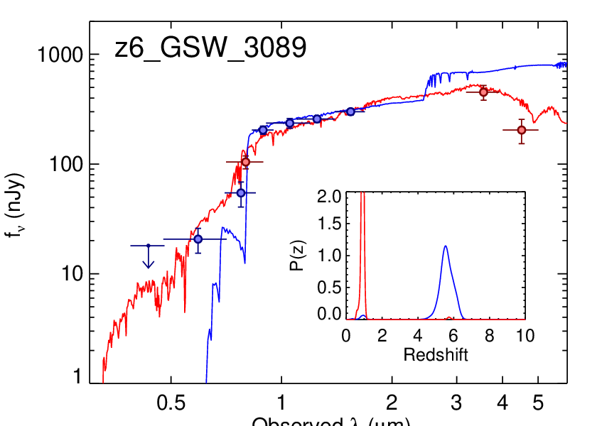
Examining these results, out of the 28 4 or 5 galaxies with preferred low-redshift solutions, 23 had photometry consistent with a true low-redshift galaxy. Four galaxies, however, had photometry which appeared to be consistent with a high redshift galaxy with a strong emission line (H or [O iii]) in one IRAC band. Systems with lines such as these (i.e., EW[OIII] 500 Å) are rare locally, but appear to be more common at high-redshift [154, 61, 141, e.g.,]. Although typical emission lines strengths are now included in the EAZY templates, these do not account for extreme emission lines, thus it is not surprising that EAZY does not return a high-redshift solution. We elect to keep these four galaxies in our sample, noting that the lack of strong rest-frame optical lines in the EAZY templates does not affect our initial sample selection, which does not make use of the IRAC photometry. A fifth galaxy (z5_GNW_13415) has a high-quality published spectroscopic redshift of 5.45, thus we also keep it in our sample. Perhaps unsurprisingly, the low-redshift fit for this galaxy had a very poor quality-of-fit, with 127, implying that the EAZY templates are a poor match for this galaxy. The remaining 23 galaxies at 4 and 5 were removed from our sample. The sole 6 galaxy with a preferred low-redshift solution with the inclusion of IRAC photometry, z6_GSW_3089, is shown in Figure 4. The red HST colors imply a much brighter IRAC flux than is seen. A solution at 0.93 yields a better fit, as the peak of stellar emission at that redshift better matches the observed IRAC fluxes. We have thus removed this galaxy from our sample. This galaxy has a spectroscopic redshift of 5.59 from the observations of Vanzella et al. [157]. However, this object has a spectroscopic quality flag of “C”, which indicates that the spectroscopic redshift is unreliable. This combined with the 4 detection in the band leaves us confident that a low redshift solution is more likely.
| Redshift | Nall | NM<-21 | Veff (M22) | Veff (M19) |
|---|---|---|---|---|
| (105 Mpc3) | (105 Mpc3) | |||
| 4 (3.5 – 4.5) | 4156 | 150 | 12.2 | 4.11 |
| 5 (4.5 – 5.5) | 2204 | 77 | 8.98 | 3.36 |
| 6 (5.5 – 6.5) | 706 | 28 | 7.93 | 2.50 |
| 7 (6.5 – 7.5) | 300 | 18 | 6.99 | 0.30 |
| 8 (7.5 – 8.5) | 80 | 3 | 5.88 | 0.16 |
Note. — The total number of sources in our final galaxy sample, after all contaminants were removed. The final two columns give the total effective volume at each redshift for two different values of the UV absolute magnitude.
With the removal of these likely contaminants, we retain a total sample of 150, 77, 28, 18 and 3 21 galaxies at 4, 5, 6, 7 and 8, respectively. The fraction of contaminants at 6 (one out of 50 6, 7, and 8 galaxies, or 2%) is consistent with (albeit somewhat less than) the expected low value calculated in §3.8 below.
Our final galaxy sample is summarized in Table 2, and a catalog of all galaxies in our sample is provided in Table 3. In Figure 1 we show the absolute UV magnitude distribution of our final samples, highlighting that we cover a dynamic range of five magnitudes. In particular, the CANDELS data are crucial, as galaxies from these data dominate the total number of galaxies in our sample, and approximately double the luminosity dynamic range which we can probe. This is highlighted in the left panel of Figure 2, which shows that galaxies discovered in the CANDELS GOODS fields dominate the total number at all redshifts in our sample.
| Catalog ID | IAU Designation | RA | Dec | M1500 | |
|---|---|---|---|---|---|
| (J2000) | (J2000) | (AB mag) | |||
| z4_GSD_27037 | HRG14 J033240.8275003.1 | 53.169922 | 27.834183 | 3.54 (3.45 to 3.63) | 20.45 (20.57 to 20.42) |
| z4_ERS_3675 | HRG14 J033235.0274117.5 | 53.145882 | 27.688189 | 4.08 (3.79 to 4.28) | 20.39 (20.47 to 20.15) |
| z4_GND_29830 | HRG14 J123718.1+621309.7 | 189.325211 | 62.219368 | 4.01 (3.85 to 4.17) | 19.68 (19.81 to 19.54) |
| z4_GND_30689 | HRG14 J123721.4+621259.2 | 189.339355 | 62.216450 | 3.66 (3.59 to 3.75) | 21.09 (21.16 to 21.03) |
| z5_GSD_8969 | HRG14 J033216.2274641.6 | 53.067379 | 27.778219 | 5.00 (4.87 to 5.14) | 20.62 (20.68 to 20.51) |
| z5_GND_31173 | HRG14 J123731.0+621254.2 | 189.379272 | 62.215046 | 4.85 (4.37 to 5.09) | 19.59 (19.77 to 19.43) |
| z5_MAIN_3271 | HRG14 J033243.5274711.4 | 53.181351 | 27.786510 | 5.50 (4.58 to 5.67) | 16.95 (17.05 to 16.78) |
| z5_PAR2_3762 | HRG14 J033304.8275234.7 | 53.270004 | 27.876295 | 4.47 (3.71 to 4.70) | 18.83 (18.97 to 18.57) |
| z6_GND_16819 | HRG14 J123718.8+621522.7 | 189.328232 | 62.256317 | 5.55 (5.41 to 5.65) | 21.56 (21.62 to 21.47) |
| z6_GNW_16070 | HRG14 J123549.0+621224.8 | 188.954025 | 62.206898 | 5.88 (5.64 to 6.02) | 20.83 (20.88 to 20.64) |
| z6_MAIN_2916 | HRG14 J033244.8274656.8 | 53.186806 | 27.782433 | 6.42 (5.79 to 6.76) | 18.39 (18.55 to 18.19) |
| z6_MACS0416PAR_145 | HRG14 J041632.2240533.3 | 64.134117 | 24.092587 | 5.91 (5.08 to 6.23) | 18.49 (18.64 to 18.16) |
| z7_GSD_12285 | HRG14 J033206.7274715.8 | 53.028114 | 27.787714 | 7.30 (6.44 to 7.89) | 19.57 (19.79 to 19.31) |
| z7_ERS_6730 | HRG14 J033216.0274159.2 | 53.066677 | 27.699766 | 6.74 (5.64 to 6.87) | 20.31 (20.31 to 19.96) |
| z7_GND_16759 | HRG14 J123619.2+621523.2 | 189.079834 | 62.256454 | 6.69 (6.33 to 6.89) | 20.89 (20.98 to 20.76) |
| z7_A2744PAR_4276 | HRG14 J001357.5302358.3 | 3.489512 | 30.399530 | 6.51 (6.26 to 6.78) | 19.37 (19.47 to 19.22) |
| z8_GSD_16150 | HRG14 J033213.9274757.7 | 53.057983 | 27.799349 | 7.91 (6.21 to 8.54) | 20.14 (20.38 to 19.91) |
| z8_MAIN_5173 | HRG14 J033241.5274751.0 | 53.172874 | 27.797487 | 8.11 (6.29 to 8.64) | 17.67 (17.98 to 17.41) |
| z8_GND_32082 | HRG14 J123727.4+621244.4 | 189.364258 | 62.212334 | 7.64 (7.02 to 8.16) | 20.27 (20.33 to 20.02) |
| z8_GND_8052 | HRG14 J123704.8+621718.8 | 189.270020 | 62.288559 | 8.10 (7.04 to 8.41) | 20.68 (20.84 to 20.44) |
Note. — A catalog of our 7446 4–8 galaxy candidates, with their derived properties. We include the IAU designation for continuity with previous and future works, with a designation prefix HRG14 denoting “High Redshift Galaxy 2014”. The values in parentheses represent the 68% confidence range on the derived parameters. Here, we show 20 representative galaxies, four from each redshift bin. This table is available in its entirety in a machine-readable form in the online journal. A portion is shown here for guidance regarding its form and content.
III.7. Stellar Population Modeling
To derive the rest-frame absolute magnitude at 1500 Å (), as well as the UV spectral slope [35, f], we fit spectral energy distributions (SEDs) from synthetic stellar population models to the observed HST photometry of our high-redshift candidate galaxies. The technique used here is similar to our previous works [57, 60, 59, 61]. We used the updated (2007) stellar population synthesis models of Bruzual & Charlot [31] to generate a grid of spectra, varying the stellar population metallicity, age, and star-formation history44 4 These models may overestimate the contribution of thermally pulsating asymptotic giant branch (TP-AGB) stars. However, these stars typically begin to dominate the emission at population ages 1 Gyr. Additionally, though the TP-AGB contribution may impact the SED in post-starburst galaxies at wavelengths as low as 0.5 m [83], our longest wavelength filter (1.6 m) at our lowest redshift ( 4) probes only 0.3 m, and all other filter/redshift combinations probe bluer rest-frame wavelengths. Thus, our choice to use the updated models should have no effect on our results.. Metallicities spanned 0.02 – 1 Solar, and ages spanned 1 Myr to the age of the Universe at a given redshift. We allowed several different types of star-formation histories (SFHs), including a single burst, continuous, as well as both exponentially decaying and rising (so-called “tau” and “inverted-tau” models). To these spectra, we added dust attenuation using the starburst attenuation curve of Calzetti et al. [34], with a range of 0 E(B-V) 0.8 (0 AV 3.2 mag). We also included nebular emission lines using the prescription of Salmon et al. [130], which uses the line ratios from Inoue [75], based on the number of ionizing photons from a given model, and assuming the ionizing photon escape fraction is zero. We then redshifted these models to 0 11 and added intergalactic medium (IGM) attenuation [92]. These model spectra were integrated through our HST filter bandpasses to derive synthetic photometry for comparison with our observations. For each model, we computed the value of by fitting a 100 Å-wide synthetic top-hat filter to the spectrum centered at rest-frame 1500 Å. Likewise, for each model we measured the value of by fitting a power law to each model spectrum using the wavelength windows specified by Calzetti et al. [35], similar to Finkelstein et al. [60].
The best-fit model was found via minimization, including an extra systematic error term of 5% of the object flux for each band to account for such items as residual uncertainties in the zeropoint correction and PSF-matching process. The stellar mass was computed as the normalization between the best-fit model (which was normalized to 1 M⊙) and the observed fluxes, weighted by the signal-to-noise in each band. These best-fit values of are used in our luminosity function analysis below, while is used to correct for incompleteness in a color-dependent fashion. The uncertainties in the best-fit parameters were derived via Monte Carlo simulations, perturbing the observed flux of each object by a number drawn from a Gaussian distribution with a standard deviation equal to the flux uncertainty in a given filter. For each galaxy, 103 Monte Carlo simulations were run, providing a distribution of 103 values for each physical parameter. The 68% confidence range for each parameter was calculated as the range of the central 68% of results from these simulations. In these simulations, the best-fit redshift was allowed to vary following the redshift probability distribution function, thus folding in the uncertainty in redshift into the uncertainty in the physical parameters [59, most notably, the stellar mass and ;]. During this process, we only allowed the redshift to vary within 1 of the best-fit photometric redshift. This excludes any low-redshift solution from biasing the uncertainties on a given parameter. The amount of the integrated at 3 excluded via this step was typically 10% (at 6).

III.8. Contamination
A key issue in any study of high redshift galaxies is the risk of sample contamination, either by spurious sources or by lower-redshift interlopers. The gold standard for eliminating contamination is to obtain spectroscopic redshifts. This is clearly unfeasible for all galaxies in our sample (until the next generation of space and ground-based telescopes), but there is significant archival spectroscopic data. As discussed in §3.2, we find excellent agreement between available spectroscopic redshifts and our photometric redshifts, with 0.031. In particular, the four bright55 5 Object z7_MAIN_2771 has a tentative spectroscopic redshift of 7.62, based on a 4 possible Ly emission line from Schenker et al. [134]. This object is quite faint, with , resulting in a somewhat large 95% photometric redshift confidence range of 6.02–7.74, though consistent with the tentative spectroscopic redshift. galaxies (24.9 25.7) with confirmed 6.5 have an excellent agreement with spectroscopic redshifts: z7_GNW_24443 with 6.66 and 6.573 [126], z7_GSD_21172 with 6.73 and 6.70 [71], z7_GNW_4703 with 7.19 and 7.213 [115], and z7_GND_42912 66 6 This source was originally called z8_GND_5296 in our previous catalog (Finkelstein et al. 2013). Our new catalog uses an updated version of the CANDELS GOODS-N data, thus the catalog numbering is different. Additionally, the slightly updated photometry pushes the photometric redshift of this galaxy slightly below 7.5, placing it in the 7 sample. with 7.45 and 7.51 [61]. The brightest source in our 6 sample, z6_GSW_12831 with 22.1 and z 5.77, is confirmed with 5.79 [32]. This galaxy has a 3 detection in the -band, which could have resulted in its exclusion from a typical LBG color-color selection sample [20, e.g.,], though the observed flux can be explained by non-ionizing UV photons transmitted through the Ly forest.
In general, spectroscopic followup of sources selected on the basis of their Lyman breaks (either color-color selection, or photometric redshift selection) finds a very small contamination by low-redshift sources [121, e.g.,]. However, given the apparent difficulty in detecting Ly emission at 6.5 [121, 115, 61, e.g.,], the true effect of contamination at these higher redshifts is not empirically known. In this subsection, we will attempt to estimate our contamination fraction by other means.
III.8.1 Properties of the Image Noise
Two key components of our selection processes should eliminate contamination by spurious sources in our sample. First, we restricted our sample to galaxies detected at 3.5 in two imaging bands: and . Formally, requiring a 3.5 detection in a single band should yield only a 0.05% contamination by noise. However, the wings of the noise distribution are highly non-Gaussian. We examined this by measuring the fluxes at 2105 random positions in the and images in the GOODS-S Deep field (see Schmidt et al. [138] for a similar analysis). To avoid biasing from real objects in the image, we only considered negative fluctuations [48, e.g.,], where the contamination percentage was computed as the ratio of the number of apertures with a flux 13.5 to the total number of apertures with negative fluxes. We found that in each of these bands individually, the fraction of positions measuring at 3.5 was 1.4%, much higher than predicted based on an assumption of Gaussian noise. If we instead look at the number of 3.5 fluctuations in both the and images at the same location, we find that this contamination drops to nearly zero, at 0.05%. Thus, we conclude that as we require significant detections in two bands, the contamination in our sample by noise is negligible. Spurious sources other than noise spikes are eliminated by our detailed visual inspection of each source, described in §3.3.
III.8.2 Estimates from Stacked Redshift PDFs
Contamination by low-redshift interlopers is a more complicated issue. While extreme emission line galaxies at lower-redshift could theoretically be an issue [7], our requirement of detections in two bands (as well as the frequent detections in more than two bands for all but the highest redshift objects in the 8 sample) makes a significant contamination by these sources unlikely. The most likely possible contaminants are faint red galaxies at 2 [47, e.g.,]. These galaxies can be too faint to be detected in our optical imaging, but their red SEDs yield detections in the WFC3/IR bands. Although faint sources that are very red will have a disfavored high-redshift solution with our current photometric selection, we have information on their likelihoods encoded in our redshift PDFs. Figure 5 shows the redshift PDFs of galaxies in each of our three highest redshift samples, stacked in magnitude bins of M 1 mag. At all redshifts and all magnitudes, 85% of the redshift PDF is at 4, implying that there is not significant contamination by lower-redshift galaxies.
The position of the secondary redshift peak is consistent with the detection of a 4000 Å break rather than the Lyman break (at 6, 7 and 8, this gives 1.1, 1,4 and 1.7). At 8, the possible contamination from galaxies at 4 is 10.5%, primarily due to the fact that at 8, a galaxy will have to be undetected in most of the filters we consider here (there is an additional 8% chance the true redshift is in the range ). The worst case is for faint galaxies at 6, as 6 galaxies are typically detected in all but two filters, though even here, the indicated contamination by 4 galaxies is 15%.
III.8.3 Stacking Imaging
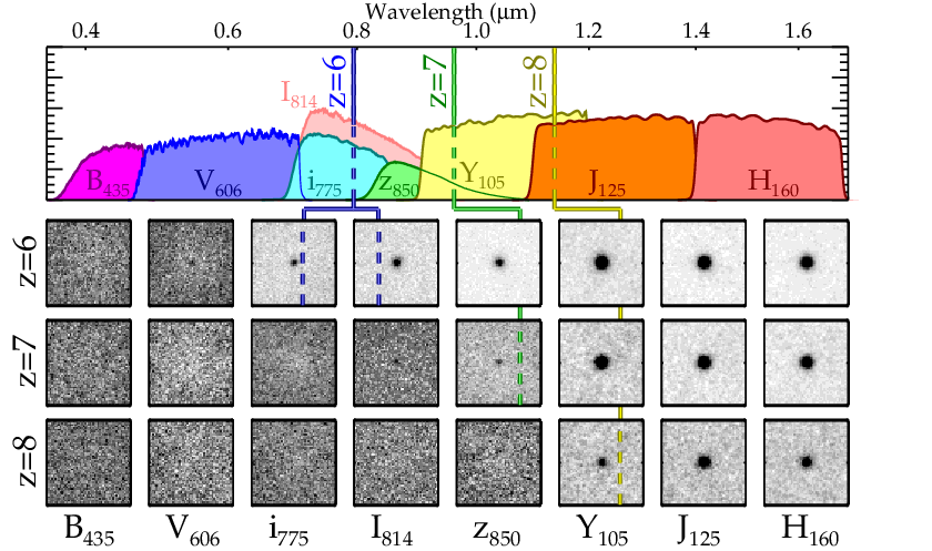
The limits from the previous subsection are likely upper limits on the contamination fraction. When fitting photometric redshifts, to rule out all low-redshift solutions, the Lyman break needs to be detected at high significance, which is the case for only the brightest galaxies (e.g., at 6, the brightest bin has a contamination of 2%). Additionally, these results are dependent on the templates used, which by definition do not account for unknown galaxy populations. We therefore consider two empirical tests of contamination. The first is to stack all galaxies in a sample, in order to search for detections below the Lyman break. The results from this test for 6, 7 and 8 are shown in Figure 6. As expected for galaxies at the expected redshifts, there is no visible signal in the -band at 6, -band and blueward at 7, and -band and blueward at 8. This confirms that the majority of the flux in our sample does not arise from lower-redshift sources.
III.8.4 Estimates from Dimmed Real Sources
As a final test, we estimated the contamination by artificially dimming real lower redshift sources in our catalog, to see if the increased photometric scatter allows them to be selected as high redshift candidates. This empirical test is useful as it does not rely on known spectral templates to derive the contamination, though it does assume that the fainter objects which could potentially contaminate our sample have similar SEDs to the bright objects which we dim. We performed this exercise twice, once using the combined catalog of the GOODS-S and GOODS-N Deep fields, and once in the HUDF main field, to probe fainter magnitudes. In the GOODS Deep fields, we selected all real sources with 21 24 and , and reduced their observed fluxes by a factor of 20. The same was done for sources drawn from the HUDF Main field, here extending the magnitude range to be 21 26. The limits on these magnitudes were chosen to exclude any real high-redshift sources. We replaced the true flux uncertainties of these objects with flux uncertainties from a randomly drawn real source from the full catalog from a given field with a similar magnitude as the dimmed source. We then added scatter to the dimmed fluxes, perturbing them by a random amount drawn from a Gaussian distribution with a standard deviation equal to the flux uncertainties of the object. We included two realizations of the HUDF field to increase the number of dimmed objects.
The total number of sources in our artificially dimmed catalog was 4066 in the Deep fields, and 1254 in the HUDF field. We measured photometric redshifts of these sources with EAZY in an identical manner as on our real catalogs, and then we applied our sample selection to this dimmed catalog. In the Deep fields, we found a total number of 149, 134, 54, 23 and 8 dimmed objects satisfied our 4, 5, 6, 7 and 8 selection criteria. Investigating the original (not dimmed or perturbed) colors of these sources, we found that they are unsurprisingly red, with the bulk of sources having 2 mag. It is therefore this parent population of red sources which are responsible for the majority of the possible contamination. The contamination fraction in our high-redshift sample is then defined as
| (1) |
where was the number of dimmed sources satisfying our high-redshift sample selection, was the total number of sources in the dimmed catalog with original colors of 2, was the number of sources in the full object catalog with 25 27, 3, and 2, and was the number of true galaxy candidates in a given redshift bin. For example, at 6, where we found 54 dimmed galaxies satisfied our selection criteria ( =54), 1023, 695, and 322, giving an estimated contamination fraction 11.4%. Thus for sources with 25 27, we found an estimated contamination fraction of 4.5%, 8.1%, 11.4%, 11.1% and 16.0% at 4, 5, 6, 7 and 8, respectively. We performed the same exercise in the HUDF, here for fainter sources with 26 29, finding 30, 21, 8, 8 and 0 sources satisfied our 4, 5, 6, 7 and 8 selection criteria, giving a contamination fraction of 9.1%, 11.6%, 6.2%, 14.7% and 4.9% at 4, 5, 6, 7 and 8.


Broadly speaking, we estimate relatively small contamination fractions of 5-15%, in line with the estimates above from the stacked curves. As the bulk of contaminants appear to be red galaxies, it is interesting to compare to the space density of these potentially contaminating sources. This was recently estimated by Casey et al. [38], who find that dusty star-forming galaxies at 5 will contaminate 5 galaxies samples at a rate of 1%. This is much less than our contamination estimates, thus we may have overestimated the contamination rate, though it may not be inconsistent once photometric scatter is applied to faint, red galaxies, making it easier for them to scatter into our sample. In any case, the expected contamination rate is quite small, therefore we do not reduce our observed number densities for the expected minimal contamination.
IV. Completeness Simulations
We performed an extensive set of simulations to estimate the effective volume for each source in our sample, accounting for both image incompleteness and selection effects. We inserted mock galaxies into the imaging data, repeating the same analysis for source detection, photometry, photometric redshift measurement, and sample selection as was done on the real data. We then compared the fraction of recovered and selected mock sources to the total number of input sources in a given bin of absolute magnitude and redshift to determine our completeness in that bin.
While the effective volumes are typically computed as a function of magnitude and redshift, other key factors in these simulations are the choices of galaxy size and color. At a constant magnitude, a very extended galaxy may not make it into our sample, as it may fall below our surface brightness sensitivity. Additionally, very red galaxies may not satisfy our selection criteria, as red colors typically enhance the amplitude of the low-redshift solutions, particularly at low signal-to-noise levels. Thus the effective volume depends not only on magnitude and redshift, but also on the size and rest-frame UV color. To see what effect this has, we have computed our completeness as a function of four properties: redshift, absolute magnitude, half-light radius, rest-UV color, where we have parametrized the latter via the UV spectral slope [35]. A large number of simulated objects are needed to fill out this four-dimensional space; our completed simulations recovered 5.4 million out of 7 million objects input across all of our fields (where the recovered objects were detected in our photometry catalogs; this number does not account for the photometric redshift selection, which we discuss below).
Our simulations were run separately on each of our 10 sub-fields defined in Table 1. To ensure that the mock galaxies did not affect the background estimation, only a small number of galaxies were added during each simulation. To optimize the simulation runtime, the mock galaxies were added to cutouts from the full images. In the GOODS sub-fields (i.e., CANDELS Deep and Wide, and the ERS), 200 mock galaxies were added to a 20002000 pixel (2) region of the images, while for the single-pointing HUDF and HFF fields, 100 galaxies were added to a 10001000 pixel region. As the depth across our imaging data can vary, during each simulation the position of the cutout varied, such that when we combine all of our simulations, we average over any differences in the depth across a given field.
To determine the colors of the mock galaxies, we created distributions in redshift, dust attenuation (parameterized by E[B-V]), stellar population age and stellar metallicity. The redshift distribution was defined to be flat across 3 9, such that we simulate objects well above and below the redshift ranges of interest. The dust attenuation E(B-V) was defined to have a Gaussian distribution with a mean of 0.1 and a 0.15 (with a minimum of zero). The age was defined as a log-normal distribution, with a peak near 10 Myr, and a tail extending out to the age of the Universe at a given redshift. The metallicity distribution was also log-normal, with a peak of ⊙, and a tail towards higher values. The exact values of these distributions are not crucial given our methodology (as opposed to a multivariate analysis, where the distributions are very important), as they combine to create a distribution of rest-frame UV slope . We crafted these distributions to provide a distribution of encompassing the expected values for our real objects [60, 26, e.g.,]. We then used the updated (2007) stellar population models of Bruzual & Charlot [31] to calculate the colors of a stellar population given the distributions above. To convert these colors into magnitudes, we assumed a distribution of -band magnitudes designed to have many faint ( 26) galaxies (which is where we expect to become incomplete), and relatively few at bright magnitudes. To ensure enough bright galaxies to calculate a robust incompleteness, every 10th simulation used a flat distribution of -band magnitudes of 22 25. These -band magnitudes were combined with the mock galaxy colors to generate magnitudes in each filter for a given field.
To generate the galaxy images themselves, we used the GALFIT software [120]. We assumed a log-normal distribution of half-light radii with a peak at 1-pixel, and a high tail towards larger radii, giving an interquartile range of half-light radii of 1.4–4.9 pixels. This corresponds to 0.4–1.6 kpc, spanning the range of the majority of resolved galaxies at 4 [109, 68, 116, 44, e.g.,]. GALFIT also requires a Sersic index (), axis ratio and position angle; the Sersic index was assumed to be a log-normal distribution at 1 4, with the majority of the mock galaxies having disk-like morphologies ( 2); the axial ratio was also log-normal, with a peak at 0.8, and a tail toward lower values, and the position angle was a uniformly distributed random value between 0 and 360 degrees. GALFIT was then used to generate a 101101 pixel (6) stamp for a given mock galaxy, which was then added to the image at a random location. Because our data are PSF-matched to the -band, we had GALFIT convolve the mock galaxy images with the -band PSF prior to adding them to the data for all filters.
Once the set of mock galaxies for a given simulation were added to the data, photometric catalogs were generated using Source Extractor in the exact same manner as was done on the data (i.e., using a weighted image as the detection image). These catalogs were read in and combined, again in the same methodology as with the data, including aperture corrections (the exception here is that a correction for Galactic extinction was not applied in the simulation, as the simulated objects did not have Galactic extinction included). The photometric catalog was then compared to the input catalog to generate the list of recovered objects (i.e., mock galaxies which were recovered by Source Extractor); an object was regarded as being recovered if it had a positional match within 0.2′′ of one of the input mock galaxies. The recovered object catalogs were processed through EAZY to generate photometric redshifts, and then run through our SED-fitting routine to measure absolute UV magnitudes (), stellar masses and UV spectral slopes. These simulations were then repeated until a large sample of recovered galaxies was available, which were then compiled in a single database per field. The completeness was defined as the number of galaxies recovered versus the number of input galaxies, as a function of input absolute magnitude, redshift, half-light radius and UV spectral slope . Figure 7 shows the results from our simulations.


In our original simulations the recovered redshift was typically 0.2 lower than the input redshift, independent of magnitude. This is likely not a fault in our photometric redshift estimates, as Figure 2 shows that these agree well with existing spectroscopic redshifts for real galaxies. Rather, it is likely a mismatch between our simulated SEDs and those of the templates used in EAZY. Upon further investigation, we found that the cause of this offset was Ly emission in the mock galaxies. While Ly photons were attenuated by dust in the same manner as adjacent UV photons, we did not include any additional Ly attenuation for, e.g., geometric or kinematic effects. This led to very high Ly escape fractions, which were not matched in the templates. This high Ly emission reduced the amplitude of the photometrically-measured Lyman break, resulting in a (slightly) lower photometric redshift. After reducing the amount of Ly flux to 25% of the intrinsic value, our photometric redshifts matched the input redshifts (which matches expectations for the global Ly escape fraction; Hayes et al. [73, e.g.,], Blanc et al. [16, e.g.,]. Rather than rerun all of our completeness simulations, we elected to simply reduce the input redshift by 0.2 when interpreting our simulations, which corrects for this effect (this changes the distance modulus by 0.1 mag). The exception was the simulations for the HFF parallel fields, which were run after this effect was noticed. In those fields, the input models had their Ly flux reduced to 25% of the intrinsic value, and no change to the model redshift was needed.
It is important to examine whether the choice of computing the completeness as a function of input properties affects our result. As mentioned in §2.3, we used the results from these simulations to correct for offsets in the recovered versus input magnitudes (i.e., to be sure the fluxes we use represent the total flux). Additionally, we examined whether there exist biases in the half-light radius or measurements from the simulations. Recovered objects were typically measured to have a half-light radius 0.03′′ (0.5 pixels) smaller than the input value, and were measured to be slightly redder ( 0.1). However, these corrections make effectively no change to the effective volumes derived from the simulations, and so were not applied.
In each redshift bin, the effective volume for galaxies in a given field was then calculated via
| (2) |
where is the comoving volume element, and is the result from our completeness simulations. The integral was done over 1, centered on the center of each redshift bin. In each field, we used a weighted mean of this three-dimensional effective volume to calculate , where the weighting is based on the number of real objects in a magnitude bin with a given value of rh and , as
| (3) |
This assumes that the completeness corrections estimated using our observed size and color distributions are similar to what we obtained if we could measure the true sizes and colors, motivated by our measurement of minimal size and color biases when comparing the input to recovered values.
This weighted volume is the most representative of the true volume we are sensitive to, as we explicitly account for the incompleteness as a function of size and color. Figure 9 highlights the dependence of the effective volume on these quantities for galaxies in our 6 sample in the GOODS-N Deep field. The effective volume has a strong dependence on the surface brightness of galaxies, as the volume drops steeply both for larger sizes and fainter magnitudes. The central and right panels highlight that while the effective volume (and thus sample completeness) is sensitive to both size and color, the color has a relatively minor role. We remain sensitive to fairly red galaxies (1), similar to previous results from Bouwens et al. [25]. Although the effective volume has a strong dependence on size, the relatively small sizes of galaxies in our sample yields a volume similar to that obtained when assuming a constant small size. Thus, although our volumes are the most accurate, had we assumed a fixed effective radius of, e.g., r 1 kpc, our results would not change significantly. This is consistent with the conclusions of Grazian et al. [68] who found, accounting for the size-luminosity relation when deriving the 7 luminosity function, similar results as previous studies that neglected the size-luminosity relation. Our final effective volumes are shown in Figure 8.
V. The Luminosity Function
V.1. Parametric Approach
Possessing our final galaxy sample with measured values of , as well as the effective volumes from our completeness simulations in the previous section, we can now proceed to measure the rest-frame UV luminosity function at 4, 5, 6, 7 and 8. We calculate the luminosity function in two ways: a parametric version assuming that the luminosity function takes the form of a Schechter [133] function, and a non-parametric step-wise maximum likelihood (SWML) calculation.
The fitting of a Schechter function is well motivated, as it successfully matches the observed rest-UV luminosity functions at lower redshifts [124, 19, e.g.,]. This function is characterized by a power-law at the faint end with slope , and an exponential cut-off at the bright end, transitioning between the two regimes at the characteristic magnitude M∗. The parameter sets the normalization of this function. The number density at a given magnitude is then given by
| (4) |
For the measurement of the luminosity function assuming a Schechter functional form, we calculated the likelihood that the number of observed galaxies in a given magnitude bin is equal to that for an assumed value of the Schechter parameters and . Rather than performing a grid-based search, we performed a Markov Chain Monte Carlo (MCMC) search algorithm, to better span the parameter space, as well as to better characterize the uncertainties on the Schechter parameters. We performed this calculation in bins of absolute magnitude with M 0.5 mag, ranging from 24 17. At the bright end we are in the limit of small numbers, therefore we model the probability distribution as a Poissonian distribution [39, 129, e.g.,], with:
| (5) |
| (6) |
where is the likelihood that the expected number of galaxies () matches that observed () for a given value of and , and is the goodness-of-fit statistic. The subscripts and represent the sub-fields and magnitude bins, respectively. The final goodness-of-fit is the sum over all fields and magnitudes in a given redshift bin. We use the effective volume results for a given redshift, magnitude bin, and field to convert from the model number density to the expected number, calculating as the normalization such that the total expected number of galaxies over all magnitude bins matches the total number of observed galaxies.


For each magnitude bin, we performed 10 independent MCMC chains utilizing a Metropolis-Hastings algorithm, each of 105 steps, building a distribution of , and values for each field. During each step of the chain, the likelihood of a given model was computed for each of our observed fields, and then added together to compute the likelihood for the sample as a whole (we also recorded the individual field values, see §6.5). Prior to each recorded chain, we performed a burn-in run with a number of steps equal to 10% of the number of steps in each chain. The starting point for the burn is a brute-force fit of a grid of and values to our data. At the end of the burn, the final values of the parameters from the last step were then the starting points for each chain. The burn-in results were not otherwise recorded. During each step, new values of and were chosen from a random Gaussian distribution, with the Gaussian width tuned to generate an approximate acceptance rate of 23%. During each step was calculated as the normalization. If the difference between the likelihood of the model for the current step exceeds that from the previous step by more than a randomly drawn value ( 2 ln (); where is a uniform random number between zero and unity), then the current values of the Schechter function parameters were recorded. If not, the chain reverted to the value from the previous step.
By running 10 independent chains, we mitigate against being trapped by local minima in the parameter space. Our final result concatenates these 10 chains together, giving a distribution of 106 values of the Schechter function parameters at each redshift. The results were visually inspected to confirm that the chains reached convergence. For each Schechter function parameter, the best-fit values were taken to be the median of the distribution, with the uncertainty being the central 68% of the distribution. These results are given in Table 4. For the 8 Schechter function fit, we imposed a top-hat prior forcing to be fainter than 23. Without this prior, the fit preferred a much brighter value of , such that the observed data points all lay on the faint-end slope (i.e., a single power law). We discuss the implications of this in §6.6.
Although we computed the volumes down to very faint magnitudes, should we include these faint galaxies and calculate the luminosity function down to 17 or fainter, we would be highly incomplete (Figure 8). In practice, it is our deepest field (the HUDF) which determines how faint we can constrain the luminosity function. The HUDF drops below 50% completeness at magnitudes fainter than 17.5 at 4, 5 and 6, 18 at 7, and 18.5 at 8. Thus, in our calculation of the luminosity function, we only include a given field’s contribution at a given magnitude if it is above the 50% completeness limit for that magnitude and redshift. Extending the analysis fainter will give results dominated by the incompleteness correction.
As shown in Figure 8, while the volume per unit area for the different fields is very tight at 4, there is a progressively larger scatter apparent when moving towards higher redshift, representing a systematic uncertainty in the effective volume calculation. One likely culprit is the fact that the volumes depend on the distribution of the sizes and colors of objects in a given field. For fields with few sources (i.e., the smallest fields at the highest redshifts), there may be only a single object in a given magnitude bin. To mitigate significant variances in the effective volume at the bright end, where numbers of sources are small, we set the effective volume in a given redshift bin and field in bright bins with less than three objects equal to the value in the brightest bin with more than three objects (i.e., if there are no magnitude bins with more than three objects at M 21, the effective volumes for all brighter bins are set equal to the value at M 21). This change has no discernable effect on our luminosity function results as this is well above the 90% completeness limit for any of our fields, and is thus only done to keep small numbers of galaxies from significantly affecting the volumes.
| Redshift | M∗ | ||
|---|---|---|---|
| (Mpc-3) | |||
| 4 | 20.73 | 1.56 | (14.1) 10-4 |
| 5 | 20.81 | 1.67 | (8.95) 10-4 |
| 6 | 21.13 | 2.02 | (1.86) 10-4 |
| 7 | 21.03 | 2.03 | (1.57) 10-4 |
| 8 | 20.89 | 2.36 | (0.72) 10-4 |
Note. — The final values for each parameter are the median of the parameter distribution from the MCMC analysis. The quoted errors represent the 68% confidence range on each parameter.
| M1500 | 4) | 5) | 6) | 7) | 8) |
|---|---|---|---|---|---|
| (10-3 Mpc-3 mag-1) | (10-3 Mpc-3 mag-1) | (10-3 Mpc-3 mag-1) | (10-3 Mpc-3 mag-1) | (10-3 Mpc-3 mag-1) | |
| -23.0 | 0.0016 | 0.0023 | 0.0025 | 0.0029 | 0.0035 |
| -22.5 | 0.0093 | 0.0082 | 0.0025 | 0.0029 | 0.0035 |
| -22.0 | 0.0276 | 0.0082 | 0.0091 | 0.0046 | 0.0035 |
| -21.5 | 0.1192 | 0.0758 | 0.0338 | 0.0187 | 0.0079 |
| -21.0 | 0.2968 | 0.2564 | 0.0703 | 0.0690 | 0.0150 |
| -20.5 | 0.6491 | 0.5181 | 0.1910 | 0.1301 | 0.0615 |
| -20.0 | 1.2637 | 0.9315 | 0.3970 | 0.2742 | 0.1097 |
| -19.5 | 1.6645 | 1.2086 | 0.5858 | 0.3848 | 0.2174 |
| -19.0 | 2.6392 | 2.0874 | 0.8375 | 0.5699 | 0.6073 |
| -18.5 | 3.6169 | 3.6886 | 2.4450 | 2.5650 | 1.5110 |
| -18.0 | 5.8343 | 4.7361 | 3.6662 | 3.0780 | — |
| -17.5 | 6.4858 | 7.0842 | 5.9126 | — | — |
Note. — Magnitude bins with zero objects are shown as upper limits, calculated as 1/Veff/M in that magnitude bin for that redshift.
Another possible issue is the source density of simulated objects. In the smaller fields (HUDF, HUDF parallels, HFF parallels) we input sources with twice the surface density as in the larger fields to speed up the computing time. As some sources (just like real galaxies) will inevitably fall on top of real sources, and thus not be recovered, an increased source density could result in a (slightly) lower completeness. This is just what is observed in these fields, as shown in Figures 7 and 8. To account for this uncertainty, we measured the spread in volume per unit area in each field at 21 at each redshift, which we found to be 1.5%, 3.8%, 6.2%, 7.8% and 13% at 4, 5, 6, 7 and 8, respectively. At each step in the MCMC chain, we perturbed the effective volume by this amount to account for this systematic uncertainty in our luminosity function results.
V.2. Non-Parametric Approach
We have also examined a non-parametric approach to studying evolution in the luminosity function. This is particularly warranted at very high redshift, where the effects responsible for suppressing the bright end of the luminosity function and causing the exponential decline in number density (e.g., active galactic nuclei feedback, or dust attenuation) may be less relevant. We thus calculated the SWML luminosity function, which is essentially the number density at a given magnitude, free from assumptions about the functional form of number density with magnitude. We also calculated the SWML luminosity function using an MCMC sampler. In this case, as the number densities in the magnitude bins are not linked by an overarching function, we calculated the number density in each magnitude bin independently.
For each magnitude bin and for each field, the likelihood was calculated (using Equations 5 and 6 above) that a given randomly drawn value of will give the observed number of galaxies. The actual recorded value of is that which maximizes the likelihood. While in practice, this yields very similar results as one would get by simply taking the observed number and dividing by the effective volume (consistent within a few percent for bins with more than a few galaxies), our approach has two advantages. First, in the limits where numbers are small, this approach is more accurate in that it properly accounts for the Poissonian likelihood. Secondly, this approach generates a full probability distribution for the number densities in each magnitude bin, allowing for the derivation of accurate asymmetric uncertainties. Our SWML luminosity function determinations and best-fit Schechter functions are given in Table 5 and shown in Figure 10.
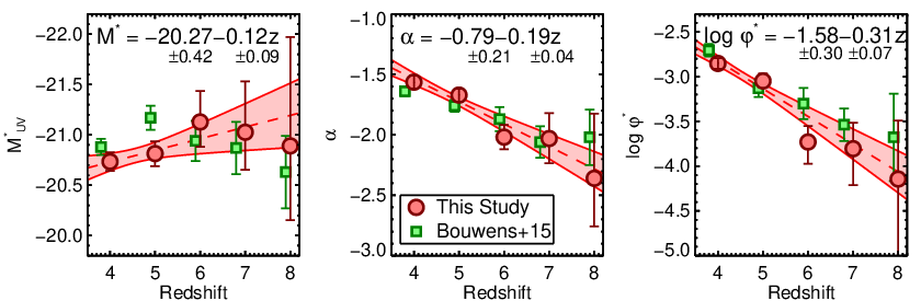
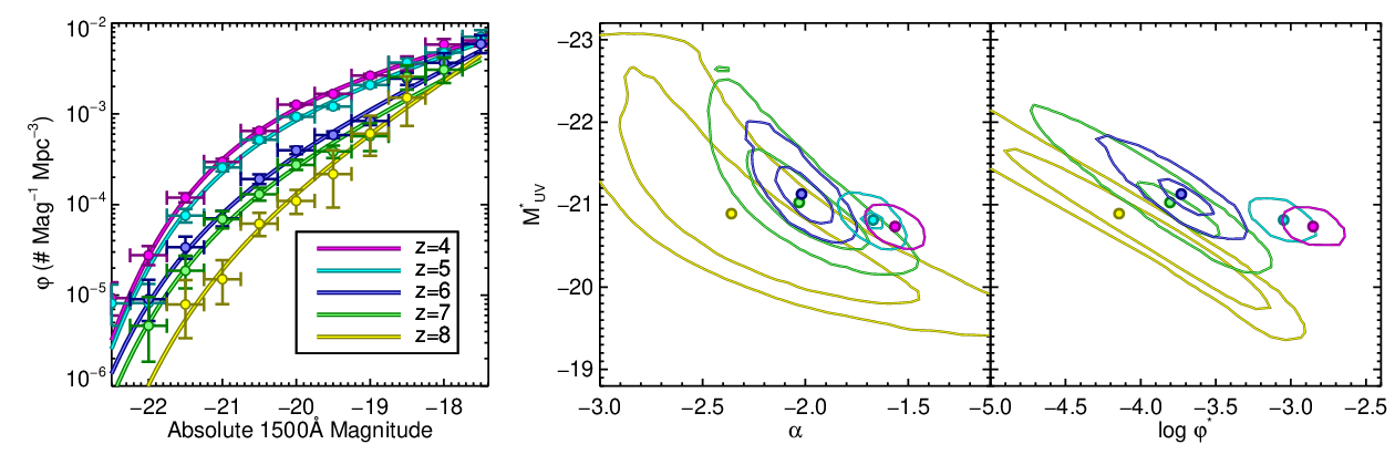

VI. Luminosity Function Interpretation
VI.1. Evolution
As shown in Figure 10, the qualitative shape of the SWML luminosity functions at all redshifts we consider here are similar, in that bright galaxies are rare and faint galaxies are relatively common. Additionally, when examining the Schechter fits (solid line), we see that they are consistent with the SWML determinations. The best-fit Schechter function parameters (Table 4) surprisingly show little evolution in . However, from 4 to 8, the uncertainty on gets progressively larger, to 0.4 (0.9) mag at 7 (8). This is easy to understand, as at all redshifts, our dataset contains galaxies in only 1-2 bins brightward of . Ideally, one would prefer to have multiple bins in magnitude on either side of to obtain robust constraints. As shown here, that will require a larger volume than we consider in this analysis. In Figure 11, we also fit the evolution of with redshift with a linear function, using our results at 4–8. We find that 0.12 0.09; thus, our data do not support a significant evolution of with redshift.
We also fit similar functions to see if we detect evolution in and . As shown in Figure 11, we do see significant evolution in the faint-end slope , with it becoming steeper at higher redshift, as 0.19 0.04 (4.8 significance). We see a similar significance in the evolution of the characteristic number density , which evolves as 0.31 0.07 (4.4 significance). Thus, while does not significantly evolve with redshift from 4 to 8, both and do, in that the number density decreases and the faint-end slope becomes steeper with increasing redshift. In particular, this decline in characteristic number density is by a factor of 20, over a period of time of less than 1 Gyr. Although the steepening of the faint end is consistent with previous studies [25, e.g.,], the un-evolving and strong number density evolution are the opposite of the picture presented in the literature just one year ago [20, 24, 99, e.g.,]. This updated evolutionary picture will be crucial when projecting number counts for future HST and James Webb Space Telescope surveys.
In Figure 12, we show our determinations of the luminosity functions together at all five redshifts, along with the joint confidence contours on , and . It is apparent that there is significant evolution in the luminosity function, with a drop in number density from 4 to 8, as well as a gradual steepening of the faint-end slope. The apparent non-evolution of the characteristic magnitude is visible as the roughly constant magnitude of the “knee” of the luminosity function.
VI.2. Impact of Magnitude Uncertainties
By definition, our method of computing the luminosity function is dependent on magnitude binning, as we compare the observed number to that expected based on a given model in magnitude bins of width 0.5 mag. While galaxies close to one side of a magnitude bin have the potential to scatter to another bin, the typical uncertainties on the UV absolute magnitudes of galaxies in our sample are 0.2 mag. Additionally, galaxies can shift both ways, thus while one galaxy moves out of a bin, another may move in, though this effect will not be symmetric given the shape of the luminosity function. In our results above, we had assumed that magnitude scatter does not significantly impact our results.

To investigate the impact of this assumption, we performed another iteration of MCMC fitting to our data, here allowing galaxies to scatter between magnitude bins. At each step in the MCMC chain, a new value of was drawn for each galaxy from the 100 SED-fitting Monte Carlo simulation results. The spread in these values encompassed both the photometric scatter in the observed filters and the uncertainty in the photometric redshift (see §3.7). To compare to our fiducial luminosity function values, we recorded both the median Schechter parameter results and the median number density in each magnitude bin, as, unlike our fiducial MCMC run, these varied during each step as the magnitudes changed. At all redshifts, our fiducial values of the step-wise luminosity functions are consistent with these “magnitude-scatter” values within 10% at M 21.5, and typically within 2-3%. The sole exception is in the brightest bin (22 at 4–6, and 21.5 at 7 and 8), where our fiducial number density values are higher by 15-20% (60% at 7, where there is only a single galaxy in this bin). We examined the Schechter fit, to see whether this bright-end difference affects our results. Values of both and derived when allowing galaxies to shift between bins are consistent with our fiducial values within 0.1 mag and 3%, respectively. We conclude that the relatively small (20%) uncertainties in the absolute magnitudes of our galaxies do not have a significant impact on our luminosity function results.
VI.3. Non-parametric Evolution
Given that our results show that the Schechter functional parameters may not be a robust method of tracking galaxy evolution (e.g., a non-evolving value of does not mean that the galaxy populations are not evolving), we examine the evolution in a non-parametric way. In Figure 13 we show the evolution of the step-wise luminosity function, plotting the number density corresponding to galaxies at M21 and 19 versus redshift. From 8 to 4 the abundance of brighter galaxies increases faster than faint galaxies. This trend halts at 4, where bright galaxies have an approximately constant abundance down to 2, and then turns over. Faint galaxies, however, continue increasing in abundance down to 2, where they also turn over. This figure highlights the phenomenon of downsizing, where bright/large galaxies grow faster at early times [e.g., 42, see also Lundgren et al. 2014]. This is different from the expectation one would get simply from examining Schechter fits, as the luminosity functions don’t evolve much over the range 2 4 [124, e.g.,]. Given that the trends here mimic the evolution of the cosmic SFR density, we fit the function provided by Madau & Dickinson [93] to our data for both number densities, given by
| (7) |
The evolution with redshift is thus proportional to ()α at low redshift, and ()α-γ at high redshift, with and as dimensionless coefficients. Fitting the data in this way, we confirm that at 3, bright galaxies change in abundance faster, as ()-5.9±0.4, than faint galaxies, which go as ()-3.3±0.3.
Another interesting aspect is to compare the trends observed to our predicted abundance of bright 9 galaxies (see §9). The trend observed here slightly overestimates our predicted 9 abundance, though if we assume the uncertainties on our 8 number density applies to 9, our trend is consistent with this prediction. In any case, this trend of abundance with redshift lends more weight to our expectation of a significant abundance of bright 9 galaxies. This figure neglects the impact of dust attenuation, as we are only looking at the observed UV magnitudes. The dust attenuation appears to be luminosity dependent (bright galaxies are dustier than faint galaxies, e.g., Bouwens et al. 2013), as well as being higher at lower redshift. Thus, correcting for dust would not only increase the abundance of bright galaxies more than that of faint galaxies, it would increase it by more at lower redshift, thus enhancing the differences between faint and bright galaxies at 4.
VI.4. Comparison to Previous Results
Our result of a similarly bright value of at 6, 7 and 8 is a dramatic change from previously published results. In Figure 10, we show the step-wise luminosity function results from several relevant studies from the literature. Figure 14 shows our uncertainty results, highlighting both the distribution of and from the MCMC chains, as well as the covariance between the two parameters, along with previous determinations of and [20, 97, 117, 153, 24, 99, 135, 161, 29]. In this subsection we compare solely to previous work - we reserve the comparison to the contemporaneous work by Bouwens et al. [27] to §6.4.1 below.
At 4 and 5, both our binned luminosity function data points as well as our Schechter function parameters are in excellent agreement with the ground-based study of van der Burg et al. [153]. We are also in excellent agreement with the ground-based study of McLure et al. [97] at 5. We find good agreement with the space-based study of Bouwens et al. [20] at 5, but at 4 the Bouwens et al. [20] result lies outside our 2 confidence region on the Schechter function parameters, in that we prefer a shallower faint-end slope and a fainter value for .
At 6, our binned luminosity function data points are consistent within 1-2 with the Bouwens et al. [20] results at the faint end (Figure 10). At the bright end, our data are higher than those from both ground-based studies (though again, typically only different at the 1-2 level). This is somewhat counter-intuitive, as one may expect the ground-based studies to suffer a higher contamination rate, particularly for relatively fainter sources at higher redshift, due to their inability to resolve stars from galaxies, but it may also be explained due to an aggressive sample selection required to minimize contamination. In any case, the differences are not highly significant, with the exception of the brightest data point from Willott et al. [161], which gives a number density at 22.5 of 2.7 10-8 Mpc-3. While this is consistent with our upper limit at that magnitude, it is a factor of 250 lower than our number density only 0.5 mag fainter at 22 (see Table 5). Given the results at similar magnitudes at lower redshifts, it is highly unlikely that there is such a steep drop in number density over only a 0.5 magnitude interval, though future large area studies can better investigate the difference (Bowler et al. in prep). The larger discrepancy comes when comparing the Schechter function parameters. Specifically, Bouwens et al. [20] found M20.29 0.19, and McLure et al. [97] found M20.04 0.12. Both values are significantly (2–3) fainter than our derivation of M21.13. For the space-based study of Bouwens et al. [20], this is understandable, as at that time only optical data were available, thus 6 galaxies were selected via detections in only one band, and a robust determination of their UV absolute magnitudes was difficult. For the ground-based study of McLure et al. [97], a cause for the difference is less clear, though certainly the different data being used plays a role.
Comparing to previous works at 7, we find broadly similar results, in that our results are consistent with the derived number densities from previous studies, yet our Schechter fit prefers a much brighter value of . This is easier to understand, as a number of previous studies had less data available, and thus, utilizing smaller volumes, were unable to constrain the bright end [24, 135, e.g.,]. The exception is the recent work by McLure et al. [99], which used a similar volume as our study, though they used the CANDELS UDS field in place of our use of the CANDELS GOODS-N field. Examining the brightest data point from McLure et al. [99] at 21, the number density is about a factor of two below our data point. However, the discrepancy is mitigated by two factors. First, as discussed by Bouwens et al. [27], the use of fixed diameter circular apertures by McLure et al. [99] systematically underestimates the fluxes for bright, more extended, galaxies. Bouwens et al. [27] estimated the amplitude of this effect to be 0.25 mag. Shifting the brightest McLure et al. [99] data point by 0.25 mag brings it into agreement with our results. Secondly, the CANDELS GOODS-N field appears to have an overdensity of 7 galaxies. Specifically, when comparing the number density of 7 galaxies in the GOODS-N Deep field to the GOODS-S Deep field in Figure 16, GOODS-N has a higher number density at all magnitudes. While we have not selected galaxy samples in the UDS, we can examine this further by recomputing our 7 stepwise luminosity function using only the GOODS-S and HUDF fields. At magnitudes fainter than 21 the results do not change appreciably, as the GOODS-N Deep and Wide fields lie on either side of our Schechter fit at those magnitudes. However, the results using only GOODS-S provide a number density 33% lower at 21.5 than our fiducial luminosity function. This difference is at the 1 level due to the large Poisson noise contribution in this bin, and thus is not highly significant.
We also compare to several ground-based studies at 7. Ouchi et al. [117] identified 22 bright 7 candidate galaxies over 0.4 deg2. Their data points based on detected galaxies are consistent with our own, though their strict upper limits at 22 push their Schechter fit to a fainter value of M20.1, although the large uncertainty (0.76) leaves consistent with our fit at only slightly more than the 1 level. The stepwise luminosity function from Castellano et al. [40] based on deep HAWK-I data agrees well with our results, while the results from the zFourGE medium band survey of Tilvi et al. [149] agree at M21.5, but differ by 2 at M 20.5.
Recently, Bowler et al. [29] have made a significant improvement in search volume from the ground, discovering 34 luminous 7 galaxy candidates over 1.65 deg2, from the UltraVISTA survey data over the COSMOS field [96] and the UKIDSS survey over the UDS field [87]. Broadly speaking, they are consistent with our results, and they are highly inconsistent with the previous determinations of M20 (Figure 10). There is a mild tension at 21.75, where the value of our Schechter fit at that point is 2 higher than their derived number density. However, this is their faintest magnitude bin, and is only 50% complete, thus this data point relies the most on the completeness correction. In any case, the fact that Bowler et al. [29] found 7 candidates out to very bright magnitudes gives us confidence that our brighter determination of is not necessarily dominated by cosmic variance in our fields, but is a true feature of the 7 universe. However, our present uncertainty on of 0.4 mag makes it apparent that more data are needed to constrain this parameter further.
At 8, we again find consistent number densities with previous studies, though our larger volume allows us to find more rare, bright (21.5) galaxies than observed in some previous surveys, pushing them to lower values of (though again here our uncertainty on is large, so the difference in our determination is not significantly different from previous studies). As noted above, in our fit of the 8 luminosity function, we constrained to be fainter than 23, to avoid un-physically bright values, which tended to be preferred in an unconstrained fit. We note two important points when comparing to previous studies. First, while our study did not utilize the pure parallel BoRG [152] and HIPPIES [165] programs, our bright end is consistent with that from Schmidt et al. [138], based on a determination of the 8 luminosity function over 350 arcmin2 of pure parallel data (for comparison, our search area at 8 comprised 300 arcmin2; Table 1). The multiple sight-lines of BoRG and HIPPIES leave their results less susceptible to cosmic variance effects, so the agreement implies that cosmic variance may not be strongly affecting our bright end, though we explore this in §6.5.
A potentially larger difference between our results and those of previous studies is also seen at the faint end, in that our faint-end slope is possibly steeper than previously found. However, our uncertainty is large, such that our result of 2.36 is consistent with previous results of 2 [24, 99, 135, e.g.,]. Previous studies use galaxies as faint as M 17.5 in their determination of the faint-end slope at 8. As discussed above, and shown in Figure 8, we find that we fall below 50% completeness at 18.5, thus we do not use galaxies fainter than that in our luminosity function determinations. While robust estimates of the number densities of galaxies at 18.5 M 17.5 would certainly improve the confidence on the faint-end slope, we use the same deep datasets as the other referenced studies (HUDF). We would expect the incompleteness to be similar between all studies, though it does depend on sample selection and the exact details of the incompleteness simulations. In any case, constraints on the faint-end slope at 8 should improve in the near future with further data from the Hubble Frontier Fields program. Our inclusion of the Hubble Frontier Fields parallel imaging, even though contributing only a small number of galaxies at 7, did improve the fractional error on the faint end slope () by 2% and 8% at 7 and 8, respectively.
Finally, there have also been theoretical estimates of the luminosity functions at these redshifts, most prominently from Jaacks et al. [77], who made predictions in good agreement with our observed luminosity functions. Specifically, their simulations also predict bright values of , of 21.15, 20.82 and 21.00 at 6, 7 and 8, respectively. They also found quite steep faint-end slopes, of 2.15, 2.30 and 2.51 at 6, 7 and 8, respectively. Within the uncertainties, these faint-end slopes are consistent with our own, though the apparent agreement at 8 is tantalizing (though, as mentioned above, we cannot constrain the slope to be so steep). Steep faint-end slopes of 2 at these redshifts were also seen by Salvaterra et al. [131] and Dayal et al. [46], though both studies also predict a brightening in towards lower redshift which is contrary to our observations.
VI.4.1 Comparison to Bouwens et al. 2015
Recently Bouwens et al. [27] published a similar study of the evolution of the UV luminosity function at 4 10. Their sample of galaxies is larger than ours, as in addition to the datasets we use, they selected galaxies from the CANDELS COSMOS, EGS and UDS fields (though they did not use the HFF parallel fields). The data in these other CANDELS fields have a depth similar to the GOODS-S and N Wide fields, and thus are most useful for constraining the bright end of the luminosity function. Comparing our results, while the agreement at 5 is excellent, the Bouwens et al. [27] data points at 4 lie at higher number densities than our own for all but the brightest bins. These differences result in a slightly steeper value of at 4 (1.64 versus 1.56), and a slightly brighter value of (20.88 versus 20.73).

Bouwens et al. [27] also selected galaxy samples at 6, 7 and 8. Broadly speaking, they found similar results as we do at 6 – 8, in that previous studies determined values of which were too faint (Figure 14). However, investigating the actual data points in Figure 10, one can see that the Bouwens et al. [27] data points frequently lie above our own. At 7 and 8, this difference is typically significant at the 1–2 level, though some bins at 6 are discrepant by up to 4. At 8, the Bouwens et al. [27] data points are less discrepant from our own. However, they find both a fainter value of and a shallower faint-end slope. This is primarily due to their faintest data point, which, at 17.5, is well below our 50% completeness limit, and lies below the extrapolation of our measured luminosity function, pushing them to a shallower slope. However, these differences at 8 are not significant, as Figure 14 shows that the Bouwens et al. [27] results lie comfortably within our 68% confidence contour on and (in fact, at all redshifts their Schechter parameters are consistent within the 95% confidence limits of our results). If we constrained at 8 during our fitting to be 2.3, we obtain best-fit results similar to Bouwens et al. [27, Figure 14]. However, given the data at hand, there is no robust justification for such a constraint, thus we do not include this in our fiducial luminosity function fits.
The three CANDELS Wide fields used only by Bouwens et al. [27] lack space-based -band data, with HST data present in only four filters (, , and ). These fields have deep ground-based optical data, although with much poorer angular resolution, and occasionally shallower depth than available with HST. Of particular worry is contamination by stars and/or brown dwarfs in these samples. The left panel of Figure 15 shows the color-selection plane for galaxies at 6.5 used by Bouwens et al. [27] in the CANDELS COSMOS, EGS and UDS fields. While the selection space used does include the likely colors of true 6.5 galaxies, it also contains the bulk of M, L and T-dwarf template colors. As shown in the right-hand panel, by adding a single HST filter, the WFC3 -band, stellar contaminants move out of the selection box, and lower-redshift galaxies move even further from the selection box. To mitigate stellar contamination, Bouwens et al. [27] used both colors including ground-based -band data, and the Source Extractor stellarity measurement. However, the ground-based data are presently not very deep, with Bouwens et al. [27] typically only detecting sources with 26 (M21; see §3.4). Additionally, the stellarity measurement can only robustly distinguish point-sources from galaxies much brighter than the detection limit. Our test with the CANDELS -band imaging in the COSMOS and EGS fields show that a robustly identified stellar sequence in the stellarity measurement is only possible at 25 (M22). In light of the apparent overabundance of bright galaxies in the Bouwens et al. [27] 6 and 7 samples compared to our results, we conclude that the higher quality data in our fields may yield more robust and contamination-free measurements of the number densities of bright galaxies in the distant universe.
VI.4.2 Previously Published Measurement Uncertainties
The differences in results, particularly on the characteristic magnitude between our current study and previous studies in the literature, are surprising, as in some cases the differences are larger than what would have been expected given previously published uncertainties. In particular, Bouwens et al. [24] initially derived M20.14 0.26 at 7, while now Bouwens et al. [27] find M20.87 0.26 at 7, a result which is discrepant at the 2 level from their previous work. While the HST data presented in Bouwens et al. [24] (Figure 10; green triangles) seem insufficient to constrain the bright end to such a relatively high precision (as they include only the small area contained by the HUDF and ERS fields, 20% of the volume considered in our current work), that study made use of wide-area ground-based results when deriving their Schechter parameters to assist with constraining M∗. In particular, the dataset they used which constrained the brightest magnitude bins was that of Ouchi et al. [117]. Investigating the 7 panel of Figure 10, one can see that the the two brightest Ouchi et al. data points lie systematically below not just our results, but all published results in that magnitude range (possibly due to an overestimate of the contamination, see Appendix of Bouwens et al. [27] for discussion). Thus, it may be that the inclusion of those ground-based data biased the M∗ result of Bouwens et al. [24] to be too faint. This is confirmed by Bouwens et al. [27], who perform a 7 Schechter function fit using only the HUDF and ERS HST data, finding M20.6 0.4. To investigate this further, we performed a similar luminosity function fit to our data, using only data from the HUDF09 and ERS fields, finding M20.64 0.92 at 7. Thus, making use of only the pre-CANDELS HST data, we find a similar value for M as that found by Bouwens et al. [27] when reexamining the results from Bouwens et al. [24], though our uncertainty is somewhat higher. Understanding the differences in the uncertainty computations between these studies is beyond the scope of our work, but we note that our MCMC implementation was designed to produce optimal uncertainties on the Schechter function fit parameters. As shown in Figure 11 our current Schechter fit uncertainties are larger than those of Bouwens et al. [27]. While some of these differences may be due to the fact that they used a larger volume (including all five CANDELS fields), the different methods of computing the uncertainties likely play a role.

VI.5. Cosmic Variance
The impact of cosmic variance on our measurement of the luminosity function is minimized due to our use of several fields, which are split into four widely separated regions of the sky. However, as shown in Figure 16, there is significant variance between the different fields, particularly at 5. To estimate the effect of cosmic variance on our derived number densities, we used two techniques: a semi-empirical technique, combining the QUICKCV calculator provided by Newman & Davis [107] [104, using the updated version provided by ], combined with the recent clustering-based bias measurements from Barone-Nugent et al. [10]; and a semi-analytic technique, based on the semi-analytic models of Somerville et al. [142]. In §7 we discuss that these models, with a modification to the redshift dependance of the normalization of the dust attenuation, provide an excellent match to our measured UV luminosity functions.
For a given survey geometry, the QUICKCV program returns the fractional error in a count due to cosmic variance for an unbiased tracer of matter at a given redshift. For this calculation, we estimated the fractional error separately for GOODS-S, GOODS-N, MACS-0416 parallel, and Abell 2744 parallel fields, adding the variances in quadrature to derive a final value of for a given redshift bin. In the GOODS-S field, we included the area from the three HUDF09 fields, as even the parallel fields are separated by only a few arcmin from the GOODS-S proper. For the input survey geometries, we estimate rectangular regions of the approximate shape of the GOODS fields, with an enclosed area equal to the GOODS-S Deep+Wide+ERS+HUDF09 fields for GOODS-S, and the GOODS-N Deep+Wide for GOODS-N. The field geometries were thus 10.2′ 15.03′ for GOODS-S, 9.51′ 14.65′ for GOODS-N, and 2.1′ 2.1′ for each of the HFF parallel fields. However, at faint magnitudes, our galaxy sample primarily comes from the HUDF, thus we also estimated the QUICKCV-derived cosmic variance uncertainty with the HUDF area only, with a geometry of 2.26′ 2.26′. To convert these unbiased estimates of cosmic variance to values appropriate to our galaxy sample, we use the recently published clustering-based bias measurements from Barone-Nugent et al. [10], who used the galaxy sample of Bouwens et al. [27] for their calculation (they did not measure the clustering at 8, thus we use the 7 bias values for our 8 cosmic variance estimate). They estimated the bias for both bright and faint galaxies, splitting their sample at 19.4 at each redshift. Our estimates of the fractional uncertainty on galaxy counts due to cosmic variance from this method is shown as the gray bars in Figure 17, where we show values of this quantity for both bright and faint galaxies.
For our semi-analytic cosmic variance estimate, we used mock catalogs of the Somerville et al. [142] SAMs, which cover an area 40 larger than that of the combined CANDELS/GOODS fields. We thus extract independant, GOODS-sided volumes from these catalogs, exploring the variation in number counts in the independant volumes as a function of UV absolute magnitude. At magnitudes brighter than 18.5 (at 4–6; 19 at 7; 19.5 at 8) we estimated our survey as being two 10 16′ fields, representing a combination of the CANDELS/GOODS fields with the five single-WFC3 pointing fields (HUDF09 and HFF). At fainter magnitudes, where the majority of our objects come from the HUDF, we assume a single 2.26 2.26′ field. We calculate the 1 fractional uncertainty on the number density, , by bootstrap resampling galaxies in a given MUV bin at each redshift. This 1-sigma fractional uncertainty includes the Poisson noise, thus we subtract the Poisson errors using the recipe of Gehrels (1986) to calculate the fractional uncertainty on the number density due to cosmic variance only. The uncertainty for the total survey volume is calculated by adding the variance for two GOODS-sized fields in quadrature for bright bins (and the HUDF-only for faint bins), and is shown in Figure 17.

Comparing the SAM-derived cosmic variance values to those from QUICKCV, we find generally excellent agreement. The SAM method predicts, as expected, a larger cosmic variance uncertainty for the brightest galaxies, though this is understood as the Barone-Nugent et al. [10] “bright” sample encompassed galaxies down to M19.4, and thus likely has a relatively faint median magnitude. Future measurements of the bias in finer-resolution bins of bright galaxies can probe this effect further. The agreement at the faint end is generally good as well, with the exception of 6, where the semi-empirical method predicts a somewhat low uncertainty, due to the Barone-Nugent et al. [10] bias measure at 6 which is slightly lower than at 5. While both of these methods are estimates, and thus may not be extremely accurate, the general agreement between these two different techniques imply that our estimates of the cosmic variance uncertainty are not highly inaccurate.
To assess the impact of cosmic variance on our measured luminosity functions, we compared both of our estimates of the cosmic variance uncertainty to the Poisson noise from our step-wise luminosity functions, all shown in Figure 17. At all redshifts, the data at M 21 are dominated by Poisson noise (M 20.5 at 6), thus we do not expect cosmic variance to be dominating the uncertainties on the bright end of the luminosity functions derived here. However, cosmic variance may play some role at the faint end, where we are restricted to small fields. At 7, there does appear to be a step in the stepwise luminosity function at 18.5, where the 19 point is below our best-fit Schechter function, and the 18.5 point is above. At M 18.5 our data come from only the HUDF main field, thus this break represents the point where we become reliant on a single small field. As shown in Figure 17, the cosmic variance uncertainty at faint magnitudes at 7 is 40%, somewhat larger than the Poisson uncertainty, thus, cosmic variance may bear some responsibility for this discontinuity in the luminosity function at the faint end. Future measures of the luminosity function at 18.5 from the Hubble Frontier Field lensing program may improve these constraints, but while faint galaxies may be found, the volumes will still be incredibly small [127, e.g.,]. Thus, robust constraints on the number densities at this faint level at 7 may need to wait until the James Webb Space Telescope. We conclude that while the effects of cosmic variance are not negligible, they are not the dominant source of uncertainty on the abundances of the bright objects we have discovered at very high redshift.
VI.6. Do the Data Support a Schechter Function?
When allowed to choose any value of , our 8 Schechter function fit preferred very bright values of , such that all observed data points lay on the faint-end slope part of the function. This implies that the 8 luminosity function is consistent with a single power law. Such a functional form is what one might expect when the feedback effects which govern the bright end at lower redshift (mainly feedback due to accreting supermassive black holes) disappear, or if dust attenuation ceases to be a factor. Bowler et al. [29] recently postulated that the 7 luminosity function is better fit by a double-power law, rather than a Schechter form. At 7, our step-wise data appear consistent with the Schechter fit out to the brightest magnitudes we cover. To see whether our data show a preference for a Schechter functional form at all redshifts, we performed three fits to the data – a Schechter fit, a single power law, and a double power law. To place these fits on equal ground, we found the best-fit parameters for each function using a simple maximum likelihood routine. For the Schechter fit, we used the function shown in Equation 4, investigating a range of with 0.1 mag, and with 0.02. We approximated a single power law using the Schechter functional form with fixed at 30. For the double power-law, we used the form given in Equation 2 of Bowler et al. [29], which is similar to the Schechter function at the faint end, but replaces the bright end with a second power law with slope . In all cases, is found as the normalization such that the total number of expected objects for a given function is equal to the number observed. The likelihood that a given functional form represents our data was calculated in an identical manner as in §5.1, using Equations 5 and 6.
To compare the results from these fits at each redshift, we used the Bayesian information criterion (BIC). This is similar to a statistic, except that it takes into account both the number of data points and the number of free parameters. For a model to be preferred over a competing model, it must have a BIC lower by at least 2. This is sensible, as adding a free parameter must yield a better fit for that model to be preferred. The BIC is calculated as
| (8) |
where is the number of data points, and is the number of free parameters [89]. For the Schechter, double power law, and single power law fits, the number of free parameters are 2 (, ), 3 (, , ) and 1 (), respectively (we do not count as a free parameter as it is a normalization). The number of data points is the number of galaxies in our sample used in the fit, which is restricted to those brighter than the 50% completeness limits discussed above. This gives N 2788, 1812, 605, 221 and 47 galaxies at 4, 5, 6, 7 and 8, respectively.
| Redshift | BIC | BIC | BIC | BIC | BIC |
|---|---|---|---|---|---|
| Schechter | Double | Power | Sch-Dou | Sch-Pow | |
| 4 | 358 | 377 | 641 | 18.5 | 283 |
| 5 | 540 | 562 | 694 | 21.7 | 153 |
| 6 | 350 | 361 | 376 | 11.1 | 25.7 |
| 7 | 225 | 234 | 235 | 9.28 | 9.83 |
| 8 | 86.9 | 92.3 | 86.7 | 5.36 | 0.26 |
Note. — The comparison of the Bayesian information criterion statistic for fits to our 4, 5, 6, 7 and 8 luminosity functions using a Schechter, double power-law and single power law functional form. A difference in the absolute value of BIC between two models of 2 (6) is positive (strong) evidence for the preference of one model over another. A Schechter function is strongly preferred over a single power law at all redshifts except 8, where our data cannot distinguish between the two models.

The results from this analysis are shown in Table 6. A difference in the absolute value of the BIC of 2 is interpreted as “positive” evidence, while a difference of 6 or higher is “strong” evidence, both in favor of the model with the smaller value. In Table 6, in addition to the value of the BIC, we show the difference between the BIC values for the Schechter versus double power-law, and Schechter versus single power-law. In this formalism, a negative difference is in favor of the Schechter function. Comparing the Schechter function versus the double power-law, we find that a Schechter form is strongly preferred to either a double or single power law at 4–7. This is not surprising, as there is clearly a deficit of observed galaxies at the bright end when compared to the best-fit power law (Figure 10). However, no such deficit is visible at 8, and this is confirmed as both the Schechter fit and the single-power law fit have effectively identical values of the BIC. We conclude that our data support an exponential decline at the bright end of the luminosity function at 4, 5, 6 and 7. At 8, we do not see any evidence for a decline in the bright end, at least out to 21.5. Further data are needed to show whether one can either detect, or rule out a decline at the bright end at 8. If the latter ends up the case, it could indicate either a significant change in the halo masses of bright galaxies, a drop in dust attenuation in bright galaxies, or a change in the physics governing the feedback in bright galaxies in the distant universe.
VII. Comparison to Semi-Analytic Model Predictions
In this section we compare our observations with predictions from theoretical models set within the predominant Cold Dark Matter (CDM) paradigm. All such models, whether based on numerical hydrodynamics or semi-analytic techniques, currently rely upon phenomenological “sub-grid” recipes to treat the physics on scales smaller than those that can be directly resolved. These processes include star formation and feedback from massive stars, supernovae, and supermassive black holes. The phenomenological recipes are parameterized and must be empirically calibrated. Here, we compare our new observations at 4 – 8 with predictions from the models presented by Somerville et al. [142, hereafter S12]. The sub-grid recipes in these models have been calibrated using a set of observations at , and Somerville et al. [142] presented a comparison with available observations from –5. It is therefore very interesting to test these model predictions — with no re-tuning of the free parameters controlling physical processes — in the higher redshift regime probed in this work.
Figure 18 shows our estimates of the rest-UV luminosity function compared with the S12 semi-analytic model (SAM) predictions with and without dust. It is already interesting that the dust-free model predictions are even in plausible agreement with the observations; i.e., the model predictions lie above the observations at all luminosities and redshifts. Next we can ask the question: what characteristics must the dust extinction have in order to be consistent with the observations? One can immediately see that the dust extinction must be differential with both luminosity (more luminous galaxies are more extinguished) and redshift (galaxies are less dusty at higher redshift). We use a simple approach to model the dust extinction: as in S12, we assume that the face-on dust optical depth in the -band is given by , where is the mass of cold gas in the disk, is the metallicity of the cold gas, is the exponential scale radius of the gaseous disk, and is a normalization parameter. The values of , , and are predicted by the SAM. We treat as a free parameter. We then assign random inclinations to our galaxies and use a “slab” model to compute the inclination-dependent extinction (see S12 for details). We used a Calzetti attenuation curve to compute the attenuation at 1500 Å at each redshift.
In S12, we showed that if we normalize to match observations at and use a fixed value, our model overpredicts the dust extinction at higher redshift. Similarly here, we find that the empirical redshift-dependent function for adopted in S12 based on observations at overpredicts the extinction at . We empirically adjust to obtain a good fit to the bright-end of the observed LF in the five redshift bins shown, and find that produces a reasonably good fit over this redshift range, where is redshift. This may be physically interpreted as either a changing dust-to-metal ratio, or a systematic evolution in the dust geometry relative to our simple slab model. The required luminosity and redshift dependence of the dust extinction is in qualitative agreement with observational conclusions drawn based on the UV colors [60, 26]. While the agreement at the bright end is excellent, the prediced faint-end is too steep, particularly at lower redshift. This could imply that the predicted luminosity dependence of the dust attenuation results in too little attenuation at faint magnitudes, or it could reflect on the impact of feedback on the star-formation in the simulations. Performing a similar analysis with stellar mass functions and UV luminosity functions in tandem can break this degeneracy.
In future work, we plan to investigate whether the dust extinction parameters derived from SED fitting on the observations are consistent with the empirical SAM requirements. In addition, we plan to use these models, which plausibly match the observed UV luminosity functions, to make predictions for the clustering, stellar fractions, and other properties of high redshift galaxies. We will also show the results of varying the sub-grid recipes for star formation and feedback, to illustrate what physical insights can be gained from these observations. For the moment, however, it is intriguing that the models that were developed to explain galaxies at a very different epoch are plausibly consistent with these new observations.
VIII. Evolution of the Cosmic Star-Formation Rate Density
While the evolution of the shape of the luminosity function can provide interesting constraints on the physics of galaxy evolution, the integral of the luminosity function provides a key measure of the total number of UV photons produced at a given redshift. This is a key constraint in two ways. First, the integral of the total SFR density provides a key check against the measured stellar mass density [26, e.g.,]. Secondly, assuming a conversion between UV and ionizing photons, this measure can determine whether galaxies are producing enough ionizing photons to reionize the Universe at a given redshift [94, 59, 128, e.g.,].
| Redshift | log | log SFR Density | |
|---|---|---|---|
| (ergs s-1 Hz-1 Mpc-3) | (M⊙ yr-1 Mpc-3) | ||
| Observed | Observed | Dust-corrected | |
| 4 | 26.26 | -1.59 | -1.03 |
| 5 | 26.17 | -1.69 | -1.20 |
| 6 | 25.88 | -1.97 | -1.68 |
| 7 | 25.77 | -2.09 | -1.85 |
| 8 | 25.65 | -2.20 | -2.20 |
Note. — All values have been computed down to M17. The dust correction was derived based on the values of E(B-V) derived from SED fitting, with the dust-corrected SFR densities including an uncertainty term from the spread of extinction values at a given absolute magnitude. The SFRs were computed assuming the Kennicutt [79] conversion from the UV luminosity density (), assuming a Salpeter IMF, and a constant star-forming population with age 100 Myr.
We calculated the luminosity density at each redshift, integrating down to M 17. This is approximately the magnitude of the faintest galaxy in our 8 sample, and also facilitates comparison with recent works which use a similar magnitude limit. Galaxies likely exist beyond this magnitude limit [151, 1, e.g.,], which we will consider in the next subsection. We utilized the results of our MCMC luminosity function fitting chain to derive a robust estimate of both the rest-frame UV specific luminosity density (, in units of erg s-1 Hz-1 Mpc-3) and its uncertainties. In each step of the chain, we calculated by taking the luminosity function from the best-fit Schechter function parameters for that step, and integrating it from 23 17. To convert this number to a SFR density, we use the relation adapted from Kennicutt [79, = ρ S F R × 1.25 10 - 28 ρ UV ], which converts the specific UV luminosity density to a SFR density (), assuming a Salpeter IMF and a constant star-formation history over 100 Myr. The original coefficient from Kennicutt [79] was 1.4; however, updated stellar population models [31, e.g.,] imply a somewhat smaller value. We chose a value of 1.25 to be consistent with the assumptions used in Bouwens et al. [27], though we note an even lower coefficient of 1.15 was used by Madau & Dickinson [93]. The quoted value of or is the median of the values recorded from all of the MCMC steps, while the 68% confidence range is taken to be the central 68% of values.

Although the UV luminosity is a relatively easy observable in this epoch, the major drawback in its use as a SFR indicator is its susceptibility to attenuation by dust. As a bevy of recent work has shown, this dust correction is important even out to 7–8 [e.g., 60, 50, 26, see also §7]. To calculate the total SFR density, we corrected the observed SFR density for extinction using a new iteration of SED fitting, including the deep Spitzer/IRAC data (§3.6), which is a crucial probe of the rest-frame optical light, providing better constraints on the dust attenuation. Using these updated extinction results, we calculated a sigma-clipped median and standard deviation for the best-fit extinction values at a given redshift in four magnitude bins: 21, 21 to 20, 20 to 19, and 19 to 17. We recover previously observed trends that dust extinction lessens with both increasing redshift and decreasing UV luminosity [60, 26, e.g.,]. The values of for bright galaxies decreases from 0.15 at 4 to 0.02 at 7, and for faint galaxies from 0.06 at 4, to 0.0 at 7. The small numbers, limited wavelength coverage, and faint magnitudes of 8 galaxies make it difficult to measure their extinction, therefore we assumed 0 for all 8 galaxies. The spread in values at all redshifts and luminosities is 0.1, thus we assume this value in all cases (with the exception of 8, where we fix to zero). To include this uncertainty in in our derived dust-corrected SFR density, in each step of the chain we draw a new value of for a given redshift and magnitude bin, modifying the fiducial value by a number drawn from a Gaussian distribution with a standard deviation equal to the spread of 0.1. The values of and the observed and dust-corrected values of are given in Table 7. These values do not include potential sub-millimeter galaxies which lie below our rest-frame UV detection limits. However, as we are observing at 4, we expect their impact on the total cosmic SFR density to be minimal (see Table 7 from Bouwens et al. [25]).
In Figure 19, we show our derived values of the cosmic SFR density. Our results are for the most part consistent with those of Bouwens et al. [27], although our observed values are lower by a few at 4 and 5, likely due to our shallower faint-end slopes at these redshifts. To study the evolution of with redshift, we fit the function provided by Madau & Dickinson [93], given in Equation 7. Although we have included lower-redshift data in our fit, we do not discuss here our results for the low-redshift slope or the peak redshift, as these are better obtained from Madau & Dickinson [93], who use a compilation of several sources, including far-infrared observations. As we are adding data at high redshift, it is interesting to examine the trends there. We find that at 3 the uncorrected values of evolve as ()-2.4±0.3, while the dust corrected values evolve as ()-4.3±0.5. Most interesting, the observed trend of the evolution of the total SFR density is consistent within 1 of the published results at 9 from Oesch et al. [112] and at 10 from Bouwens et al. [27]. Thus, the Oesch et al. [112] and Bouwens et al. [27] are consistent with a smooth extrapolation of our derived cosmic SFR density at to higher redshift, with no break.


VIII.1. Constraints on Reionization
Although it is presently generally assumed that galaxies dominated the ionizing photon budget for the reionization of the IGM, it has been difficult for observations to obtain robust proof. Analyses of the IGM via line-of-sight quasar observations have been able to show that reionization was likely complete by 6 (e.g., Fan et al. [53], though see Mesinger [101] and Becker et al. [11]). Additionally, observations of the cosmic microwave background (CMB) radiation constrain the total optical depth due to electron scattering, which, while it cannot directly inform the duration of reionization, it can give an estimate of the reionization redshift () if reionization was instantaneous. The results from the Wilkinson Microwave Anisotropy Probe (WMAP) 9-year dataset give 0.088 0.014, which corresponds to 10.6 1.2 [74], while the recent Planck results suggest 8.8 [123].
The primary reason for the current uncertainties in the contribution of galaxies to reionization lies in the uncertainty in the faint-end slope measurements, and also in the assumptions of the escape fraction of ionizing photons () and the clumping factor in the IGM (). The clumping factor is primarily constrained theoretically, but most studies agree that it is low (6) at high redshift [54, 119, 100, 62, e.g.,]. To infer from observations of galaxies a number of escaping ionizing photons, one first needs to take the observed UV light, and assume an IMF and a metallicity. Then, to calculate the number of these ionizing photons available for reionization, one then needs to multiply by an assumed value of . It is difficult to constrain directly at high-redshift, as the correction for intervening IGM absorption systems is extremely high at 4. Significant effort is being expended on observationally constraining at 4. Although bright galaxies at 1 have very low escape fractions (relative to the UV emission) of 2% [140], escaping ionizing emission has been observed from small fractions of galaxies probed by studies at 3–4 [147, 139, 76, 158, 106, e.g.,], though some ground-based studies may suffer from contamination by intervening sources [159, e.g.,]. Recent results imply that escape fractions from star-forming galaxies at 2–3 range from 5–20%, with lower-mass galaxies, especially those with Ly in emission, having a greater likelihood of having detectable escaping ionizing emission [105, 103, e.g.,].
Finkelstein et al. [59] used measurements of the emission rate of ionizing photons from observations of the Ly forest in quasar spectra to place an upper limit on from galaxies. Assuming that the rest-frame UV luminosity function extended down to 13, the escape fraction must be f 13% to avoid violating the Ly forest measurements of Bolton & Haehnelt [17]. Using this value, and assuming 3, the luminosity functions available at the time were consistent with a wide range of reionization histories, including an end redshift as late as 5, and an ionized fraction at 7 from 30-100%. Kuhlen & Faucher-Giguère [84] and Robertson et al. [128] did similar analyses, folding in additional observables (e.g., the Ly forest and CMB), found that in order to complete reionization by 6, the luminosity function must extend much deeper than can presently be observed, and/or the average escape fraction must be higher at higher redshift.
Here, we use our updated luminosity functions to reexamine the contribution of galaxies to reionization. Figure 20 shows both the observable specific UV luminosity density (), which we define to be that above our 50% completeness limit, as well as the total , which we define as the integrated luminosity function down to 13. We then compare these values to the critical number of UV photons necessary to sustain an ionized IGM at a given redshift, taken from Madau et al. [95]. This figure is similar to Figure 3 from Finkelstein et al. [59], thus we refer the reader there for more details. Effectively, these critical curves depend on assumptions about the stellar IMF, metallicity, and clumping factor. The first two are responsible for the conversion from observed UV photons to intrinsic ionizing photons. We assumed a Salpeter IMF, and the width of the curves denote the impact of changing the metallicity from 0.2 /⊙ 1.0. We show several curves for the reader’s choice of the ratio of . Here, we use a fiducial value of 3 and 13%, consistent with Finkelstein et al. [59].
The right panel of Figure 20 shows the ionization history of the IGM, comparing our derived value for the total specific UV luminosity density to our fiducial model of C 3 and f 13%, folding in the values at 10.4 from Bouwens et al. [27] to extend our analysis beyond 8. Our luminosity functions are consistent with a reionization history that starts at 11, and ends by 5. Although the exact value of the volume ionized fraction in the IGM is uncertain between these redshifts, due to the persistent uncertainty in the faint-end slope, our results imply the following constraints (given the caveat of our assumptions). At 6, we can constrain x 0.85 (1), while out to the limit of our observations at 8 the data are still consistent with a fully ionized IGM (68% C.L. of 0.15 1.0). We find a midpoint of reionization (x 0.5) of 6.7 9.4 (68% C.L.).
Broadly speaking, measurements from quasar spectra as well as from Ly emission from galaxies support a reionization scenario consistent with what we derive (Figure 20). The constraints from Ly emission are heavily model dependent, and studies claiming a very low value of may be assuming a velocity offset of Ly from systemic which is too high [146, e.g.,]. While our results are in slight tension (1.3) with the results from WMAP9, they are in excellent agreement with the more recent results from Planck. From our fiducial reionization history, we find 0.063 0.013, highly consistent with the measurement from Planck of 0.066 0.012. We remind the reader that our results did not use the Planck results as a constraint; rather, the inferred reionization history from our observed luminosity functions (with our assumptions on and ) are in remarkable agreement with the Planck observations.
Future observations are necessary to improve the constraints on reionization from galaxies. Specifically, more robust measurements of the faint-end slope at 6–8 can dramatically shrink the uncertainties on , subsequently reducing the width of our plausible values of . Likewise, improving the measurements at 9 will inform us on whether the ionization fraction of the IGM at that early time was significantly non-zero. Even a small contribution (10%) to at early times will erase any discrepancy between our current observations and those from WMAP. The Hubble Frontier Fields program will improve both of these areas, though definitive results will likely not be obtained until the James Webb Space Telescope (JWST) era.
IX. Evolution of Galaxies at 9
Studies of galaxies at 9 are now only in their nascent phase, but HST surveys such as CANDELS and UDF12 are beginning to probe this early epoch. The first robust results on galaxies in this epoch were published by Ellis et al. [51], who used the new F140W data in the HUDF from the UDF12 program to discover galaxies at 9. This filter allows 9 galaxies to be detected in two bands (F140W and F160W), dramatically reducing the contamination due to noise from F160W-only studies alone [23, §3.8.1; c.f.,]. Ellis et al. [51] discovered the first robust sample at 8.5, finding seven candidate galaxies. McLure et al. [99] followed this up with an analysis of the 9 luminosity function, finding number densities at the faint end (M18) only slightly lower than at 8. Oesch et al. [112] also analyzed the 9 luminosity function, also finding seven 9 candidate galaxies in the HUDF. Although the GOODS-S field lacks the F140W data necessary to detect potential 9 galaxies in two-bands, Oesch et al. [112] added the full CANDELS/ERS GOODS-S field to improve their constraints at the bright end. However, they found no 9 candidates in this larger field. Their published luminosity function is consistent with that from McLure et al. [99] at the faint end. Bolstered with their additional constraints due to the inclusion of the non-detections from the larger GOODS-S field, Oesch et al. [112] fit a luminosity function (keeping the faint-end slope and normalization fixed), finding a surprisingly faint value for of 18.8 0.3. However, this derivation was based on the assumption that the luminosity function shows luminosity evolution at 6 — a trend which we have now shown to be unlikely. Given this new insight, as well as the presence of a plethora of bright galaxies at 7 and 8, we consider it likely that the Oesch et al. [112] estimate of the bright end of the 9 luminosity function is underestimated.
A number of recent papers have described empirical evidence that galaxies at high redshift have star-formation histories that increase with time [118, 130, 63, 78, 91, e.g.,]. Most recently this has been examined by Salmon et al. [130], who found that the star-formation rates of galaxies from 3 to 6 are consistent with a power-law of the form (with = 1.4 0.1 and 92 14 Myr). This analysis assumed that studying galaxies at a constant number density allows one to trace the progenitors and descendants of a galaxy population [155, 88, e.g.,], and their star-formation history was measured for a constant cumulative number density of 2 10-4 Mpc-3. Although the accuracy of this constant number density technique was initially studied at 3, recent evidence shows that it likely works out to 8 [albeit with a possible slight evolution of number density with redshift; 13, Jaacks et al. in prep].

Using our updated luminosity functions, we examine whether the star-formation histories at this earlier epoch are consistent with a similar functional form. Figure 21 shows the cumulative luminosity functions at 4 to 8 from our analysis. Using the Salmon et al. rising SFH, we can evolve our 7 cumulative luminosity function back in time to 8 via:
| (9) |
where is the SFR, is the cosmic time elapsed since formation to a given redshift, and using the Kennicutt [79] conversion between MUV and SFR (with the updated coefficient of 1.25). The available data cannot constrain the formation redshift (), as it is degenerate with the star-formation history exponent, thus we assume a value of 18, which gives a close match between predicted and observed 8 cumulative luminosity functions. Figure 21 shows this predicted 8 cumulative luminosity function alongside our observed one. A very close match is seen at nearly all magnitudes. Our predicted 8 luminosity function slightly under-predict the UV luminosity at 19. However, as discussed above, our constraints on the faint end of the luminosity function at 8 are tenuous at best. The agreement at the bright end is excellent. While we did not correct for dust in this analysis, dust is highly unlikely to change these results (particularly at the bright end where we are interested), as bright/massive galaxies at 4 7 all have similar UV slopes [60, 26].
It is apparent when examining our cumulative luminosity functions in Figure 21 that this type of evolution will not work at all redshifts, as our luminosity functions are not uniformly spaced in magnitude (e.g., the 4 and 5, and 6 and 7 cumulative luminosity functions are very close together). We examined one other redshift, evolving the observed 5 luminosity function to 6. We find a decent match, though this under-predicts the bright end, and over-predicts the faint end. In any case, as we are most interested in extrapolating to 8, the fact that the predicted evolution works extremely well from 7 to 8 gives us confidence that extrapolating to higher redshifts is reasonable. This assumed evolution is stronger than that observed from 6 to 7. Had we assumed a SFH which matched the evolution from 6 to 7, we would have over-predicted the 8 LF. Our use of a SFH which matches the observed 7 to 8 evolution thus yields a conservatively low 9 predicted luminosity function.
Given the relative paucity of observational information at 8, the fact that our assumed SFH matches the evolution from 7 to 8 makes it interesting to continue our study out to 9 (continuing to evolve the 7 luminosity function due to its smaller uncertainties compared to our observed 8 luminosity function). The red squares in Figure 21 show the expected 9 luminosity function from our model, alongside our observed luminosity functions at 7 and 8. We calculated the expected 9 luminosity function by again taking the 7 luminosity function and evolving it out to 9 assuming the star-formation history discussed above (and 18 for all number densities/magnitudes). As shown in this figure, our predicted 9 luminosity function is consistent at the 1 level with all published data points from McLure et al. [99] and Oesch et al. [112]. The insignificant under-prediction at the faint end is due to the fact that our analysis effectively keeps the faint-end slope fixed to the 7 value, while in reality it may become steeper. Given that our assumed SFH was derived from brighter galaxies [130], the slight underprediction at the faint end is not surprising.
Figure 21 shows a Schechter function which matches our predicted 9 luminosity function at all but the faintest magnitudes. To derive this Schechter function we used the measured significant evolution in and with redshift shown in Figure 11 to find 4.3 10-5 and 2.50. With these two parameters, we find a reasonable agreement with our predicted 9 luminosity function with M20.65. This implies a slight dimming in the characteristic magnitude at 9, though much less than that implied by Oesch et al. [112], and within the uncertainties of our observed 7 and 8 values. Regardless of the Schechter parameterization, our predicted luminosity function shows a much higher number density of bright galaxies than that reported by Oesch et al. [112], yet still moderately consistent with the observed data points from both Oesch et al. [112] and McLure et al. [99] at the faint end. Using our predicted 9 Schecter function, we would expect to see 4.2 9 galaxies at M20.3 ( 27) in a GOODS-sized field. Based on Poisson statistics alone, this is in mild tension with the zero galaxies at these magnitudes reported by Oesch et al. [112]. We also show results from this analysis when evolving 7 to 10, which predict M20.55 when using our assumed evolution of and with redshift (or 1 20.5 galaxy per GOODS field).
Recently, Oesch et al. [113] have performed a new search for extremely distant galaxies, finding four bright 10 candidates in the GOODS-N field and two new candidates from a re-analysis of the GOODS-S dataset. Although as mentioned above, these fields do not have deep F140W data, Oesch et al. [113] used the detections of these galaxies in the extremely shallow 800s 3D-HST (PI van Dokkum) F140W pre-imaging data to place these galaxies at 10. Even though these galaxies are only detected in one band with HST, three of them are detected in IRAC (though at least one may be affected by blending from a nearby bright sources), thus their presence is intriguing. Figure 21 shows the number densities of these sources from Oesch et al. [113]; there is excellent agreement with our predicted 9 evolution, though these data are much higher in abundance than our predicted 10 luminosity function. Although these sources may be at 10 rather than 9, if real, their presence confirms that bright galaxies are relatively abundant at 8.5.
Finally, we examine the change in the integrated luminosity density at 9 with our proposed luminosity function compared to that from Oesch et al. [112]. Here we use our derived 9 Schechter function, which matches our predictions at bright magnitudes, and matches the observed faint galaxy counts from the HUDF. The integrated luminosity density (from 23 to 17) is 50% higher than that published in Oesch et al. [112]. Thus, the precipitous decline in the luminosity density [112, 113] may be less than previously thought [51, 41, 14, e.g.,]. While these results are intriguing, we conclude that in order to robustly probe the bright end of the 9 luminosity function, we require a significantly increased searchable area with the correct filter set (allowing more than single-band detections) to discover these distant galaxies. Constraints on the full shape of the luminosity function in this distant epoch are crucial to design the most efficient surveys with JWST.
X. Conclusions
Combining the extremely deep data available in the HUDF with the still deep yet much wider data available from CANDELS in the GOODS-South and GOODS-North fields allows robust samples of galaxies to be discovered across a large dynamic range of UV luminosity at 4, 5, 6, 7 and 8. Using a robust photometric redshift selection technique, we have discovered a sample of nearly 7500 galaxies at 3.5 8.5 over five orders of UV magnitude, and over a volume of 0.6–1.2 106 Mpc3. We discovered a large number of bright (21) galaxies at these redshifts, in excess of predictions based on previous estimates of the luminosity functions at 6.
- •
Our sample selection performs very well when comparing to available spectroscopic redshifts. We perform various tests to estimate the contamination rate, which we find at worst to be 15%, and more likely to be 5–10%. This is consistent with contamination estimates based on the colors of the most likely contaminants, dusty star-forming galaxies at 2. Although the GOODS fields are only two of five CANDELS fields, the remaining three fields contain relatively shallow -band data, which can result in increased sample contamination, as well as a reduced ability to separate galaxies into 6, 7 and 8 samples.
- •
Our large volume probed allows us to make a robust determination of the amplitude and shape of the bright end of the luminosity function, which can be used as a crucial probe of the physics dominating galaxy evolution. We used a MCMC technique to estimate the luminosity function, to better characterize the uncertainties, both on the step-wise luminosity function, as well as on the parameters of the Schechter functional form. Our results agree with previous studies at the faint end, but deviate from some previous studies at the bright end, where our data allow us to better constrain the abundance of rare, bright galaxies. We find results consistent with a non-evolving characteristic magnitude (21), with our values of at 6 and 7 brighter than the previous values of Bouwens et al. [20], Bouwens et al. [24] at 2 significance. Both the faint-end slope () and the normalization () do significantly evolve with increasing redshift, to steeper and lower values, respectively. This is in contrast to previous results, which determined that the evolution of the luminosity function was primarily in luminosity.
- •
We explored whether a Schechter functional form is required by the data, or whether a single (or double) power-law is a better fit for our luminosity functions; a single power-law form of the luminosity function may be expected at very high-redshift, when dust may not be present, and/or feedback due to AGN activity is no longer sufficient to suppress star-formation in the most massive galaxies. At 6 and 7, a Schechter (or double power-law) is required to fit the bright end. However, at 8, a single power-law provides an equally good fit to the data. Although larger volumes will need to be probed to improve the estimates of the abundances of bright 8 galaxies, if a power law is preferred, it could imply that we may be observing the era when feedback stops affecting massive galaxies. Comparing to semi-analytical models, we find that the evolution in our luminosity function can be explained by a changing impact of dust attenuation with redshift. In a future work we will explore whether this is a unique constraint, or whether a combination of feedback and dust changes can reproduce the observations.
- •
We measure the evolution of the cosmic star-formation rate density by integrating our observed luminosity functions to the observational limit of M17, and correcting for dust attenuation. The cosmic SFR density evolves as (1)-4.3±0.5 at 4. This smoothly declining function with increasing redshift is consistent with published estimates of the SFR density at 9.
- •
We investigate the constraints on the contribution of galaxies to reionization by integrating our luminosity functions down to 13. Our fiducial results (assuming 23, which does not violate Ly forest constraints at 6) are consistent with a reionization history that begins at 10, and completes at 6, with a midpoint at 6.7 9.4. However, the uncertainties, particularly at 7 are high, due to the relatively high uncertainty in the faint-end slope, such that our observations are consistent with an IGM at 8 that is anywhere from completely ionized, to 85% neutral.
- •
The presence of bright galaxies at 6 – 8 has interesting implications for the luminosity functions at higher redshift. We used empirically derived star-formation histories to evolve our 7 luminosity function back to 9, and predict that 4 bright (M20.3) galaxies should be detectable per GOODS-sized field. This is contrary to initial observational results, which, using single-band detections found no bright 9 galaxies, though consistent with emerging results that some bright galaxies may exist at 10. Future wider-area studies with two-band detections will provide a more robust estimate of the bright end of the 9 luminosity function.
This study highlights the power of combining deep and wide-area studies to probe galaxy populations at very high redshifts, a topic that will remain highly active through the advent of JWST. These results leave us with a variety of questions. What is responsible for the apparent abundance of bright galaxies at 6? Is this tied in with a reduction of feedback, or is some other physical process in play? Does this trend continue out to higher redshifts, or does the luminosity density fall off dramatically at 8, as has been proposed? Although these issues are inherently intertwined, we can make progress on these issues with future wide-area HST surveys. This will allow us the most complete view of the high-redshift universe by the end of this decade, allowing us to make full use of JWST.
References
- [1] Alavi, A., Siana, B., Richard, J., et al. 2014, ApJ, 780, 143
- [2] Alexander, D. M., Bauer, F. E., Brandt, W. N., et al. 2003, AJ, 126, 539
- [3] Anderson, J., & Bedin, L. R. 2010, PASP, 122, 1035
- [4] Arnouts, S., Schiminovich, D., Ilbert, O., et al. 2005, ApJ, 619, L43
- [5] Ashby, M. L. N., Willner, S. P., Fazio, G. G., et al. 2013, ApJ, 769, 80
- [6] —. 2015, ApJ Submitted
- [7] Atek, H., Siana, B., Scarlata, C., et al. 2011, ApJ, 743, 121
- [8] Balestra, I., Mainieri, V., Popesso, P., et al. 2010, A&A, 512, A12
- [9] Barger, A. J., Cowie, L. L., & Wang, W.-H. 2008, ApJ, 689, 687
- [10] Barone-Nugent, R. L., Trenti, M., Wyithe, J. S. B., et al. 2014, ApJ, 793, 17
- [11] Becker, G. D., Bolton, J. S., Madau, P., et al. 2014, ArXiv e-prints
- [12] Beckwith, S. V. W., Stiavelli, M., Koekemoer, A. M., et al. 2006, AJ, 132, 1729
- [13] Behroozi, P. S., Marchesini, D., Wechsler, R. H., et al. 2013, ApJ, 777, L10
- [14] Behroozi, P. S., & Silk, J. 2014, ArXiv e-prints
- [15] Bertin, E., & Arnouts, S. 1996, A&AS, 117, 393
- [16] Blanc, G. A., Adams, J. J., Gebhardt, K., et al. 2011, ApJ, 736, 31
- [17] Bolton, J. S., & Haehnelt, M. G. 2007, MNRAS, 382, 325
- [18] Bolton, J. S., Haehnelt, M. G., Warren, S. J., et al. 2011, MNRAS, 416, L70
- [19] Bouwens, R. J., Illingworth, G. D., Blakeslee, J. P., & Franx, M. 2006, ApJ, 653, 53
- [20] Bouwens, R. J., Illingworth, G. D., Franx, M., & Ford, H. 2007, ApJ, 670, 928
- [21] Bouwens, R. J., Illingworth, G. D., Oesch, P. A., et al. 2010a, ApJ, 709, L133
- [22] —. 2010b, ApJ, 708, L69
- [23] Bouwens, R. J., Illingworth, G. D., Labbe, I., et al. 2011a, Nature, 469, 504
- [24] Bouwens, R. J., Illingworth, G. D., Oesch, P. A., et al. 2011b, ApJ, 737, 90
- [25] —. 2012, ApJ, 754, 83
- [26] —. 2014, ApJ, 793, 115
- [27] —. 2015, ApJ, 803, 34
- [28] Bowler, R. A. A., Dunlop, J. S., McLure, R. J., et al. 2012, MNRAS, 426, 2772
- [29] —. 2014, MNRAS, 440, 2810
- [30] Brammer, G. B., van Dokkum, P. G., & Coppi, P. 2008, ApJ, 686, 1503
- [31] Bruzual, G., & Charlot, S. 2003, MNRAS, 344, 1000
- [32] Bunker, A. J., Stanway, E. R., Ellis, R. S., McMahon, R. G., & McCarthy, P. J. 2003, MNRAS, 342, L47
- [33] Bunker, A. J., Wilkins, S., Ellis, R. S., et al. 2010, MNRAS, 409, 855
- [34] Calzetti, D., Armus, L., Bohlin, R. C., et al. 2000, ApJ, 533, 682
- [35] Calzetti, D., Kinney, A. L., & Storchi-Bergmann, T. 1994, ApJ, 429, 582
- [36] Cardelli, J. A., Clayton, G. C., & Mathis, J. S. 1989, ApJ, 345, 245
- [37] Casey, C. M., Narayanan, D., & Cooray, A. 2014a, Phys. Rep., 541, 45
- [38] Casey, C. M., Scoville, N. Z., Sanders, D. B., et al. 2014b, ArXiv e-prints
- [39] Cash, W. 1979, ApJ, 228, 939
- [40] Castellano, M., Fontana, A., Boutsia, K., et al. 2010, A&A, 511, A20
- [41] Coe, D., Zitrin, A., Carrasco, M., et al. 2013, ApJ, 762, 32
- [42] Cowie, L. L., Songaila, A., Hu, E. M., & Cohen, J. G. 1996, AJ, 112, 839
- [43] Cucciati, O., Tresse, L., Ilbert, O., et al. 2012, A&A, 539, A31
- [44] Curtis-Lake, E., McLure, R. J., Dunlop, J. S., et al. 2014, ArXiv e-prints
- [45] Dahlen, T., Mobasher, B., Faber, S. M., et al. 2013, ApJ, 775, 93
- [46] Dayal, P., Dunlop, J. S., Maio, U., & Ciardi, B. 2013, MNRAS, 434, 1486
- [47] Dickinson, M., Hanley, C., Elston, R., et al. 2000, ApJ, 531, 624
- [48] Dickinson, M., Stern, D., Giavalisco, M., et al. 2004, ApJ, 600, L99
- [49] Dunlop, J. S., McLure, R. J., Robertson, B. E., et al. 2012, MNRAS, 420, 901
- [50] Dunlop, J. S., Rogers, A. B., McLure, R. J., et al. 2013, MNRAS, 432, 3520
- [51] Ellis, R. S., McLure, R. J., Dunlop, J. S., et al. 2013, ApJ, 763, L7
- [52] Faisst, A. L., Capak, P., Carollo, C. M., Scarlata, C., & Scoville, N. 2014, ApJ, 788, 87
- [53] Fan, X., Strauss, M. A., Becker, R. H., et al. 2006, AJ, 132, 117
- [54] Faucher-Giguère, C.-A., Lidz, A., Hernquist, L., & Zaldarriaga, M. 2008, ApJ, 688, 85
- [55] Fazio, G. G., Hora, J. L., Allen, L. E., et al. 2004, ApJS, 154, 10
- [56] Ferguson, H. C., Dickinson, M., Giavalisco, M., et al. 2004, ApJ, 600, L107
- [57] Finkelstein, S. L., Papovich, C., Giavalisco, M., et al. 2010, ApJ, 719, 1250
- [58] Finkelstein, S. L., Hill, G. J., Gebhardt, K., et al. 2011, ApJ, 729, 140
- [59] Finkelstein, S. L., Papovich, C., Ryan, R. E., et al. 2012a, ApJ, 758, 93
- [60] Finkelstein, S. L., Papovich, C., Salmon, B., et al. 2012b, ApJ, 756, 164
- [61] Finkelstein, S. L., Papovich, C., Dickinson, M., et al. 2013, Nature, 502, 524
- [62] Finlator, K., Oh, S. P., Özel, F., & Davé, R. 2012, MNRAS, 427, 2464
- [63] Finlator, K., Oppenheimer, B. D., & Davé, R. 2011, MNRAS, 410, 1703
- [64] Fioc, M., & Rocca-Volmerange, B. 1997, A&A, 326, 950
- [65] Galametz, A., Grazian, A., Fontana, A., et al. 2013, ApJS, 206, 10
- [66] Giavalisco, M., Dickinson, M., Ferguson, H. C., et al. 2004, ApJ, 600, L103
- [67] Grazian, A., Fontana, A., de Santis, C., et al. 2006, A&A, 449, 951
- [68] Grazian, A., Castellano, M., Fontana, A., et al. 2012, A&A, 547, A51
- [69] Grogin, N. A., Kocevski, D. D., Faber, S. M., et al. 2011, ApJS, 197, 35
- [70] Guo, Y., Ferguson, H. C., Giavalisco, M., et al. 2013, ApJS, 207, 24
- [71] Hathi, N. P., Malhotra, S., & Rhoads, J. E. 2008, ApJ, 673, 686
- [72] Hathi, N. P., Mobasher, B., Capak, P., Wang, W.-H., & Ferguson, H. C. 2012, ApJ, 757, 43
- [73] Hayes, M., Schaerer, D., Östlin, G., et al. 2011, ApJ, 730, 8
- [74] Hinshaw, G., Larson, D., Komatsu, E., et al. 2013, ApJS, 208, 19
- [75] Inoue, A. K. 2011, MNRAS, 415, 2920
- [76] Iwata, I., Inoue, A. K., Matsuda, Y., et al. 2009, ApJ, 692, 1287
- [77] Jaacks, J., Choi, J.-H., Nagamine, K., Thompson, R., & Varghese, S. 2012a, MNRAS, 420, 1606
- [78] Jaacks, J., Nagamine, K., & Choi, J. H. 2012b, MNRAS, 427, 403
- [79] Kennicutt, Jr., R. C. 1998, ARA&A, 36, 189
- [80] Koekemoer, A. M., Faber, S. M., Ferguson, H. C., et al. 2011, ApJS, 197, 36
- [81] Koekemoer, A. M., Ellis, R. S., McLure, R. J., et al. 2013, ApJS, 209, 3
- [82] Komatsu, E., Smith, K. M., Dunkley, J., et al. 2011, ApJS, 192, 18
- [83] Kriek, M., Labbé, I., Conroy, C., et al. 2010, ApJ, 722, L64
- [84] Kuhlen, M., & Faucher-Giguère, C.-A. 2012, MNRAS, 2875
- [85] Kurk, J., Cimatti, A., Daddi, E., et al. 2013, A&A, 549, A63
- [86] Labbé, I., Oesch, P. A., Bouwens, R. J., et al. 2013, ApJ, 777, L19
- [87] Lawrence, A., Warren, S. J., Almaini, O., et al. 2007, MNRAS, 379, 1599
- [88] Leja, J., van Dokkum, P., & Franx, M. 2013, ApJ, 766, 33
- [89] Liddle, A. R. 2004, MNRAS, 351, L49
- [90] Lorenzoni, S., Bunker, A. J., Wilkins, S. M., et al. 2013, MNRAS, 429, 150
- [91] Lundgren, B. F., van Dokkum, P., Franx, M., et al. 2014, ApJ, 780, 34
- [92] Madau, P. 1995, ApJ, 441, 18
- [93] Madau, P., & Dickinson, M. 2014, ArXiv e-prints
- [94] Madau, P., Ferguson, H. C., Dickinson, M. E., et al. 1996, MNRAS, 283, 1388
- [95] Madau, P., Haardt, F., & Rees, M. J. 1999, ApJ, 514, 648
- [96] McCracken, H. J., Milvang-Jensen, B., Dunlop, J., et al. 2012, A&A, 544, A156
- [97] McLure, R. J., Cirasuolo, M., Dunlop, J. S., Foucaud, S., & Almaini, O. 2009, MNRAS, 395, 2196
- [98] McLure, R. J., Dunlop, J. S., Cirasuolo, M., et al. 2010, MNRAS, 403, 960
- [99] McLure, R. J., Dunlop, J. S., Bowler, R. A. A., et al. 2013, MNRAS, 432, 2696
- [100] McQuinn, M., Oh, S. P., & Faucher-Giguère, C.-A. 2011, ApJ, 743, 82
- [101] Mesinger, A. 2010, MNRAS, 407, 1328
- [102] Mortlock, D. J., Warren, S. J., Venemans, B. P., et al. 2011, Nature, 474, 616
- [103] Mostardi, R. E., Shapley, A. E., Nestor, D. B., et al. 2013, ApJ, 779, 65
- [104] Moster, B. P., Somerville, R. S., Newman, J. A., & Rix, H.-W. 2011, ApJ, 731, 113
- [105] Nestor, D. B., Shapley, A. E., Kornei, K. A., Steidel, C. C., & Siana, B. 2013, ApJ, 765, 47
- [106] Nestor, D. B., Shapley, A. E., Steidel, C. C., & Siana, B. 2011, ApJ, 736, 18
- [107] Newman, J. A., & Davis, M. 2002, ApJ, 564, 567
- [108] Oesch, P. A., Stiavelli, M., Carollo, C. M., et al. 2007, ApJ, 671, 1212
- [109] Oesch, P. A., Bouwens, R. J., Carollo, C. M., et al. 2010a, ApJ, 709, L21
- [110] Oesch, P. A., Bouwens, R. J., Illingworth, G. D., et al. 2010b, ApJ, 709, L16
- [111] —. 2012, ApJ, 759, 135
- [112] —. 2013, ApJ, 773, 75
- [113] —. 2014, ApJ, 786, 108
- [114] Oke, J. B., & Gunn, J. E. 1983, ApJ, 266, 713
- [115] Ono, Y., Ouchi, M., Mobasher, B., et al. 2012, ApJ, 744, 83
- [116] Ono, Y., Ouchi, M., Curtis-Lake, E., et al. 2013, ApJ, 777, 155
- [117] Ouchi, M., Mobasher, B., Shimasaku, K., et al. 2009, ApJ, 706, 1136
- [118] Papovich, C., Finkelstein, S. L., Ferguson, H. C., Lotz, J. M., & Giavalisco, M. 2011, MNRAS, 412, 1123
- [119] Pawlik, A. H., Schaye, J., & van Scherpenzeel, E. 2009, MNRAS, 394, 1812
- [120] Peng, C. Y., Ho, L. C., Impey, C. D., & Rix, H.-W. 2002, AJ, 124, 266
- [121] Pentericci, L., Fontana, A., Vanzella, E., et al. 2011, ApJ, 743, 132
- [122] Pentericci, L., Vanzella, E., Fontana, A., et al. 2014, ArXiv e-prints
- [123] Planck Collaboration, Ade, P. A. R., Aghanim, N., et al. 2015, ArXiv e-prints
- [124] Reddy, N. A., & Steidel, C. C. 2009, ApJ, 692, 778
- [125] Rhoads, J. E., Malhotra, S., Pirzkal, N., et al. 2009, ApJ, 697, 942
- [126] Rhoads, J. E., Malhotra, S., Stern, D., et al. 2013, ApJ, 773, 32
- [127] Robertson, B. E., Ellis, R. S., Dunlop, J. S., et al. 2014, ApJ, 796, L27
- [128] Robertson, B. E., Furlanetto, S. R., Schneider, E., et al. 2013, ApJ, 768, 71
- [129] Ryan, R. E., Thorman, P. A., Yan, H., et al. 2011, ApJ, 739, 83
- [130] Salmon, B., Papovich, C., Finkelstein, S. L., et al. 2015, ApJ, 799, 183
- [131] Salvaterra, R., Ferrara, A., & Dayal, P. 2011, MNRAS, 414, 847
- [132] Sanders, D. B., Mazzarella, J. M., Kim, D.-C., Surace, J. A., & Soifer, B. T. 2003, AJ, 126, 1607
- [133] Schechter, P. 1976, ApJ, 203, 297
- [134] Schenker, M. A., Ellis, R. S., Konidaris, N. P., & Stark, D. P. 2014, ArXiv e-prints
- [135] Schenker, M. A., Robertson, B. E., Ellis, R. S., et al. 2013, ApJ, 768, 196
- [136] Schiminovich, D., Ilbert, O., Arnouts, S., et al. 2005, ApJ, 619, L47
- [137] Schlafly, E. F., & Finkbeiner, D. P. 2011, ApJ, 737, 103
- [138] Schmidt, K. B., Treu, T., Trenti, M., et al. 2014, ApJ, 786, 57
- [139] Shapley, A. E., Steidel, C. C., Pettini, M., Adelberger, K. L., & Erb, D. K. 2006, ApJ, 651, 688
- [140] Siana, B., Teplitz, H. I., Ferguson, H. C., et al. 2010, ApJ, 723, 241
- [141] Smit, R., Bouwens, R. J., Labbé, I., et al. 2014, ApJ, 784, 58
- [142] Somerville, R. S., Gilmore, R. C., Primack, J. R., & Domínguez, A. 2012, MNRAS, 423, 1992
- [143] Somerville, R. S., Hopkins, P. F., Cox, T. J., Robertson, B. E., & Hernquist, L. 2008, MNRAS, 391, 481
- [144] Stanway, E. R., McMahon, R. G., & Bunker, A. J. 2005, MNRAS, 359, 1184
- [145] Stark, D. P., Schenker, M. A., Ellis, R., et al. 2013, ApJ, 763, 129
- [146] Stark, D. P., Richard, J., Charlot, S., et al. 2014, ArXiv e-prints
- [147] Steidel, C. C., Pettini, M., & Adelberger, K. L. 2001, ApJ, 546, 665
- [148] Szokoly, G. P., Bergeron, J., Hasinger, G., et al. 2004, ApJS, 155, 271
- [149] Tilvi, V., Papovich, C., Tran, K.-V. H., et al. 2013, ApJ, 768, 56
- [150] Tilvi, V., Papovich, C., Finkelstein, S. L., et al. 2014, ArXiv e-prints
- [151] Trenti, M., Perna, R., Levesque, E. M., Shull, J. M., & Stocke, J. T. 2012, ApJ, 749, L38
- [152] Trenti, M., Bradley, L. D., Stiavelli, M., et al. 2011, ApJ, 727, L39
- [153] van der Burg, R. F. J., Hildebrandt, H., & Erben, T. 2010, A&A, 523, A74
- [154] van der Wel, A., Straughn, A. N., Rix, H.-W., et al. 2011, ApJ, 742, 111
- [155] van Dokkum, P. G., Whitaker, K. E., Brammer, G., et al. 2010, ApJ, 709, 1018
- [156] Vanzella, E., Cristiani, S., Dickinson, M., et al. 2008, A&A, 478, 83
- [157] Vanzella, E., Giavalisco, M., Dickinson, M., et al. 2009, ApJ, 695, 1163
- [158] Vanzella, E., Giavalisco, M., Inoue, A. K., et al. 2010, ApJ, 725, 1011
- [159] Vanzella, E., Guo, Y., Giavalisco, M., et al. 2012, ArXiv e-prints
- [160] Wilkins, S. M., Bunker, A. J., Stanway, E., Lorenzoni, S., & Caruana, J. 2011, MNRAS, 417, 717
- [161] Willott, C. J., McLure, R. J., Hibon, P., et al. 2013, AJ, 145, 4
- [162] Windhorst, R. A., Cohen, S. H., Hathi, N. P., et al. 2011, ApJS, 193, 27
- [163] Wuyts, S., van Dokkum, P. G., Franx, M., et al. 2009, ApJ, 706, 885
- [164] Xue, Y. Q., Luo, B., Brandt, W. N., et al. 2011, ApJS, 195, 10
- [165] Yan, H., Yan, L., Zamojski, M. A., et al. 2011, ApJ, 728, L22
- [166] Yan, H., Finkelstein, S. L., Huang, K.-H., et al. 2012, ApJ, 761, 177