The Ages of Stars
How accurate are stellar ages
based on stellar models ?
I. The impact of stellar models uncertainties
Abstract
Among the various methods used to age-date stars, methods based on stellar model predictions are widely used, for nearly all kind of stars in large ranges of masses, chemical compositions and evolutionary stages. The precision and accuracy on the age determination depend on both the precision and number of observational constraints, and on our ability to correctly describe the stellar interior and evolution. The imperfect input physics of stellar models as well as the uncertainties on the initial chemical composition of stars are responsible for uncertainties in the age determination. We present an overview of the calculation of stellar models and discuss the impact on age of their numerous inputs.
1 Introduction
The age of stars cannot be obtained from direct measurements, it can only be estimated or inferred. As reviewed by Soderblom (2010), many methods can be applied to age-date stars, depending on the mass and evolutionary stage of the star to be dated, and on whether the star is single or belongs to a group. There are three main categories of age-dating methods: quasi direct methods, stellar model dependent methods, and empirical methods. All of them require at some level a knowledge of physical processes. These methods are discussed at different places in this volume. To set the stage, we just briefly outline them in the following. Firstly, quasi-direct methods are based on nucleocosmochronometry, they are applied to the Sun (meteorite analysis, lecture by M. Gounelle at this School, unpublished chapter) and to halo, very metal-poor stars (analyses of the lines of long-lived radio nuclides as Th or U, lecture by D. Valls-Gabaud). Secondly, several empirical methods are currently used, as methods based on the decay of activity (measured from Ca ii H and K, Mg ii, and lines or from the X-ray luminosity), on the decline of surface lithium abundance, or on the relation linking the rotation period and age (gyrochronology, see the lecture by R. Jeffries).
Finally, several methods rely on stellar internal structure models. Single stars can be age-dated either through their placement on model isochrones (hereafter isochrone placement method, lecture by D. Valls-Gabaud) or through the fitting by stellar models of some particular stellar observable parameters (hereafter “à la carte” method):
- •
Placement on model isochrones (or evolutionary tracks) requires that, at least, indications of the star effective temperature , luminosity , and surface metallicity [Fe/H] are given by observations. This may require conversion from the colour-magnitude diagram to the theoretical Hertzsprung-Russell (HR) diagram (\eg, the lecture by S. Cassisi). In this method, the theoretical isochrone that best matches the stellar observables provides the star age , mass , and initial metallicity. The method is widely used to age-date large samples of stars, either single or in clusters. For instance, it is applied to A-F stars of masses in the range in the Galactic discs, for Galactic evolution or populations studies and, to K-G metal-poor low-mass stars, in the halo or thick disc, for Galactic studies and cosmological applications. When stars belong to well-defined groups as open clusters, they can be assumed to be coeval and of the same initial chemical composition. In that case, particular features on the isochrones, sensitive to age, like the turn-off (TO) luminosity, are powerful tools to age-date the group.
- •
À la carte models are specific stellar models calculated to adjust the observational constraints of a given star, as the oscillation frequencies, interferometric radius, or, mass or radius if the star belongs to a binary system. À la carte models have to be calculated when precise ages are required, for instance to constrain the physical state of exoplanets or to better understand physical processes at work in stellar interiors (see Part 2 of these lectures in the chapter on The impact of asteroseismology).
In both methods, the accuracy on the inferred ages is impacted by the stellar model calculation procedure, in particular by the physical inputs or chemical composition of the models. Furthermore, empirical age-dating methods are also affected by stellar model uncertainties since they require calibrations, based on a physical knowledge of either stellar atmospheres, or stellar interiors and evolution. Other age-dating methods are lithium depletion boundary which is almost model-independent, but only applicable to stars in coeval groups (see the lecture by R. Jeffries), and the use of white dwarfs cooling sequences, a model-dependent method applicable to old stars (lecture by T. von Hippel).
In the present lectures, we focus on the precision and accuracy of age-dating based on the modeling of stellar interiors and evolution. More precisely, here in Lecture 1, we examine the main current uncertainties in the stellar model calculations and their impact on the age-dating process, while in lecture 2 we discuss the considerable improvement in age accuracy that results from asteroseismic analysis. The present Lecture 1 focuses on stars of masses in the range , of both Population I and II, mainly on the main-sequence (MS). We evaluate the impact on age of the main inputs of stellar models (chemical composition, energy production, transport of energy and/or chemicals), focusing on the processes that have the most significant impact. In Section 2, we recall some basics of stellar modeling and stellar age-dating. Section 3 discusses the impact of the chemical composition and of the microscopic input physics on the age of stellar models, while Section 4 examines the impact of the macrophysics. In Section 5 we provide a synthesis of the weights of the different stellar model uncertainties on the error on age.
2 Stellar evolution, a brief survey
We briefly recall here some basics of stellar structure that will be used in the following. More details can be found in textbooks (\eg, Cox & Giuli, 1968; Maeder, 2009; Kippenhahn et al., 2013, and references therein).
2.1 Equations of stellar structure and evolution
In the general case, the structure of a star can be described with the classical equations of hydrodynamics,
| (1) |
| (2) |
with
| (3) |
| (4) |
where is the density, the pressure, the temperature, the velocity of the flow, the external forces, the gravitational potential, the viscous stress tensor, the heat flux, the entropy, and the energy produced or lost by nuclear reactions, neutrino loss, viscous heat generation, etc. Each quantity depends on position in the star and time.
Standard assumptions consist in neglecting the external forces, rotation, magnetic fields, the dissipation, and shear instabilities. Even though, solving the 3-D system of the equations of stellar structure and evolution is of a great numerical complexity. Therefore, to widely investigate the characteristics of stellar structure and evolution, it is usually assumed that a star, during most stages of its evolution, can be treated as a spherically symmetric system, in hydrostatic equilibrium. Mass loss is however included in massive stars under a simplified form. The problem then becomes a 1-D problem; the models are called standard stellar models.
In Lagrangian form, the previous equations are simplified into,
| (5) |
| (6) |
| (7) |
| (8) |
where is the radius of a sphere inside the star and the mass inside that sphere, is the net luminosity escaping the sphere, is the internal energy, and is the angular velocity (the related term in Eq. 6 disappears if rotation is neglected). In these equations as well as in the equations below, the terms in bold require the description of physical processes. Energy transport proceeds either by radiation, convection, or conduction, with for the radiative temperature gradient,
| (9) |
where is the mean Rosseland opacity (see Sect. 3.3). The convective and conductive gradients are discussed in the following sections.
The temporal evolution of the star is followed by resolving the following equation, written for each considered chemical species , of mass fraction ,
| (10) |
with, for nuclear evolution,
| (11) |
where is the reaction rate for a reaction creating the species from species and , and for reactions destroying the species , and is the mass number of species . For transport processes (convection, diffusion), the chemical evolution equations read,
| (12) |
where is the diffusion velocity of species and the diffusion coefficient whatever the diffusion process is, \ie, turbulent and/or diffusive. Some complementary equations describing the transport of angular momentum inside the star must be added if rotation is taken into account. This is described later in the lecture.
The resolution of the equations provides values of , , , , and throughout the star. However, this requires a description of physical processes at work inside the star. Microscopic processes (opacities, equation of state, nuclear reactions, neutrino losses, microscopic diffusion) and macroscopic processes (mass loss, convective transport, overshooting and semi-convection, thermohaline convection, transport induced by rotation, magnetic field and internal waves, etc.) intervene in the evaluation of the quantities appearing in bold in the equations. Any inadequate description of these processes may contribute to the age uncertainty, at least to some extent that we attempt to quantify in this lecture.
Boundary conditions for the stellar structure equations are to be given in the centre and at the surface. In the centre, , and , . At the surface defined at some place where , the junction has to be made with a model atmosphere calculated independently. The model atmosphere provides the stellar model total radius , luminosity as well as the surface pressure and temperature . Model atmospheres are discussed in the dedicated lecture by F. Martins.
To calculate a stellar evolutionary sequence, one has to provide the initial mass and chemical composition of the star. The time starting point can be either the zero-age main-sequence (ZAMS) where the initial model is a homogeneous model starting H-burning in the centre, or the pre main-sequence (PMS) where the initial model is a homogeneous, fully convective star, in quasi-static contraction (Iben, 1965). More sophisticated initial conditions have been explored, where the starting point is the birth line and the initial stellar model results from a calculation taking into account the accretion of gas onto the star (Palla & Stahler, 1990, \eg,). Furthermore, when rotation is accounted for, one has to provide an initial rotation profile, usually assumed to correspond to a solid body rotation.
2.2 A diversity of physical processes can affect age-dating
As mentioned in Sect. 2.1, a stellar plasma is characterized by its density, temperature, and the individual abundances of chemical elements. In Fig. 1, we show the internal profiles –from surface to centre– of stars of different masses (, , and ) on the MS, as well as those of a brown dwarf and a giant gaseous planet, together with the zones indicating the regimes of the equation of state (see also Sect. 3.4). At a given evolutionary stage, stars of different masses are found in different locations in the plane. This location changes when evolution proceeds on the MS and beyond. The physical processes at work in the interior vary from the centre to the surface and change with the mass and evolution of the star. As discussed later, those physical processes are sometimes not well understood or their description is affected by uncertainties. Since the speed at which a star evolves depends on many physical processes, the age-dating process is complex and merely uncertain.
In Fig. 2, we show the observed position of the best-known stars in the nearer open cluster, the Hyades, located at pc, together with a model isochrone that best fits these observations, at the metallicity of the cluster stars ([Fe/H]=0.14 dex). An age of 625 Ma is inferred from stellar modelling (Perryman et al., 1998; Lebreton et al., 2001). All along the isochrone, the variety of processes that dominate the uncertainty of the modelling are indicated.
One important and thorny point comes from the fact that stars of masses higher than develop convective cores that mix material during the MS. The heavier the convective core, the larger amount of hydrogen fuel available and therefore the longer the MS lifetime. As discussed in the following sections (mainly in Sect. 4), the determination of the convective core extent (and of the possible extension of mixing beyond this core by overshooting or rotationally-induced mixing) is a caveat that heavily impacts stellar age-dating.
2.3 Time-scales
In Fig. 3 and 4, the different stages of the evolution of a and star, from the PMS to the asymptotic giant branch (AGB), are shown together with the corresponding time-scales. Different physical processes occur during each phase of evolution which result in different time-scales. As a consequence, in the age-dating process, the value of the age of the star and its uncertainty depend on mass, evolutionary stage, and chemical composition.


During the PMS, gravitational contraction is the dominant energy production process. In standard stellar models without accretion, the PMS phase proceeds on a Kelvin-Helmholtz time scale, :
| (13) |
where years is the solar value. However, it has been shown that if accretion of material on to the star is considered during the stellar formation and PMS phases, as seen in observations, the time scales are modified (\eg, Norberg & Maeder, 2000, and references therein). Also, the morphology of the evolutionary tracks in the HR diagram in the PMS phase is modified when accretion is accounted for. As shown in Table 1, accretion reduces the duration of the PMS by a factor of three at . However, the ratio of the PMS to the MS lifetime is in the range , which is very short. For evolved stars, the age uncertainties prior to the MS are therefore negligible in the error budget. For this reason, in the following, we do not consider the PMS phase.
| Final mass | ||||
|---|---|---|---|---|
| (a) | (a) | - | - | |

The different phases of evolution on the MS and beyond occur either on a nuclear time scale or on . The nuclear time scale reads
| (14) |
where is the total mass amount of hydrogen burned during the MS.
Table 2 provides a summary of the time elapsed in the different phases of the evolution of stars of different masses and initial chemical compositions. The evolution phases from the MS to core He burning are pinpointed in Fig. 5.
| PMS | core H-fusion | shell H-fusion | core He-fusion | |
|---|---|---|---|---|
| (a) | (a) | (a) | (a) | |
| Pop I/II | Pop I/II | Pop I/II | Pop I/II | |
2.4 Isochrone placement and main sequence turn-off
2.4.1 Evolutionary tracks and isochrones
To age-date large ensembles of stars, grids of stellar evolutionary tracks are calculated for a given range of mass, metallicities, and evolutionary stages. Furthermore, these grids are based on a given set of input physics and parameters. Input parameters (\eg, initial helium abundance or , mixing-length parameter for convection and overshooting parameter, etc.) are discussed later in the lecture. We recall that, along an evolutionary track, the age varies (the initial mass and composition are fixed, but their actual value can change due to mass loss and/or diffusion and mixing processes inside the star). From grids of evolutionary tracks, grids of isochrones (fixed age and initial chemical composition, increasing mass), are then built by interpolation.
In the age-dating process, a star with given observed values of , , and surface metallicity is placed in the HR diagram and its age, mass, and initial chemical composition are inferred by inversion in the isochrone grids. As discussed in, \eg Pont & Eyer (2004) and Jørgensen & Lindegren (2005), such inversion does not provide precise ages in some regions of the HR diagram, either because isochrones are very close to each other and cannot be disentangled (case of low mass stars, not evolved and close to the ZAMS), or, because of the complex morphology of isochrones, several evolutionary stages can be assigned to the same star (case of the MS turn-off region, RGB, and He-burning regions). Bayesian inversion, considering priors, like the initial mass function (IMF) of the stellar sample, has been shown to improve the age-dating results in the degeneracy regions. Nevertheless, some problems may remain as discussed by Pont & Eyer (2004); Jørgensen & Lindegren (2005), and in the lectures of D. Valls-Gabaud and T. von Hippel in the present volume. Note that the PARAM Web tool (Girardi et al., 2002; da Silva et al., 2006) allows to determine the age of a given star with this technique.

2.4.2 Cluster main-sequence turn-off
Stellar clusters (open clusters) are very interesting case-studies since they are constituted of stars that can reasonably be assumed to originate from the same molecular cloud and therefore to have same age and initial chemical composition, but different masses. Stars members of open clusters therefore draw an isochrone in the HR diagram (Fig. 6). A particular feature of cluster isochrones is the turn-off point which marks the end of the main-sequence. As illustrated in Fig. 6, the younger the cluster, the brighter and bluer its turn-off point. The luminosity at turn-off is a robust age indicator, as explained below. The case of globular clusters is more complicated since it is now accepted that they are multi-population structures (Piotto, 2009, \eg,).
2.4.3 Theoretical relation between the turn-off luminosity and turn-off age
In order to evaluate the impact of the parameters of stellar models on age-dating based on the TO luminosity, we have calculated several grids of stellar models of masses 0.6, 0.7, 0.8, 0.9, 1.0, 1.1, 1.2, 1.3, 1.4, 1.5, 1.75, 2.0, 2.5, 3.0, 4.0, 5.0, 7.5, 10., 20., 30., 40. , and evolutionary stages covering the evolution from the ZAMS to the beginning of the SGB. Each grid corresponds to a given set of model parameters or input physics, as is described later. We have used the cesam2k code (Morel & Lebreton, 2008). The reference grid corresponds to models calculated with the input physics listed below.
- •
Opacities: OPAL96 opacities (Iglesias & Rogers, 1996) complemented at low temperatures by WICHITA tables (Ferguson et al., 2005).
- •
Equation of state: OPAL05 (Rogers & Nayfonov, 2002).
- •
Nuclear reaction rates: NACRE data (Angulo et al., 1999) except for the reaction where we adopted the revised LUNA rate (Formicola et al., 2004).
- •
Convection: CGM convection theory of Canuto et al. (1996) with a solar mixing-length parameter ( is the mixing-length and the pressure scale height) resulting from the calibration of the radius and luminosity of a solar model with the same input physics (Morel & Lebreton, 2008, see \eg,).
- •
Atmospheric boundary condition: grey model atmospheres with the classical Eddington T- law.
- •
Solar mixture: GN93 mixture (Grevesse & Noels, 1993), which corresponds to .
- •
Stellar chemical composition: The initial is solar. The initial helium abundance is derived from , where and are the primordial abundances. We adopted (Peimbert et al., 2007, \eg,), and, . This latter roughly corresponds to the solar obtained from the solar model calibration.
- •
Microscopic diffusion and convective core overshooting: are not included in the reference grid.
For each mass in each grid, we extracted the value of the luminosity and age at turn-off, which we defined for convenience as the stage where the central hydrogen abundance drops to . In Fig. 7, left panel, we plot the evolutionary tracks in the HR diagram. In Fig. 7, right panel, we plot the bolometric magnitude at turn-off as a function of the TO age, at different masses, for the reference grid and for a grid including overshooting of the convective core (see Sect. 4). The figure shows that, for fixed input physics and free parameters of stellar models, a precise observational measure of the turn-off luminosity allows to infer the age of a cluster quite precisely: for instance, the relation is about linear between and , with a slope . As a result, an error of mag on would imply an error on the age of Ma. However, as discussed in the following, the theoretical TO luminosity is very sensitive to imperfections in stellar models as well as to badly known stellar parameters. Also, it is important to recall that a precise and accurate determination of the stellar luminosity requires precise distances and apparent magnitudes, as well as bolometric corrections. While distances and magnitudes will be exquisitely precise when the Gaia mission delivers its data (Liu et al., 2012), improved bolometric corrections will require to go on progressing on model atmospheres (cf. the lecture by F. Martins).
2.5 Homologous stars
Homology provides simple scaling relations that help to grasp the internal structure of a star and its sensitivity to parameter changes, along its evolution. Homology relations are established and commented with a lot of details in the text book by Cox & Giuli (1968). We briefly recall some relations that will be useful in the framework of the present lecture.
Let us consider a star (hereafter star ) with total mass and radius divided into concentric spherical shells We denote by the fractional distance to the centre for the shell located at radius , and by the mass inside the sphere of radius . A second star (star ), with mass and radius , is said to be homologous to star if .
For homologous stars, starting from Eqs. 5 and 6, it can be shown that
| (15) |
where is the mean molecular weight.
To get an expression for the luminosity, one has to make assumptions on the opacity . Opacity can roughly be approximated by a power law, the Kramers’ law that reads,
| (16) |
where and are the hydrogen and metal mass fractions. In low mass stars, one can assume that opacity is roughly dominated by bound-free (bf) and free-free (ff) transitions with and , while in high mass stars, opacity is dominated by Thomson electron scattering (es) with . This yields
| (17) |
Similarly, the nuclear energy production rate can be approximated by
| (18) |
For the proton-proton () chain and , while for the CNO cycle and .
For homologous stars on the MS, from Eq. 8 and 7, one gets simple scaling relations, expressing the behaviour of the total luminosity. For instance, for a high mass, fully radiative star, in which one can roughly assume that the opacity is governed by electron scattering, one finds,
| (19) |
where no assumption on the mode of energy generation or on thermal equilibrium has to be made. Conversely, for a low mass, fully radiative star, dominated by Kramers opacity,
| (20) |
In this latter relation, there is a slight dependence on the mode of energy generation inside the star, through the radius dependency. Using Eqs. 16 to 20, we obtain
| (21) |
for stars in which hydrogen fusion is dominated by the p-p chain and CNO cycle, respectively.
The luminosity mainly depends on how efficiently energy can be transported by radiation. For a star in thermal equilibrium (\eg, on the MS), and therefore adapt themselves to the surface luminosity. In some cases, the dependence of luminosity on stellar models input parameters can be understood by homology relations. The impact on age can then be deduced via the nuclear time-scale (see Eq. 14).
3 Impact of chemical composition and microphysics uncertainties on stellar ages
In this section we examine the impact on age-dating of the chemical composition and of microscopic input physics entering stellar models.
3.1 Chemical composition
The initial chemical composition is, after the initial mass, the second main input of stellar models. It is usually expressed in mass fraction. The abundances in mass fraction of H, He, and metals (\ie, of all elements heavier than helium) are denoted respectively by , , and . The abundance of a given element is denoted by . Since observations generally provide abundances relative to hydrogen, very often, the global abundance of metals is expressed by the ratio (see below).
All elements do not intervene at the same level in stellar model calculation. On one hand, some elements directly enter the calculation of the stellar structure via the physical processes (nuclear reaction rates, opacity, equation of state, diffusion, etc.), and thus, their abundances impact the structure of the star. For instance,
- •
the nuclear reaction rates are dominated by H (on the MS), then by He, C, O, etc.,
- •
the mean Rosseland opacity is governed by some leading elements, mainly H, He, Fe, O, Ne, etc.,
- •
the equation of state requires the global amount of metals that intervenes in the pressure calculation, as well as the individual abundances that intervene in the calculation of ionization equilibria,
- •
the microscopic diffusion –and more generally transport processes– concern all the elements.
On the other hand, some elements are tracers of transport processes and their abundances do not impact much the star structure (for instance , , , etc.). The nature of leading elements, for a given process, depends on the physical conditions inside the star (, ), and therefore on the mass and evolution state.
3.1.1 Heavy elements
Observations provide present surface abundances, not initial abundances nor inner abundances. In the case of the Sun, observations in the photosphere, meteorites, and interstellar medium provide individual abundances of all elements , isotopic ratios, and the global (Asplund et al., 2009, see \eg,). Stellar data are sparser. Generally, one has access to the abundance in number of metals relative to hydrogen [M/H] or to [Fe/H] (if only iron is measured) and sometimes to a few individual abundances like those of C, N, O, Ca, or -elements (see below).
In the modelling, one uses the ratio of abundances in mass fraction, which is related to the observed abundances in number by the following relation,
| (22) |
where a value for the solar has to be chosen (see below), and where is often taken to be equal to . One also has to choose a mixture of heavy elements, \ie, the abundances of individual metals. Usually, it is assumed that unless individual abundances are measured (for instance -elements enhanced mixture, CNONa in globular clusters, etc.).
In the following sections, we examine the impact of the abundances of heavy elements on age. For that purpose, we consider as examples, the solar mixture ([Fe/H]=0), a depleted mixture with [Fe/H]= dex (representative of some halo or thick disc stars), and an -elements enhanced mixture.
3.1.2 Helium
The helium abundance cannot be inferred directly from the spectra of tepid stars because of the lack of lines. In the Sun, the helium abundance in the convective envelope (CE) has been inferred from helioseismology (see Lecture 2 on The impact of asteroseismology)). The helioseismic solar value is (Basu & Antia, 2004). Because of diffusion processes that occurred during the solar lifetime, is expected to be different from the initial helium abundance in the molecular cloud where the Sun formed. From the calibration of the solar model, \ie, from the requirement that a model of reaches at solar age Ga, the observed solar luminosity, radius, and surface metal abundance , one derives the solar initial helium abundance and metal to hydrogen ratio . The solar model calibration also provides the convection parameter (see Sect. 4.1). More details about the solar model calibration are given in Lecture 2 (The impact of asteroseismology).
The initial helium abundance is therefore usually a free parameter of stellar models. The main hypothesis/choices that are currently made for this quantity are listed below.
- •
can be set to the solar calibrated value , which depends on the input physics of the associated solar model.
- •
can be derived from the relation , where is the primordial helium abundance, and the helium-to-heavy elements enrichment ratio. This relation accounts for the enrichment of helium and heavy elements in the interstellar medium resulting from Galactic evolution. The value of the primordial helium abundance is quite secure today. For instance, on one hand, Aver et al. (2013) got from observations in H ii regions. On the other hand, from the observations of the Cosmic Microwave Background by the WMAP and Planck missions and standard Big Bang nucleosynthesis, Cyburt et al. (2008) inferred (WMAP), while Coc et al. (2013) inferred (Planck). Conversely, is imprecise and can vary from place to place in the Galaxy. Stellar modellers currently use values in the range , resulting from solar calibration. However, as reported by Gennaro et al. (2010), a large dispersion is found in the literature with values that vary from to at least.
- •
In most favourable cases, where precise and numerous observational constraints are available for the considered star, the initial helium content of the star can be inferred from modelling. This is à la carte modelling, thoroughly described in lecture 2.
In the following, to estimate the impact of the choice of on age-dating, we consider models with , and , and and .
3.1.3 Solar mixture
In most stellar models, stellar mixtures are assumed to be similar to the solar mixture, \ie, . However, the choice to make on the solar mixture is still subject to discussion. In the years from 1993 to now, there have been several revisions of the solar photospheric mixture. A major revision took place in 2003, when 3-D solar model atmospheres including non local thermodynamical equilibrium effects as well as improved atomic data were used to infer solar photospheric abundances (Asplund et al., 2009, see \eg,). The unexpected result has been a decrease of the abundances of C, N, O, Ne, Ar, and . In Table 3 below, we list some of the determinations.
| GN93 | GN98 | AGS05 | Caff08 | AGSS09 | Lod09 | |
| 0.0245 | 0.0229 | 0.0165 | 0.0209 | 0.0181 | 0.0191 |
From the GN93 to the AGSS09 results, the solar oxygen abundance decreased by per cent. This impacted the total solar metallicity , which decreased by per cent. One of the main consequences is a degradation of the agreement between the helioseismic solar model and observations (Asplund et al., 2009, \eg,). The decrease of the O abundance induces a decrease of opacity, which leads to a convective envelope shallower than the seismically inferred value. The -decrease degrades the agreement between solar model structure and helioseismology observations. It has been suggested that an increase of the Ne abundance (non directly measured in the solar photosphere) could compensate for the oxygen decrease. However, while the increase in opacity due to Ne improves the agreement with helioseismology for the location of the base of the convective zone and the He abundance in it, the density and sound speed profiles still do not match the seismic estimates (Basu & Antia, 2008, for a review, see). In the following, we consider the effects on age-dating of a change from the GN93 mixture to the AGSS09 one.
3.1.4 -elements
In stars, the -elements (O, Ne, Mg, Si, S, Ar, Ca, Ti) are synthesized by particles (\eg, helium nuclei) capture reactions that proceed as,
| (23) |
and so on up to the synthesis of Si, S, Ar, Ca, and Ti. In the early Galactic life, nucleosynthesis was dominated by massive, short-living stars ending as type ii supernovae (SN), which produced -elements together with iron-peak elements. Later, SN ia resulting from the accretion of gas from a stellar companion onto a white dwarf also contributed to the enrichment of the interstellar medium, providing again iron-peak elements, but only little amounts of -elements (Tinsley, 1979, see \eg,). As a result, metal-poor, old stars in the halo and thick disc show -elements enhancements with respect to younger, thin disc stars (see the lecture by M. Haywood). There is a trend for -elements to increase when [Fe/H] increases with similar trends observed in disc, bulge, and halo (Alves-Brito et al., 2010). The impact of -elements enhancements on stellar models is through opacity changes. In the following, to estimate how the choice of -elements enhancement affects age-dating, we consider models with (\ie, no enhancement with respect to the Sun) and dex (corresponding to the important enhancement observed in old population stars).
3.2 Nuclear reactions

3.2.1 Nuclear reactions rates
A very comprehensive presentation of stellar nucleosynthesis can be found in the text book by Clayton (1968). We briefly recall a few points here.
- Reaction rates.
-
The temporal evolution of a species (mass number , charge number ) under the effect of nuclear reactions is expressed by Eq. 11. The reaction rate , \ie, the number of reactions per second and per gram for a reaction of the type, , reads
(24) where is the Avogadro number and where the effective cross-section of a non resonant nuclear reaction reads
(25) where is the astrophysical factor (S-factor), is the nucleon number of the reduced particle, is a constant, and is a correction to the Gaussian (Gamow peak, see below). The S-factor has to be evaluated theoretically or experimentally. It is the source of uncertainty in the rate. Note that the effective cross-section has to be corrected for electron screening, implying that where is the screening factor (see below).

Figure 9: Astrophysical S(E)-factor for reaction, after Broggini et al. (2010). For this reaction, LUNA laboratory measurements closely approach the Gamow peak at the temperatures in the solar centre (in yellow are the Gamow windows for solar centre and Big Bang nucleosynthesis temperatures). - Gamow peak.
-
For thermonuclear fusion to take place between charged particles in stellar interiors, a Coulomb barrier has to be crossed by interacting nuclei. A nuclear reaction rate depends (i) on the energy of particles, therefore on the temperature, and (ii) on the probability of penetration of the Coulomb barrier by the tunnel effect. The probability for a nuclear reaction to occur shows a maximum (the Gamow peak, Fig. 8) resulting from the combined contribution of the Maxwell-Boltzmann high energy tail and of the Coulomb barrier penetration probability.
- Astrophysical S-factor.
-
The S-factor can be derived either from theory or from experimental data. The experimental measurement of S-factors is difficult because nuclear reactions take place in stars at low energies (typically from a few keV to less than 0.1 MeV), while in the laboratory nuclear reactions are produced at higher energy. Getting the astrophysical S-factor therefore requires extrapolation of laboratory measurements to low energies, implying the risk to omit unknown resonances, etc. Progress has been accomplished in the last ten years with the advent of low energy, high intensity underground accelerators, which have begun to give access to the low energy domain, down to energies in the solar Gamow window, as illustrated by Fig. 9 (see Costantini et al., 2009, for a review on the LUNA experiment capabilities).
- Energy production.
-
The energy production reads,
(26) where is the energy released by one, , nuclear reaction.

3.2.2 Impact on age-dating of hydrogen burning leading reactions
As it is well-known, in stars, hydrogen burning proceeds either by the proton-proton chain () in low-mass stars with low central temperatures, or by the CNO cycle in high-mass stars and/or for advanced evolutionary stages (see Fig. 10). We examine the impact on age-dating of the two leading nuclear reactions for hydrogen burning. The chain is led by its slowest reaction, , whose rate is obtained from theory, while the CNO cycle is led by the reaction, whose rate is inferred from laboratory experiments.
- p-p chain: reaction.
-
The rate of this reaction is too small to be measured in the laboratory. It is derived from the theory of weak interaction (Adelberger et al., 2011, see \eg,). On the other hand, degl’Innocenti et al. (1998) have estimated that this rate is constrained by helioseismology at a level of per cent. In the following, we take this value as an error bar for the p-p reaction rate.
In Fig. 11, left panel, we show the effect on the TO age of a decrease of per cent of the reaction rate. It shows that the maximum effect at turn-off occurs for masses (age Ga), where the age difference is of per cent. More specifically, at low mass where the chain dominates, a decrease of the rate causes an increase of central density resulting in a more compact core. The age, which roughly varies as indicated by Eq. 14 is smaller. At moderate mass, where both p-p and CNO operate, the ratio is smaller, resulting in a lower central density and a higher age (maximum effect of per cent at ). At high mass, since the CNO cycle dominates, the effect of a decrease of the reaction rate is very small.
- CNO cycle: reaction.
-
The rate of this reaction has been measured with the LUNA device (Formicola & LUNA Collaboration, 2002; Marta et al., 2008, see \eg,). Impressively, the reaction rate is now measured down to centre of mass energies of keV, approaching the physical conditions at the centre of a RGB star of . Extrapolation of the rate down to energies relevant for a on the MS is still needed (see Fig. 12 and 13). From these new measurements, a major revision of the reaction rate followed, leading to a reduction of the S-factor by per cent.

Figure 12: Same as Fig. 9 for the reaction rate. [From Broggini et al. (2010).] 
Figure 13: The reaction rate: the leap towards low temperatures accomplished by the LUNA experiment. [From Costantini et al. (2009).] In turn, in a calibrated solar model, the vs CNO balance is drastically modified ( decreases from to per cent when changing from NACRE to LUNA rate). Furthermore, the decrease of the nuclear energy produced at given density and temperature affects the onset of convective cores in solar-like stars: a convective core first appears at higher mass, or equivalently, the convective core is less massive at a given mass (see Fig. 14).
This has indeed consequences for stellar age-dating. Imbriani et al. (2004) examined the impact of the reduced rate on the isochrones of metal poor ([Fe/H] dex) globular clusters and found that the turn-off was brighter and bluer with an age reduction of 0.7 to 1 Ga (see Fig. 15). On the other hand, we show in Fig. 11, right panel, that at solar metallicity the age impact is rather small, with a maximum difference in the range 3-4 per cent.

3.2.3 Screening factor
In theory, the nuclear reactions rates are calculated for bare nuclei, where a positively charged nucleus collides with another, positively charged, target nucleus . In stars, the interactions between nuclei occur in presence of electrons that are negatively charged. The electron cloud surrounding the nuclei reduces the Coulomb barrier between them. In this picture, the nuclear reaction rate is expected to be enhanced in the presence of electrons. Thus, one has to correct the non screened reaction rate into a screened rate , where is a screening factor.
In the case where the screening is weak -which is suitable for MS stars considered here- first estimations of the screening factor have been obtained by Schatzman (1954); Salpeter (1954); Dewitt et al. (1973); Mitler (1977). These authors treated the screening in a static case where they neglected the displacement of the interacting nuclei within the plasma. On the other hand, astrophysical constraints on the screening were derived by Weiss et al. (2001), who obtained a range of allowed values of in the range using the constraint on the solar model coming from the seismic solar sound speed. More recently, Mussack & Däppen (2011) developed a new approach, the dynamical screening, where they considered that the interaction energy of a pair of nuclei depends on the relative velocity of the pair. The slower the velocity, the higher the screening. Mussack & Däppen (2011) estimated that in the solar case the dynamic screening factor is , while in the static case it is .
Concerning the age-dating, we have compared the turn-off age of models including the classical static weak screening with the one of models without screening (which mimics dynamic screening). The age differences never exceed 5 per cent.
3.3 Opacities
3.3.1 Opacities in stellar models

Radiative opacity, i.e. the ability of a medium to block radiation, is one of the main physical inputs of stellar models. More generally, inside a star, opacity controls the transport of energy by photons (radiative opacity) or by particles (the so-called conductive opacity). It therefore tunes the stellar luminosity. In the following, we only consider the radiative opacity, conduction being important -only- in dense regions of stars like the centre of very low mass or very evolved stars (Cassisi et al., 2003b).
In the general case, the opacity (absorption coefficient) of a plasma depends on the frequency of the radiation. It is denoted by and its unit is . In stellar interiors (not in the atmosphere), the radiative transport can be treated in the diffusion approximation (Mihalas, 1978, see the text book by). In the equation for energy transport (Eqs. 8 and 9), the opacity enters as an harmonic mean on frequency, weighted over the temperature derivative of the Planck function ,
| (27) |
The Rosseland mean opacity , hereafter denoted by , is a function of , T, and chemical composition.
In stellar models, different contributions to opacity have to be taken into account depending on the temperature and density of the plasma (see Fig.16). In very high density regions, opacity is dominated by the conduction by degenerate electrons. In high temperature, low density regions, the opacity is dominated by photon diffusion on electrons (electron scattering) and is approximately given by . In the regions of intermediate temperature and density, photon absorption related to ionization (bound-free processes) or photon scattering by ions (free-free transitions) can roughly be described by a Kramers’ law with (see also Eq. 17). In low temperature, low density regions, the opacity is dominated by photon absorption in bound-bound transitions. In these regions, the calculation of opacity is difficult because it implies all species in all accessible energy levels. A census over the properties of these levels is therefore needed from atomic and molecular physicists.
Modern opacities currently used in stellar models were independently obtained by the OPAL (Iglesias & Rogers, 1996) and the OP (Badnell et al., 2005) groups. For low temperatures, the Wichita group (Ferguson et al., 2005) has provided opacities accounting for the contribution of molecules and grains. Practically, opacities are delivered as tables listing the opacity as a function of the temperature , the quantity where , and chemical composition (). In these tables, the opacity calculation is based on millions of transitions for 21 chemical elements, constituting ions, atoms, molecules, and grains.
Thorough comparisons of OP and OPAL opacities (Badnell et al., 2005, see for instance) have shown a very good agreement between the two groups with differences in opacities which do not exceed per cent (Fig. 17) except locally in the so-called -bump11 1 The -bump corresponds to the sudden increase of opacity related to the ionisation of heavy elements like iron., where differences can still reach per cent.
3.3.2 Impact on age resulting directly or indirectly from opacities
Opacities affect stellar age-dating in different manners. First, the uncertainties and shortcomings in the opacity calculation directly impact the age-dating. Furthermore, since the net opacities in a model depend on the chemical composition adopted in the modelling, any uncertainty on the abundances indirectly impacts the age-dating through opacity changes. We examine below the effect on age of changes of opacity resulting from different sources.
- •
Uncertainty in the radiative opacity.
- •
Change of opacity due to uncertainty on the solar mixture.
As discussed in Sect. 3.1.3, solar models based on the AGSS09 solar mixture of heavy elements (Asplund et al., 2009) do not reproduce the helioseismic observations as well as models based on the canonical GN93 mixture (Grevesse & Noels, 1993) do. The AGSS09 mixture is deficient in O and C, N, Ne, and Ar with respect to the GN93 mixture. For the AGSS09 mixture, , while for the GN93 mixture . As illustrated in Fig. 19, below the convection zone of a calibrated solar model, the opacity is per cent smaller when the AGSS09 mixture is used instead of the GN93 one.
As a case study, we compare stellar models based on the two solar mixtures GN93 and AGSS09 and assuming the same value. The smaller in the AGSS09 case implies a smaller value of and , and a higher value of in these models. As shown in Fig.18, as a consequence of a higher value of , the age at turn-off is higher in most models (Eq. 14).
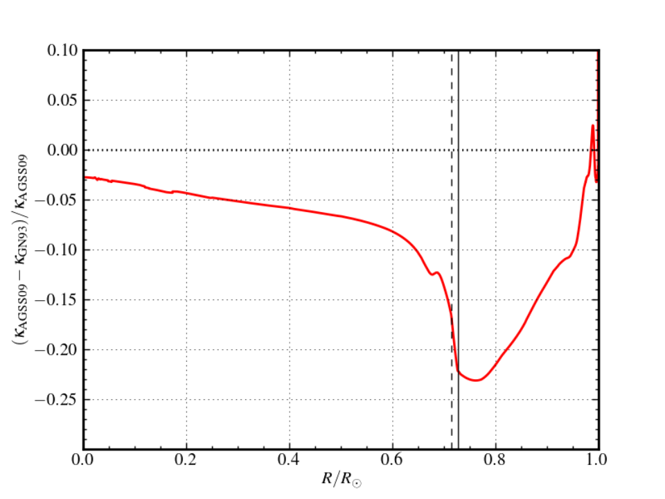
Figure 19: Difference in the opacity as a function of radius between two calibrated solar models, calculated with the cesam2k code with either the AGSS09 or the GN93 solar mixture. Vertical lines indicate the locus of the base of the convective envelope (AGSS09: continuous line, GN93: dashed line). - •
Change of opacity due to -elements enhancement.
The effect of an -elements enhancement on the age of globular clusters at very low [Fe/H] has been studied in several papers (see for instance Vandenberg & Bell, 2002; VandenBerg et al., 2012, and references therein). As an illustration, Fig. 20 shows that an enrichment in oxygen or in the other -elements produces cooler and fainter tracks in the HR diagram, which in turn induces a decrease of the age at turn-off. VandenBerg et al. (2012) have shown that the impact of oxygen is overwhelming in the age decrease, with at dex, a decrease of 1 Ga per step of dex in [O/Fe].
In Fig. 21, left panel, we have compared the turn-off age of stars of different masses with heavy elements mixtures of different [Fe/H] values ( and dex), and including either an -elements enhancement of dex or a solar -non enhanced- value dex. We used the BaSTI grids of stellar evolutionary tracks calculated for a constant value of (Pietrinferni et al., 2004). There is a general decrease in age with a maximum of 20 per cent for (solar) and 5 per cent at dex. The models enriched in -elements have a higher luminosity and the same initial hydrogen abundance, which turns into a smaller age.

Figure 20: Effect of an enrichment of oxygen and -elements on the MS turn-off. [From VandenBerg & Bell (2001).] - •
Change of opacity due to uncertainty on the metallicity.
In Fig. 21, right panel, we show that in case of the error on the metallicity [Fe/H] were of dex the TO ages would differ by up to per cent. A change of [Fe/H], at constant , in a stellar model has two main competing effects: (i) the helium abundance and therefore the mean molecular weight increases which tends to increase the luminosity, and (ii) the opacity increases which tends to reduce the luminosity. A smaller luminosity corresponds to an increase of age. In low-mass stars, the bound-bound and bound-free opacities, which play an important role, increase a lot when [Fe/H] increases. As a result, the luminosity is smaller and the TO age is higher. In high mass stars, where free-free opacities and scattering are more important, the opacity is less affected by an increase of metals. In these stars, due to the change of helium resulting from the [Fe/H] increase, the luminosity is higher and the turn-off age decreases.
- •
Change of opacity due to uncertainty on the He abundance or on .
To quantify the effect of changing the initial helium abundance of stellar models, we have compared the ages at turn-off of models calculated with initial helium contents of , and . We find that a decrease of from 0.28 to 0.25 induces a decrease of the turn-off age in the range 10 to 35 per cent for the interval of mass we considered (see Fig. 22, left panel). This is due to the fact that increasing also increases the mean molecular weight and in turn the luminosity. With a higher luminosity the age is smaller. Similarly, an increase of the ratio, from 2 to 5, produces a decrease of the turn-off age (see Fig. 22, right panel).
3.4 Equation of state
Depending on the location of the star or region of a star in the temperature-density plane, different contributions to the equation of state (EoS) have to be considered (top panel, Fig. 23). Prior to 1990, the equation of state used to calculate stellar models usually only included contributions from the ideal gas, degenerate electron gas, and radiation. Then in the early 90s, a leap forward has been accomplished, in the context of the work dedicated to the improvement of opacity, and more sophisticated EoS including the departures from ideal gas were made available. Both the OPAL EoS (Rogers & Nayfonov, 2002) and the MHD EoS (Nayfonov et al., 1999, part of the OP Opacity Project,) include the Coulomb effects, volume effects, and partition functions. We point out that during the last ten years, the numerical accuracy of these EoS has been improved.
Currently, stellar evolution codes use either the OPAL05 or the MHD EoS, which have been compared by Trampedach et al. (2006) and by Basu et al. (1999), this latter in the context of helioseismology. When necessary, for the modelling of dense very low mass stars, the dedicated EoS of Saumon et al. (1995) is used. Furthermore, several packages of EoS tables make a patchwork of the previous EoS, in order to cover the temperature-density plane as widely as possible. This is the case of Irwin’s FreeEos used in Cassisi et al. (2003a), and of the EoS used in the MESA code Paxton et al. (2011), see the top panel, in Fig. 23.
Taking into account the non ideal effects in the EoS changes the location of stellar models of low mass in the HR diagram (Fig. 23, bottom panel). More importantly the effects of the EoS can be probed by helioseismology through the modification they imply for quantities as the sound speed or the adiabatic index . Several EoS, among which the OPAL and MHD EoS, have been discussed and probed in the context of helioseismology (see for instance Guzik & Swenson, 1997; Basu & Christensen-Dalsgaard, 1997; Gong et al., 2001, and references therein).
The impact on the turn-off age of using two different EoS (OPAL and FreeEOS) has been evaluated by Valle et al. (2013) for a star with (metal rich globular cluster in the Large Magellanic Cloud). Their Table D.1 shows that the difference in age is lower than 1 per cent. Moreover, we considered the OPAL01 and OPAL05 versions of the OPAL EoS at solar metallicity and different stellar masses and found differences in the turn-off age that are lower than 1.5 per cent.


3.5 Microscopic diffusion
Microscopic (atomic) diffusion is the transport of chemical elements inside stars by different diffusion processes. In low mass K-G stars, transport by pressure (gravitational settling), temperature, and concentration gradients are dominant processes and the diffusion velocity of a species with respect to protons reads,
| (28) |
see Aller & Chapman (1960). In this equation is the relative concentration of ion in the mixture.
In hotter A-F stars, radiative forces have to be taken into account to explain abundance anomalies (Michaud, 1970; Turcotte et al., 1998; Alecian, 2007; Théado et al., 2012). This leads to add a term in Eq. 28 of the form
| (29) |
where is the local gravity and the radiative acceleration.

In low mass stars, on the MS, atomic diffusion transports helium and metals towards the centre (and depletes them in the envelope), while hydrogen is pushed up from the centre towards the envelope (see Fig. 24). On the other hand, in post SGB phase, during the first dredge up, the convection zone extends deep in the star and the resulting mixing kind of restores the initial abundance of metals at the surface, as confirmed by spectroscopic observations (Korn et al., 2006).
In models including microscopic diffusion, the envelope opacity increases due to the enhancement of hydrogen in the envelope. In turn, the envelope is deeper and the effective temperature is smaller as seen in the HR diagram of Fig. 25.
Atomic diffusion is a very slow process. Michaud et al. (1976) estimated the surface abundances depletion time scale,
| (30) |
and where is the mass in the convective envelope and is the temperature at its bottom. Table 4 lists the variation of with the mass of the star: the lower the stellar mass, the deeper the convective envelope, and the slower the process.
The increase of the central helium abundance (and therefore of the mean molecular weight), leads to an increase of the luminosity and therefore to a decrease of the duration of the MS. This is illustrated in Fig. 25, where we show that atomic diffusion reduces the age at turn-off of low-mass stars by a few per cent. This has consequences for the age-dating of globular clusters, the ages of which are reduced by Ga when diffusion is accounted for.
| 1.0 | 1.1 | 1.2 | 1.4 | |
| (Ga) | 5.4 | 1.5 | 0.11 | 0.0043 |
Furthermore, there are several possible formalisms to take atomic diffusion into account in stellar models, via the first term expressing the variation of chemical composition in Eq. 12 (see e.g. Burgers, 1969; Michaud & Proffitt, 1993; Thoul et al., 1994; Paquette et al., 1986, this latter provides coefficients for collisions). Thoul & Montalbán (2007) showed that with these different formalisms the diffusion velocities may change by up to per cent. As a consequence, the effect on age-dating is reinforced if the diffusion velocities are higher (Fig. 26).
Finally, the gravitational settling efficiency increases when mass increases because the convective zones are thinner. As a result, for masses higher than , there is a rapid quasi-total depletion of helium and metals at the surface of those stars, which is not observed. To properly model these stars, it is necessary to account for radiative forces in the calculation. Up to now, only two stellar evolution codes include radiative accelerations, the Montréal code (Richer et al., 2000) and the TGEC code (Théado et al., 2012). Other codes use recipes to prevent the full depletion (turbulence, mass loss, rotation).
4 Impact of stellar hydrodynamics (macrophysics) uncertainties on stellar ages
4.1 Convection
Heat and chemical element transport by convection play an important role in stellar evolution. When integrating the 1D equations for stellar structure, one only needs to determine where the medium is convective and how the temperature gradient is modified in the convective regions and their surrounding layers. The way these pieces of information are obtained is described in all text books of stellar structure and evolution. We provide here a brief overview.
4.1.1 Onset of convection
The onset of convection originates from a thermal instability due to buoyancy. Convection takes place whenever the radiative gradient is not able to transfer the energy efficiently enough. Let us consider a gravitationally stratified medium with both temperature and density and decreasing outwards. A blob of gas, which is slightly less dense (hotter) than the surrounding medium, rises up from its equilibrium position due to buoyancy. The Mach number of the medium, , \ie, the ratio of the convective velocity over the sound speed , is small ( from the bottom to the top of the solar convective region). One then assumes that pressure equilibrium is maintained between the ascending bubble and its surroundings. Then at a given level, say , above its initial position, the blob keeps on rising if it remains less dense than the surrounding medium (unstable stratified medium). In contrast, gravity pulls the blob back if it becomes denser (cooler) than the surrounding environment (stably stratified medium, see Fig. 27). The rising blob (density , temperature ) remains less dense (hotter) than the cooling medium () if the blob density decreases faster than that of the medium (its temperature decreases slower). This condition reads:
The condition for convective instability then is with for the medium and for the blob.
If the blob moves rapidly enough that its motion can be assumed adiabatic, , where is the ratio of the specific heat at constant pressure to the specific heat at constant volume and for an ideal monoatomic gas. Then the condition for the onset of convection becomes .
If the convection is inefficient, the temperature gradient of the medium remains nearly radiative hence . The reality lies in-between. The blob radiates energy during its motion, then . Convective heat transport decreases the temperature gradient of the medium, then . As a result, the medium is usually characterized by
| (31) |
The Schwarzschild criterion for convective instability in a homogeneous medium, can then be conveniently stated as
| (32) |
Both gradients are known at each level , regions which are unstable against convection are then easily identified in 1-D stellar evolutionary codes, in the framework of the mixing-length theory (Biermann, 1932). Furthermore, in presence of a -gradient, the criterion for convective instability becomes the Ledoux criterion (Kippenhahn et al., 2013, \eg,).

4.1.2 Location of convective regions in 1-D stellar models
The next issue then is where in a stellar model the criterion for convective instability (Eq. 32) is satisfied. Let us first consider the radiative gradient, (defined in Eq.9). It can also be written as
where is the total heat flux, the pressure scale height, the luminosity, and the thermal conductivity, all at level . In stars, convection can take place in the envelope, in the core, and in intermediate layers, mainly because or become large.
- •
Convective envelopes: for a given star (with a given total luminosity and total mass ), the opacity in the envelope (where the mass at level is ) is large due the presence of ions in partial ionisation zones, hence the radiative gradient is large. Moreover, in these regions the value of drops close to one and therefore becomes small. Both properties favour the onset of convection. As a consequence, cool stars do develop extended convective outer layers. The effective temperature, or the radius, depend on the properties of outer convection. Hence uncertainties in the description of inefficient convection in stellar models may affect the shape of the isochrones and accordingly the ages deduced from isochrone fitting.
- •
Convective cores: the ratio is quite large in the central regions when the nuclear energy rate strongly depends on temperature. This happens when the CNO cycle significantly operates, that is for MS stars of mass larger than about , depending on the chemical composition. Uncertainties in the location of the boundary of the central mixed region (see Sect. 4.2) involve variations of the lifetime of the central hydrogen burning phase and directly affect the ages.
4.1.3 Efficiency of convection
The properties of stellar convection are governed by the competition between several characteristic time scales: (i) the buoyancy driving time scale , where , the Brunt-Väisälä (BV) frequency, is the frequency associated to the oscillation of a perturbed parcel of a gravitationally stratified fluid (see lecture 2), (ii) the viscous time scale , and (iii) the radiative time scale . These latter quantities read,
| (33) |
where is the kinematic viscosity and a characteristic length scale. The Rayleigh number measures the strength of the instability
Both viscous and radiative effects inhibit the development of the instability. In stellar conditions such as in the Sun, the Rayleigh number () is huge and the instability leads to a strong driving.
On the other hand, the Prandtl number of the fluid measures the ratio of the thermal and viscous time scales:
In stellar conditions, is small () and the fluid can be considered as inviscid. As a consequence of the inviscid nature and of the large scales involved, the Reynolds number , is quite large. With the characteristic length scale , say m, and velocity , say , the solar Reynolds number is
much larger than the critical number () beyond which turbulence sets in. Stellar convection is highly turbulent with a wide range of spatial scales involved (Kupka, 2009, \eg,).
As shown by 3-D simulations by \eg Stein & Nordlund (1998), the convective motions in stellar envelopes show narrow cool descending plumes and hot rising bubbles, both types of motions penetrating in the adjacent stably stratified layers. In 1-D stellar models, however, the description of convection, the “mixing length theory” (MLT), is based on a very simple picture. It assumes that a blob which is less dense than the surrounding medium rises up to a level where it dissolves giving back its energy excess to the medium. The distance is the mixing length and is usually taken as a fraction of the pressure scale height, , that is .
When convection takes place somewhere, its impact depends on its efficiency. A measure of the efficiency is given by the ratio of the thermal time scale to the buoyancy time scale. is also the product of the Rayleigh number by the Prandtl number (Canuto et al., 1996). The quantity
| (34) |
measures the ability of convection to transport heat. The efficiency can then be either large or small. An inefficient convection however does not mean that the convective flux is small.
In stellar envelopes, convection is inefficient () at the top of the convection zone. The superadiabatic gradient defined as the difference between the actual gradient and the adiabatic one is proportional to the squared mixing-length parameter:
In convective cores, convection is quite efficient and the actual gradient is close to adiabatic whatever the mixing-length value. On the other hand, non-local effects generate overshooting beyond the Schwarzschild limit. This adds a new free parameter, the overshooting distance . Therefore, the implementation of turbulent convective transport in 1-D stellar codes remains one major weak point of stellar evolution theory. Over the years, many tentative works have aimed at extending the phenomenological description proposed by Böhm-Vitense (1958) after the work of Prandtl (1925). Despite these efforts, the MTL including its improved variants (see below) basically remains in use in the current stellar evolutionary codes.
4.1.4 Convective gradient
In stellar convective regions, one needs to determine the actual temperature gradient, . It is derived from the total flux conservation law , where the total flux is known at each level :
The radiative flux depends on the unknown temperature gradient
One also needs the convective flux . Assuming pressure equilibrium, the convective flux is identified with the enthalpy flux and is therefore defined as
where are the temperature deviations from the horizontal mean , and the counterpart for the vertical velocity. Because of the turbulent nature of the convection, one must compute an ensemble average of the statistical fluctuations of velocity and temperature with respect to a static background. In order for turbulent convection implementation to be tractable in a 1-D stellar code, several assumptions and approximations, listed belowr, have to be made.
- •
Convection can be assumed to be incompressible because the Mach numbers are small (). Actually, pressure and density fluctuations with respect to the averaged background are neglected except for the density fluctuation entering the source of convective instability, \ie, the buoyancy acceleration .
- •
The second assumption is that of a stationary flow. All quantities are considered as statistical averages. This is justified by the fact that the dynamical time scales of relevance for turbulent convection are much shorter than the evolutionary time scale for MS stars.
- •
The turbulence is assumed to be isotropic and homogeneous. The relevant quantities are horizontally averaged. A better description ought to include the horizontal heat exchange between rising, hotter blobs and cooler, descending plumes.
- •
, that is the product of mean velocity times mean temperature difference between the blob and the surrounding at the time of dissolution.
- •
Convection in 1-D stellar models is local, that is the convective gradient at a given level is written in terms of quantities defined at the same level. This is a strong assumption, which is not justified. One consequence is a non-physical treatment of the boundaries between radiative and convective regions. They are imposed by the Schwarzschild criterion, which does not allow for convective penetration into the neighbouring radiative layers.
- •
The motion of the blob is assumed to stop after some travel distance where it gives back its heat excess to the medium. The distance is taken to be some fraction of . This fraction is a free parameter, which makes the formulation non predictable. In the solar case, this distance is derived from a calibration process because the solar model must match its independently known mass, luminosity, and radius, at its current age. The value however depends on the physical inputs used to build the solar model. There is no reason that the same value applies to another star with a different mass, chemical composition, and age. Actually, 3-D numerical simulations of stellar envelopes show that the mixing length should vary across the HR diagram (Magic et al., 2014, \eg,). This is confirmed by seismic studies of a few stars (Miglio & Montalbán, 2005, see \eg,).
- •
Turbulent pressure, turbulent kinetic energy are discarded. 3-D simulations however show that they are not negligible (Rosenthal et al., 1999; Robinson et al., 2003; Trampedach, 2004).
With the above assumptions, using conservation of the flux and of the energy, it is possible to derive a local relation between the convective flux and the superadiatic gradient () such that
where is a function of the efficiency (Eq. 34), and depends on the equilibrium stratification properties.
In the formulation of Böhm-Vitense (1958), the heat is assumed to be transported by one eddy-size blobs (\ie, corresponding to one single spatial turbulent scale). Although this is an unjustified assumption, the resulting formulation was and still is the one implemented in most 1-D stellar codes to compute the temperature gradient in regions of superadiabatic (\ie, inefficient) convection. An improved formulation by Canuto & Mazzitelli (1991, hereafter CM) and Canuto et al. (1996, hereafter CGM) takes into account the multi-spatial scale nature of stellar convection (Full Spectrum of Turbulence, FST). It has been implemented in a few stellar codes. As a result, the dependency of the flux on the efficiency, \ie, the function , differs between the two descriptions MLT and FST.

Figure 28 from Canuto et al. (1996) shows the ratio of the efficiency dependency of the CGM approach to that of the MLT as a function of the logarithm of the efficiency . The departure from one is the consequence of including the whole spectrum of kinetic energy in the FST convective flux. The plot shows that the MLT underestimates the convective flux for high efficiency and overestimates it for small efficiency.
For an efficient convection () , one has:
For an inefficient convection, ()
Comparisons with observations show that the FST represents an improvement over the MLT (Gabriel, 1995; Mazzitelli et al., 1995). However it suffers from the same other limitations as the MLT, particularly this is a local theory which depends on a free parameter, the mixing length.
4.1.5 Convection in stellar envelopes
In the MLT description, the efficiency is given by
where is related to the efficiency as . Because of the opacity peak in partial H ionization regions, near the superadiabatic layer (SAL), the opacity is large. As a consequence, and the instability generates a strong driving. But is small in the outer layers and despite the strong driving. Convection is therefore inefficient in envelopes of cool stars. The temperature gradient then is intermediate between the radiative and the adiabatic gradient. For small efficiency, the gradient writes
| (35) |
see \eg Böhm-Vitense (1958); Böhm-Vitense (1992). The convective flux carries little energy
Impact of the mixing-length value on the temperature gradient.
Left panel of Fig. 29 shows the run of the superadiabatic gradient as a function of the temperature in the outer layers of a model for two values of the parameter and . From Eq. 35, one obtains:
For a given stratification, the mixing-length value determines the magnitude of the efficiency and therefore the gradient: the larger , the larger the convective efficiency and the farther the gradient from the radiative one. The convective efficiency is small but the driving is strong hence the actual gradient in presence of convection is much larger than the adiabatic one and closer to, although significantly smaller than the radiative one. How smaller depends on the value one adopts for the mixing-length parameter.
Below the SAL (up to , for the model), the convection becomes quite efficient, \ie, , because becomes large. For a large efficiency, one has
The larger , the larger the efficiency and the smaller the actual gradient compared to the radiative one, the closer to the adiabatic one.
Impact of the mixing-length value on evolutionary tracks.
The right panel of Fig. 29 shows the effect of increasing on the evolutionary tracks in the HR diagram. The impact depends on the effective temperature, hence on the mass at a given luminosity. Stars of hotter than are not impacted as can be seen for the tracks. The reason is that the outer convection region is too thin and not dense enough to play an important role in the energy transport.
The comparison of the tracks on the other hand shows that there is a clear shift of the higher track toward the blue for models at the same evolutionary stage, \ie, with the same value of central hydrogen abundance. For a larger , the star is more compact, the radius is smaller, and is higher at the same luminosity. Hence, for low mass stars (), an increase of causes an increase of .
Uncertainty on the mixing-length value: impact on TO ages.
Figure 30 compares the age at TO of a reference model with solar composition and solar value with the TO ages of models computed assuming dex. The maximum effect of a change of by dex on the TO age occurs in the mass range . A maximum difference of 3 per cent is found at . The impact is therefore small. The small impact on isochrones has been shown by Castellani et al. (1999).
FST versus MLT: impact on TO ages.
As mentioned above, the FST theory provides an improved model of turbulent convection. That leads to a different prescription of the convective flux with respect to the standard MLT one. Nevertheless, the FST remains a local theory, which also requires the definition of a mixing-length scale. Either (where is the distance to the convection boundary and is the pressure scale-height at the top boundary), or are used. The free parameters , , or are calibrated to fit the solar radius at solar age. Their values depend on the convective flux description, but also on input physics such as opacity, solar mixture, EoS, and atmospheric boundary conditions (BC), see \eg, Bernkopf (1998); Montalbán et al. (2004); Samadi et al. (2006). For instance, for a given set of microphysics and BC, we could match the current Sun with either , , or . However, because of the different dependence of the convective flux on the superadiabaticity, evolution in the HR diagram with a constant value is not equivalent to the evolution of a model of same mass with a constant value of . As shown in left panel of Fig.31, while yields a similar radius than CGM during the MS of a one solar mass model, its value must be increased to during the RGB to mimic the same convective efficiency than the CGM treatment.


A comparison assuming the solar calibrated values and (Fig. 31, bottom panel) indicates that the impact on age at turn-off is small (ageage per cent). The maximum impact occurs for masses in the range . The impact on isochrones is small, for a constant free parameter ( or ). This remains true for isochrones with low metallicity used to reproduce globular clusters. This is illustrated in Fig. 32, left panel, in the case of M92 (Mazzitelli et al., 1995; Montalbán et al., 2001, \eg,).
Calibrations of the mixing-length value.
Figure 32 (right panel) shows the variation of the value derived from 3-D surface convection simulations in a diagram for evolutionary tracks of various masses and a solar chemical composition (Trampedach & Stein, 2011). For a one solar mass for instance, the value roughly varies from to on the MS. For ZAMS models with masses decreasing from 5 to , increases from to .
One then needs to calibrate the value across the HR diagram. This can be obtained with a prescription for the value derived from 2-D or 3-D numerical simulations (Ludwig et al., 1999; Ludwig et al., 2008; Trampedach & Stein, 2011; Magic et al., 2014). An alternative is to use patched models, which are built as a 1-D stellar interior with the outer layers originating from a 3-D simulation (Rosenthal et al., 1999; Straka et al., 2006; Samadi et al., 2010). An observational calibration can also be directly obtained on a case by case level by performing à la carte seismic studies (see lecture 2).
4.2 Overshooting from convective cores
MS stars of masses develop a convective core because of the high temperature dependence of the nuclear CNO cycle. Convection in the dense central layers is very efficient and the temperature gradient is nearly adiabatic. As a consequence, the value of the mixing length has no effect on the properties of the convective core.

Figure 33 (left panel) shows the temperature gradients , , and the actual gradient , as a function of fractional mass, in the central regions of a MS model. The convective core extends over the inner 12 per cent in mass. The radiative gradient sharply decreases with radius and reaches the adiabatic gradient at a radius defined as the Schwarzschild radius . In the convective region, the temperature gradient , which is required for transporting the energy (or luminosity) remains close to , namely the difference is small and remains of the order of independently of the value of the mixing length. On the other hand, core overshooting is expected to occur in stars. It consists in convective elements moving over into the radiation layers above the convective core (see \eg, Dintrans, 2009, for a review). However this process is poorly understood and crudely modelled in stellar evolutionary codes (see Chiosi, 2007, for a review).
Indeed the transition between the convective core and the radiative region above is delimited by the Schwarzschild criterion (\ie, ). This corresponds to the location where the acceleration of the convective motion vanishes. Because of inertia, the moving fluid keeps on travelling over some distance into the adjacent radiative region. During its travel, the bubble is decelerated till its velocity vanishes. This induces mixing of chemical elements and heat transport in the overshooting region, and a modification of the corresponding gradients in the region above the convective core. To evaluate the overshooting distance properly, a non-local description of convection is necessary. Instead, a crude formulation is often used, which states that the overshooting distance simply is some fraction of the pressure scale height, .
In order to avoid some incoherence when the convective core is quite small (for instance in low-mass stars), the overshooting distance is often actually set to be a fraction of , or of the core radius if the latter is lower than . In addition, in the overshooting region it is often assumed that the matter is fully mixed and that the temperature gradient is the adiabatic one (see Fig. 33, right panel).
Several important open questions/issues remain:
- •
What is the size of the zone of extended mixing? The parameter is a free parameter of models. The question is to know whether it depends on the mass, metallicity, or other properties of the star.
- •
Is the stratification fully adiabatic in the overshooting region?
- •
What kind of chemical mixing does actually occur? Is it instantaneous or diffusive?
Convective core overshooting widens the MS, which modifies the shape of isochrones. Therefore, one way to quantify overshooting has been to try to fit the observed isochrone MS turn-off of open clusters, and the width of the MS band of groups of stars (Maeder & Mermilliod, 1981; Andersen et al., 1990; Stothers, 1991; Schaller et al., 1992; Lebreton et al., 2001; Cordier et al., 2002, see \eg,). Furthermore, insights on how the overshooting distance varies with stellar mass, metallicity, and evolutionary state were obtained by the modelling of samples of binary stars of known mass and/or radius, and chemical composition (Andersen et al., 1990; Ribas et al., 2000; Claret, 2007). Different empirical calibrations of the overshooting distance suggest that it roughly covers the range . However, the value depends on the model input physics. For instance, Schaller et al. (1992) showed that the improvement of opacities implies a decrease of from to .


4.2.1 Impact of overshooting on stellar age
Including core overshooting in the modelling increases the size of the mixed core. As a result, on the MS, more hydrogen is available for nuclear burning. This lengthens the MS phase and yields older models at TO. This is clearly illustrated in Fig. 34 (left panel), which shows the evolution of the size of the mixed central region (in relative mass) as a function of the central hydrogen abundance (a proxy for the age) for two models, one without core overshooting and the other with core overshooting of . Fig. 34 (right panel) shows a HR diagram comparing evolutionary tracks without overshooting to tracks including core overshooting of , for masses in the range . Comparison of the location of the TO for the two types of tracks evidences the lengthening of the MS by about 20 per cent when a core overshooting of is included.


4.2.2 Overshooting of convective cores: the age of the Hyades
As just discussed, the end of the MS for a given stellar mass occurs at lower effective temperature and higher luminosity when core overshooting is included. Accordingly, the shapes of the isochrones, which have turn-off masses larger than are significantly modified. This modifies the age of rather young open clusters. This is the case of the Hyades, the closest ( pc) and well-studied open cluster which has turn-off masses in the range (see Fig. 35). With an overshooting amount of , the isochrone fit gives an age of Ma, whereas when no overshooting is assumed, the derived age is Ma (Fig. 35 right panel). The relative age difference in this case amounts to 13.6 per cent.
Note that seismic studies of stars at TO could provide constraints for core mixing. Interesting candidates are the Tau binary system components, which are -Scuti stars of known mass located in the vicinity of the Hyades TO. However their fast rotation will make the task difficult.


4.2.3 Vanishing convective cores
As discussed above, for masses larger than (the exact mass depending on the chemical composition) the convective core is well developed. On the other hand, convective cores begin to form at . In the intermediate mass range, \ie, , the problem is how to treat overshooting of very small convective cores.
The simplest case is to assume no overshooting for masses and an overshooting of for masses . A typical case is to take and . More sophisticated prescriptions have been proposed by, for instance, Pietrinferni et al. (2004), but see also Bressan et al. (2012), who considered variations of the overshooting parameter with mass, as schematically represented in Fig. 36, right panel. In their first option (case A), linearly increases with the model mass from at to at . In their case B, also linearly increases with the model mass from at to at , but with a change of slope at . The third option, adopted in the BaSTI code, is intermediate between case A and B, \ie, no overshooting for masses lower than , then an overshooting at , followed by a linear increase of until it reaches at . The impact of these different options on a 5.5 Ga isochrone is shown in Fig. 36 (right panel). There are little differences between the BaSTI case, case B, and the case with no overshooting. On the other hand, for the case A option, overshooting is larger and the maximum amount of overshooting is reached earlier, at . To match the same TO location, in case A, an isochrone would have to be older than in the other cases.
4.2.4 Impact on ages at MS turn-off
Figure 37 shows the relative differences in age at turn-off between models including a core overshooting of and the reference models (no overshooting). For models with masses below , the convective core is quite small, hence the core overshooting distance and its impact on the age are negligible. For models with masses higher than , the core overshooting is no longer negligible. The impact on age amounts to about 30 per cent in a model. It decreases with the mass of the model but still equals per cent at . The decrease of the impact with the mass of the turn-off models is due to a decrease of the pressure scale height of the central layers with the model mass.
4.2.5 Modelling overshooting of convective cores: alternatives
The large uncertainty of the core overshooting extent is a severe flaw for stellar models at least when the age-dating is concerned. This is why other ways to model core overshooting have been proposed as more realistic alternatives. One can mention for instance:
- •
Diffusive overshooting. This approach assumes that convective velocities decrease exponentially from a level located inside the Schwarzschild convective core, beneath its upper boundary, to a level located up in the radiative region (Deng et al., 1996; Ventura et al., 1998; Zhang & Li, 2012; Zhang, 2013). This adds a diffusion coefficient in Eq. 12. When the classical non diffusive overshooting is assumed, models of low-mass stars (in particular the solar model) develop a convective core at the end of the PMS, which may remain on the MS. Small cores then require a special treatment (Sect. 4.2.3), not necessary in the diffusive approach. For more massive stars, there are no differences between the diffusive and non diffusive treatments on the MS, but evolved stages like He-burning may be affected (Ventura et al., 2005).
- •
A prescription derived from energy conservation principles has been derived by Roxburgh (1978); Roxburgh (1989). This prescription allows the estimate of an upper limit to the extent of overshooting from convective cores. Numerical estimations (Roxburgh, 1992) suggest that the mass of the extended convective core is proportional to the mass of the Schwarzschild convective core (). This approach does not provide the right amount of overshooting (as estimated from observations) unless the dissipation of energy is included but dissipation is a major unknown (Roxburgh, 1992; Roxburgh & Simmons, 1993; Maeder, 2009; VandenBerg et al., 2006, \eg,).
- •
Overshooting due to plumes, based on an assumption of universal turbulent entrainment. A theoretical prescription can be derived, which involves several parameters (Zahn, 1991; Rieutord & Zahn, 1995; Lo & Schatzman, 1997, \eg,).
- •
Several variants of a non-local description (Reynolds stress model) using moment equations and closure models (Xiong, 1978; Xiong, 1985; Grossman, 1996; Canuto & Dubovikov, 1998; Canuto, 1999; Zhang & Li, 2012, \eg,).
Unfortunately, all these formulations involve one (or more) free parameters. Some progress will come from prescription and/or calibration with 3-D simulations, although this currently remains somewhat difficult (Meakin & Arnett, 2007; Gilet et al., 2013; Staritsin, 2013; Viallet et al., 2013, \eg,).
4.3 Rotation
Stars rotate and their surface rotation velocity is known to change with time (see R. Jeffries’ lecture). That can be the consequence of angular momentum loss by external torques (for instance magnetic braking, coupling with an accretion disc), and of structural changes such as core contraction and envelope expansion during MS and post-MS evolution. The physical processes linked with rotation and its evolution are manifold and interconnected. This makes the treatment of rotation in stellar evolution modelling very complex (Maeder et al., 2013; Meynet et al., 2013; Mathis, 2013, \eg,). Several books and reviews deal with the effect of rotation on stellar structure and evolution (see \eg, Maeder & Meynet, 2000; Tassoul, 2007; Maeder, 2009; Palacios, 2013; Goupil et al., 2014, and references therein).
First of all, rotation breaks the spherical symmetry of stars and therefore creates a thermal imbalance. As a result, large-scale circulation (meridional circulation) takes place that transports chemicals and angular momentum (AM). Since the resulting rotation regime is not uniform (), the vertical and horizontal shear induced by differential rotation give rise to various hydrodynamical instabilities, which generate turbulence and hence transport angular momentum and chemicals. The turbulent transport (mainly the horizontal one) in turn modifies the efficiency of large-scale transport and the final rotation profile.
The effects of the interaction between magnetic fields and rotation are also manifold. The interaction between convection and rotation leads to the generation, by a dynamo mechanism, of a magnetic field, whose intensity seems to be linked with rotation. On the other hand, this magnetic field may channel stellar winds to large distances (as in solar-like stars), increasing the loss of angular momentum from the stellar surface and braking the star. In radiative zones, magnetic fields can freeze plasma motions and also induce magnetohydrodynamical instabilities (for instance the Taylor-Spruit instability) that may affect the transport of angular momentum and chemical elements.
Finally, the propagation of internal gravity waves22 2 These waves are excited at the boundaries of convective zones and propagate in the gravitationally stratified radiative zone where they extract or deposit AM. (IGW) in a rotating medium can also lead to AM transport and modify the internal rotation, and in turn chemical composition profiles.
To summarize, rotation interacts with many physical processes which may transport AM and matter, in a complex way. These interactions are currently addressed in many theoretical studies (Maeder et al., 2013; Meynet et al., 2013; Mathis, 2013, see \eg,) and benefit from the results of 3-D numerical simulations (Browning et al., 2004). Resulting modifications of internal angular velocity and chemical composition profiles may strongly affect age-dating.
4.3.1 Angular momentum transport and rotational mixing in stellar models
Here, we only briefly summarize the main aspects related to model calculation.
Concerning the AM transport, two main approaches have been followed. The first one, proposed by Endal & Sofia (1976), consists in treating both AM and chemical transport as diffusive processes; the problem is then reduced to 1-D (Pinsonneault et al., 1989, see also). In the second approach, the AM transport is treated as an advective-diffusive process, while the transport of chemical elements obeys a diffusion equation. In that context, Zahn (1992) assumed that the turbulence induced by differential rotation is stronger in the horizontal direction than in the vertical direction, which implies that the angular velocity is about constant on isobars. This behavior justifies the hypothesis of so-called shellular rotation, which leads to express any quantity as a function of pressure only, or of radius provided the rotation is slow (Maeder & Zahn, 1998, see also).
In the framework of shellular rotation, the transport of angular momentum in radiative zones obeys an advection-diffusion equation that reads,
| (36) |
where is the local specific AM and is the AM flux, both at level , and is the time derivative of the radius. The AM flux is the sum of several contributions to be evaluated. In convective zones the angular momentum is assumed to be constant, that is convective zones are assumed to rotate like solid bodies. This assumption has been investigated in some specific cases (Palacios et al., 2006).
In order to solve Eq. 36, one has to specify the surface AM losses . For stars with convective envelopes, the surface AM losses are assumed to result from magnetic braking by stellar winds (Schatzman, 1962; Mestel, 1968). One has also to specify the initial AM profile across the star. It is commonly assumed that stars rotate like solid bodies at the beginning of the PMS and as long as they remain entirely convective. On the other hand, the surface rotation is assumed to remain constant and equal to the rotation of the protostellar disc as long as disc locking occurs.
The total AM flux, results from several AM transport processes (Talon, 2008; Maeder, 2009, \eg,). It is given by , where the currently identified contributions are:
- •
: the AM transport by meridional circulation. reads, , where is the vertical velocity of the meridional circulation.
- •
: the AM transport by the turbulence generated by different kinds of instabilities taking place in the radiative regions. The combined effects are modelled as a diffusive process and contribute to a total turbulent viscosity . The AM flux then reads .
- •
: the AM transport by IGW in stellar radiative regions has been proven to be efficient to transport AM and to influence the chemical mixing (Schatzman, 1993; Charbonnel & Talon, 2005, \eg,). The determination of an accurate expression for the IGW, AM flux is nowadays the object of intense theoretical research (Talon, 2008; Palacios, 2013, see \eg,).
- •
: the AM transport in presence of a magnetic field. The torque of the Lorentz force, magneto-hydrodynamic instabilities (as the Taylor-Spruit instability), and multi-diffusive magnetic instabilities may slow down the star and lead to rigid rotation. The efficiency of these mechanisms to slow down the radiative regions of solar-like stars and giant stars depends on its modelling, which remains debated (Strugarek et al., 2011; Garaud et al., 2013; Cantiello et al., 2014).
The turbulence induced by shear instabilities is strongly anisotropic. The vertical transport of chemicals elements due to rotation (rotational mixing) in radiative zones can then be modelled by a diffusion process resulting from the interaction between the meridional circulation and the shear turbulence (Chaboyer & Zahn, 1992). Therefore, a diffusion coefficient is added to the total diffusion coefficient in the equations of evolution of the chemical abundances (Eq. 12). Convection zones are assumed to be homogenized on very short time-scales (\ie, instantaneously).
The transport coefficients , , , and couple up the evolution of AM with the evolution of chemical elements. For instance, explicitly depends both on the vertical velocity of the meridional circulation and of the turbulent viscosity. While prescriptions for these coefficients exist (Mathis, 2013, for a review, see), they however suffer from several uncertainties (Meynet et al., 2013; Maeder et al., 2013).
4.3.2 Impact of rotationally-induced mixing on stellar structure and isochrones
As mentioned above, rotationally-induced mixing refuels the core with fresh hydrogen. Therefore, at a given evolutionary state, that is for a given value of , the mass of the mixed core is larger. As a result, as illustrated in left panel of Fig. 38, the higher the rotation rate, the longer the MS duration. The effect of rotationally-induced mixing on isochrones can be seen in Fig. 38, right panel: at a given age, when rotation is included, the TO mass is higher and the TO sits at higher effective temperature, which affects the age-dating.


4.3.3 Rotationally-induced mixing versus convective core overshooting
Several sets of evolutionary tracks calculated with different options, \ie, shellular rotation, overshooting or both, can be found in the literature: for instance for a model (Talon et al., 1997), a model (Eggenberger et al., 2010a; Marques et al., 2013), or a model (Goupil & Talon, 2002), but see also the book by Maeder (2009). The conclusion of these studies, illustrated in Fig. 39, is that for masses above , the effect on the MS of rotationally-induced mixing is roughly equivalent to the effect of a core overshooting of . This result is consistent with the result of a 3-D numerical simulation of a rotating convective core for a A-type star (Browning et al., 2004).
However, the confrontation of models to observations indicates that rotational mixing is not sufficient to reproduce the MS width, which makes additional core mixing necessary. Therefore stellar models have to include both shellular rotation and core overshooting. As discussed by Ekström et al. (2012), the comparison with rotation velocity measurements in young B-stars by Huang et al. (2010) provides a prescription for the initial rotation velocity, that is where is the break-up velocity (velocity corresponding to a balance between gravitational and centrifugal accelerations). Moreover, Ekström et al. (2012) proposed a prescription for the amount of overshooting necessary to match the observed MS-width:
- •
no overshoot for ,
- •
for
- •
for .
Therefore, in presence of rotationally-induced mixing with the necessary amount of core overshooting on the MS () is smaller than in the case without rotation (, see Sect. 4.2), while the theoretical and observed MS-widths better agree when rotationally-induced mixing is accounted for. Note also that in order to reproduce the effects of rotationally-induced mixing both on the MS and post-MS evolutionary tracks, the value of the overshooting parameter must vary in models accounting for overshooting only (Eggenberger et al., 2010b).
A similar comparison has been carried out for 1.58 Ga isochrones by Girardi et al. (2011): a synthetic HR diagram was populated by stars distributed according to an IMF and isochrones assuming either and , and , or and . The impact of the rotation and/or overshooting is visible on the shape of the isochrone at the turn-off.
4.3.4 Impact on TO ages
To estimate how rotationally induced mixing affects stellar ages, we used the data provided by the Geneva team (Ekström et al., 2012) to compare the ages at TO of models including shellular rotation with an initial rotational velocity of with the ages of models without rotation. In both cases, the Geneva grids include overshooting according to the prescription given in Sect. 4.3.3. The results are shown in Fig. 40. The TO ages differ by up to 30 (25) per cent for . For , the MS-lifetime increase remains the same for any mass, \ie, scales as . The impact is smaller (a few per cent) for stellar masses below . The large increase of the age difference between and is attributed to the fact that the convective core does not appear at same age for a given mass whether rotation is included or not. We obtained similar results using the STAREVOL grids (Lagarde et al., 2012).
Finally, let us add that MS stars of mass use to rotate fast. Fast rotation may change the aspect ( and ) of the star, depending on rotational velocity and inclination angle (Pérez Hernández et al., 1999, see \eg,). In turn, the shape of the isochrones can be modified (independently of rotational mixing), which may further affect age-dating (Lebreton et al., 2001, see \eg Fig. 13 in).
5 Conclusion
The most appropriate method to obtain accurate stellar ages relies on the computation of stellar models. However these models are far from being perfect, they are affected by several sources of uncertainties. Some of them are well-known, some are difficult to identify. It is then not easy to provide ages with realistic error bars. With the nowadays, high-quality, ground and space data, efforts are made to identify and quantify the most important biases affecting stellar age-dating. The ultimate goal is to eliminate them.


In that respect, in the framework of the scientific preparation of the CoRoT mission, a European working group, ESTA-CoRoT, was in charge of carrying out in-depth comparisons of stellar models (Monteiro et al., 2006; Lebreton et al., 2008b; Lebreton et al., 2008a; Montalbán et al., 2008, see \eg,). The group has compared models calculated with ten different stellar evolutionary codes. Prescriptions had been given to have, as far as possible, the same input physics, physical constants, and astronomical constants in all codes. The model comparisons were made for several cases corresponding to different choices of the mass, initial chemical composition, and evolutionary stage (Monteiro et al., 2006; Lebreton et al., 2008b, for more details see). These cases were chosen to be representative of the CoRoT seismic targets. The position in the HR diagram of one of the sets of models that have been compared is shown in Fig. 41. In Fig. 42 we show the comparisons of the radius, luminosity, effective temperature, and age of the models calculated by each participating code with the results obtained with the cesam2k code (Morel & Lebreton, 2008). The left panel shows the mean relative differences in these quantities, while the right panel displays the maximum differences. Concerning the age, the mean differences are in the range per cent, while the maximum differences are in the range per cent, which is quite high. However, if we only consider the codes that strictly followed the prescriptions for the comparison, that is adopting exactly the prescribed input physics and constants (blue symbols in Fig. 42), the differences are reduced by a factor of about two. In this case, we can consider that the differences between the code results are only due to differences in numerical treatments, that is the handling of table interpolation (to get the opacity, EoS outputs, etc.), the methods used to solve the equations, and hidden numerical mistreatments (time steps and mesh points, convective boundaries, etc.). The thorny problem of the numerical determination of convective boundaries has been addressed recently by Gabriel et al. (2014). More generally, numerical treatments are discussed in detail in \eg, Lebreton et al. (2008a); Montalbán et al. (2008); Lebreton & Montalbán (2010), and references therein.
In the present lecture, our approach has been to use the same evolutionary code (cesam2k) to estimate the impact of different physical inputs on the TO age value. The results are synthesized in Fig. 43, which highlights the huge impact of, on the one hand, the uncertain value of the initial helium abundance, and, on the other hand, the uncertain amount of mixing induced by overshooting and rotation, which determines the quantity of fuel available on the MS.
To better visualize the domain of mass and age concerned by model uncertainties, we show in Fig. 44 the TO mass of observed stellar clusters of different ages, while in Fig. 45 we indicate the domain of mass associated to the different uncertainties in the model inputs. We stress that the model uncertainties do not add up linearly, but correspond to the variation of one process at a time. Monte Carlo techniques can be used to estimate the cumulative effect of all sources of uncertainties (Chaboyer et al., 1992; Valle et al., 2014, \eg,).
Actually, different input physics are used in different stellar evolution codes. As a result, different stellar ages are inferred from different grids of models. Gallart et al. (2005) compared evolution tracks of a star in the HR diagram provided by the BaSTI group (Pietrinferni et al., 2004) and by the Padova group (Girardi et al., 2002) and found that the same TO position is reached by isochrones of ages differing by 30 per cent (see Fig. 46, left panel). This quite significant difference is attributed to several differences in the model inputs, in particular overshooting (Pietrinferni et al., 2004). Gallart et al. (2005) also compared the ages of metal-deficient stellar populations that would be predicted by different sets of model isochrones for three given choices of the pair (TO location, subgiant position). As shown in Fig. 46 right panel, the differences in age are more important for older stars: at ages of Ga the predicted ages differ by per cent, while for older stars (ages of or Ga) the ages differ by per cent. The differences are attributed to different model input physics (atomic diffusion, overshooting, microscopic physics).
To summarize, the present lecture showed that the physical description of stellar models must still be significantly improved in order to provide accurate ages of MS stars at a precision level better than 20 per cent. We could not discuss here all the processes which can affect the age determination. While the impact of numerics, input chemical composition, and microphysics can be estimated rather easily, the impact of macrophysics is much more difficult to estimate because its description involves processes which are not well described, imply many parameters, and are sometimes even unidentified. Furthermore, the present lecture focused on MS stars, therefore the sources of uncertainties on the time elapsed during advanced stages of stellar evolution have not been evaluated.
Accurate ages at the level of 20 per cent or less for low mass MS stars are required in many astrophysical fields like the formation and evolution of planetary systems or the evolution of the Galaxy. This need will be even more crucial when high-quality space data provided by, \eg, the PLATO-ESA mission (Rauer et al., 2013) and the Gaia-ESA mission (Perryman et al., 2001) will be available. Improving the physical description of stellar models is then certainly worth the effort. The observational progress will have to be supported by theoretical and experimental developments, and by numerical simulations in 2-D and 3-D. For instance, recent progress came from the the building of patched 1-D stellar models which include the convective outer layers obtained from 3-D simulations (Samadi et al., 2012), and from 2-D rotating models such as those calculated with the ROTORC code (Deupree, 1995) and the ESTER code (Rieutord & Espinosa, 2013).
Acknowledgements
The authors would like to thank the “Formation permanente du CNRS” for financial support. The preparation and writing of these lectures largely benefited from the use of the SIMBAD database, operated at CDS, Strasbourg, France and of the NASA’s Astrophysics Data System. Elements of these lectures have been presented in 2007 at the ESA ELSA School on the Science of Gaia in Leiden, The Netherlands, by Y. Lebreton (unpublished), in 2008, at the International Young Astronomer School on CoRoT Astrophysics in Meudon, France, by Lebreton & Montalbán (unpublished), and, in 2009, at the EES 2009 CNRS School in Aussois, France (Lebreton & Montalbán, unpublished).
References
- Adelberger et al. (2011) Adelberger, E. G., García, A., Robertson, R. G. H., et al. 2011, Rev. Mod. Physics, 83, 195
- Alecian (2007) Alecian, G. 2007, in Stellar Evolution and Seismic Tools for Asteroseismology - Diffusive Processes in Stars and Seismic Analysis, EAS Publications Series, Vol. 26, C. W. Straka, Y. Lebreton, & M. J. P. F. G. Monteiro (eds), p. 37
- Aller & Chapman (1960) Aller, L. H. & Chapman, S. 1960, ApJ, 132, 461
- Alves-Brito et al. (2010) Alves-Brito, A., Meléndez, J., Asplund, M., Ramírez, I., & Yong, D. 2010, A&A, 513, A35
- Andersen et al. (1990) Andersen, J., Clausen, J. V., & Nordstrom, B. 1990, ApJ, 363, L33
- Angulo et al. (1999) Angulo, C., Arnould, M., Rayet, M., et al. 1999, Nuclear Physics A, 656, 3
- Asplund et al. (2005) Asplund, M., Grevesse, N., Sauval, A. J., Allende Prieto, C., & Kiselman, D. 2005, A&A, 435, 339
- Asplund et al. (2009) Asplund, M., Grevesse, N., Sauval, A. J., & Scott, P. 2009, ARA&A, 47, 481
- Aver et al. (2013) Aver, E., Olive, K. A., Porter, R. L., & Skillman, E. D. 2013, JCAP, 11, 17
- Badnell et al. (2005) Badnell, N. R., Bautista, M. A., Butler, K., et al. 2005, MNRAS, 360, 458
- Basu & Antia (2004) Basu, S. & Antia, H. M. 2004, ApJ, 606, L85
- Basu & Antia (2008) Basu, S. & Antia, H. M. 2008, Phys. Rep., 457, 217
- Basu & Christensen-Dalsgaard (1997) Basu, S. & Christensen-Dalsgaard, J. 1997, A&A, 322, L5
- Basu et al. (1999) Basu, S., Däppen, W., & Nayfonov, A. 1999, ApJ, 518, 985
- Bernkopf (1998) Bernkopf, J. 1998, A&A, 332, 127
- Biermann (1932) Biermann, L. 1932, Veroeff. Univer.-Sternwarte zu Göttingen, 2, 220
- Böhm-Vitense (1958) Böhm-Vitense, E. 1958, ZAp, 46, 108
- Böhm-Vitense (1992) Böhm-Vitense, E. 1992, Introduction to stellar astrophysics. Volume 3. Stellar structure and evolution. (Cambridge: Cambridge University Press)
- Bressan et al. (2012) Bressan, A., Marigo, P., Girardi, L., et al. 2012, MNRAS, 427, 127
- Bressan et al. (1981) Bressan, A. G., Chiosi, C., & Bertelli, G. 1981, A&A, 102, 25
- Broggini et al. (2010) Broggini, C., Bemmerer, D., Guglielmetti, A., & Menegazzo, R. 2010, Ann. Rev. Nucl. Part. Sci., 60, 53
- Browning et al. (2004) Browning, M. K., Brun, A. S., & Toomre, J. 2004, ApJ, 601, 512
- Burgers (1969) Burgers, J. M. 1969, Flow Equations for Composite Gases (New York: Academic Press)
- Caffau et al. (2008) Caffau, E., Ludwig, H.-G., Steffen, M., et al. 2008, A&A, 488, 1031
- Cantiello et al. (2014) Cantiello, M., Mankovich, C., Bildsten, L., Christensen-Dalsgaard, J., & Paxton, B. 2014, ApJ, 788, 93
- Canuto (1999) Canuto, V. M. 1999, ApJ, 518, L119
- Canuto & Dubovikov (1998) Canuto, V. M. & Dubovikov, M. 1998, ApJ, 493, 834
- Canuto et al. (1996) Canuto, V. M., Goldman, I., & Mazzitelli, I. 1996, ApJ, 473, 550
- Canuto & Mazzitelli (1991) Canuto, V. M. & Mazzitelli, I. 1991, ApJ, 370, 295
- Cassisi et al. (2007) Cassisi, S., Potekhin, A. Y., Pietrinferni, A., Catelan, M., & Salaris, M. 2007, ApJ, 661, 1094
- Cassisi et al. (2003a) Cassisi, S., Salaris, M., & Irwin, A. W. 2003a, ApJ, 588, 862
- Cassisi et al. (2003b) Cassisi, S., Schlattl, H., Salaris, M., & Weiss, A. 2003b, ApJ, 582, L43
- Castellani et al. (1999) Castellani, V., degl’Innocenti, S., & Marconi, M. 1999, MNRAS, 303, 265
- Chaboyer et al. (1992) Chaboyer, B., Deliyannis, C. P., Demarque, P., Pinsonneault, M. H., & Sarajedini, A. 1992, ApJ, 388, 372
- Chaboyer & Zahn (1992) Chaboyer, B. & Zahn, J.-P. 1992, A&A, 253, 173
- Charbonnel et al. (1999) Charbonnel, C., Däppen, W., Schaerer, D., et al. 1999, A&AS, 135, 405
- Charbonnel & Talon (2005) Charbonnel, C. & Talon, S. 2005, Science, 309, 2189
- Chiosi (2007) Chiosi, C. 2007, in Convection in Astrophysics, IAU Symposium 239, F. Kupka, I. Roxburgh, & K. L. Chan (eds), p. 235
- Claret (2007) Claret, A. 2007, A&A, 475, 1019
- Clayton (1968) Clayton, D. D. 1968, Principles of stellar evolution and nucleosynthesis (New York: McGraw-Hill)
- Coc et al. (2013) Coc, A., Uzan, J.-P., & Vangioni, E. 2013, http://arxiv.org/abs/1307.6955
- Cordier et al. (2002) Cordier, D., Lebreton, Y., Goupil, M.-J., et al. 2002, A&A, 392, 169
- Costantini et al. (2009) Costantini, H., Formicola, A., Imbriani, G., et al. 2009, Rep. Prog. Phys., 72, 086301
- Cox & Giuli (1968) Cox, J. & Giuli, R. 1968, Principles of Stellar Structure (New York: Gordon & Breach)
- Cyburt et al. (2008) Cyburt, R. H., Fields, B. D., & Olive, K. A. 2008, JCAP, 11, 12
- da Silva et al. (2006) da Silva, L., Girardi, L., Pasquini, L., et al. 2006, A&A, 458, 609
- de Bruijne et al. (2001) de Bruijne, J. H. J., Hoogerwerf, R., & de Zeeuw, P. T. 2001, A&A, 367, 111
- degl’Innocenti et al. (1998) degl’Innocenti, S., Fiorentini, G., & Ricci, B. 1998, Phys. Letters B, 416, 365
- Deng et al. (1996) Deng, L., Bressan, A., & Chiosi, C. 1996, A&A, 313, 145
- Deupree (1995) Deupree, R. G. 1995, ApJ, 439, 357
- Dewitt et al. (1973) Dewitt, H. E., Graboske, H. C., & Cooper, M. S. 1973, ApJ, 181, 439
- Dintrans (2009) Dintrans, B. 2009, Comm. Asteroseismol., 158, 45
- Eggenberger et al. (2010a) Eggenberger, P., Maeder, A., & Meynet, G. 2010a A&A, 519, L2
- Eggenberger et al. (2010b) Eggenberger, P., Miglio, A., Montalbán, J., et al. 2010b, A&A, 509, A72
- Eggleton et al. (1973) Eggleton, P. P., Faulkner, J., & Flannery, B. P. 1973, A&A, 23, 325
- Ekström et al. (2012) Ekström, S., Georgy, C., Eggenberger, P., et al. 2012, A&A, 537, A146
- Ekström et al. (2008) Ekström, S., Meynet, G., Maeder, A., & Barblan, F. 2008, A&A, 478, 467
- Endal & Sofia (1976) Endal, A. S. & Sofia, S. 1976, ApJ, 210, 184
- Ferguson et al. (2005) Ferguson, J. W., Alexander, D. R., Allard, F., et al. 2005, ApJ, 623, 585
- Formicola et al. (2004) Formicola, A., Imbriani, G., Costantini, H., et al. 2004, Phys. Letters B, 591, 61
- Formicola & LUNA Collaboration (2002) Formicola, A. & LUNA Collaboration. 2002, in Proceedings of the 11th Workshop on “Nuclear Astrophysics”, Ringberg Castle, W. Hillebrandt & E. Müller (eds), p. 111
- Gabriel (1995) Gabriel, M. 1995, A&A, 302, 271
- Gabriel et al. (2014) Gabriel, M., Noels, A., Montalbán, J., & Miglio, A. 2014, A&A, i569, A63
- Gallart et al. (2005) Gallart, C., Zoccali, M., & Aparicio, A. 2005, ARA&A, 43, 387
- Garaud et al. (2013) Garaud, P., Meru, F., Galvagni, M., & Olczak, C. 2013, ApJ, 764, 146
- Gennaro et al. (2010) Gennaro, M., Prada Moroni, P. G., & Degl’Innocenti, S. 2010, A&A, 518, A13
- Gilet et al. (2013) Gilet, C., Almgren, A. S., Bell, J. B., et al. 2013, ApJ, 773, 137
- Girardi et al. (2002) Girardi, L., Bertelli, G., Bressan, A., et al. 2002, A&A, 391, 195
- Girardi et al. (2011) Girardi, L., Eggenberger, P., & Miglio, A. 2011, MNRAS, 412, L103
- Gong et al. (2001) Gong, Z., Däppen, W., & Zejda, L. 2001, ApJ, 546, 1178
- Goupil et al. (2014) Goupil, M., Deheuvels, S., Marques, J., et al. 2014, in Precision Asteroseismology, IAU Symposium 301, J. A. Guzik, W. J. Chaplin, G. Handler, & A. Pigulski (eds), p. 161
- Goupil & Talon (2002) Goupil, M. J. & Talon, S. 2002, in Radial and Nonradial Pulsations as Probes of Stellar Physics, IAU Colloquium 185, Astronomical Society of the Pacific Conference Series, Vol. 259, C. Aerts, T. R. Bedding, & J. Christensen-Dalsgaard (eds), p. 306
- Grevesse & Noels (1993) Grevesse, N. & Noels, A. 1993, in La formation des éléments, 35ème cours de perfectionnement de l’Association vaudoise des chercheurs en physique, B. Hauck, S. Paltani, & D. Raboud (eds), p. 205
- Grevesse & Sauval (1998) Grevesse, N. & Sauval, A. J. 1998, Space Sci. Rev., 85, 161
- Grossman (1996) Grossman, S. A. 1996, MNRAS, 279, 305
- Guzik & Swenson (1997) Guzik, J. A. & Swenson, F. J. 1997, ApJ, 491, 967
- Huang et al. (2010) Huang, W., Gies, D. R., & McSwain, M. V. 2010, ApJ, 722, 605
- Iben (1965) Iben, Jr., I. 1965, ApJ, 141, 993
- Iben (1967) Iben, Jr., I. 1967, ARA&A, 5, 571
- Iben (1975) Iben, Jr., I. 1975, ApJ, 196, 525
- Iglesias & Rogers (1996) Iglesias, C. A. & Rogers, F. J. 1996, ApJ, 464, 943
- Imbriani et al. (2004) Imbriani, G., Costantini, H., Formicola, A., et al. 2004, A&A, 420, 625
- Jørgensen & Lindegren (2005) Jørgensen, B. R. & Lindegren, L. 2005, A&A, 436, 127
- Kippenhahn et al. (2013) Kippenhahn, R., Weigert, A., & Weiss, A. 2013, Stellar Structure and Evolution (Berlin: Springer Verlag)
- Korn et al. (2006) Korn, A. J., Grundahl, F., Richard, O., et al. 2006, Nature, 442, 657
- Kupka (2009) Kupka, F. 2009, in Interdisciplinary Aspects of Turbulence, Lecture Notes in Physics, Vol. 756, W. Hillebrandt & F. Kupka (eds), p. 49
- Lagarde et al. (2012) Lagarde, N., Decressin, T., Charbonnel, C., et al. 2012, A&A, 543, A108
- Lebreton (2005) Lebreton, Y. 2005, in The Three-Dimensional Universe with Gaia, ESA Special Publication, Vol. 576, C. Turon, K. S. O’Flaherty, & M. A. C. Perryman (eds), p. 493
- Lebreton & Däppen (1988) Lebreton, Y. & Däppen, W. 1988, in Seismology of the Sun and Sun-Like Stars, ESA Special Publication, Vol. 286, E. J. Rolfe (ed.), p. 661
- Lebreton et al. (2001) Lebreton, Y., Fernandes, J., & Lejeune, T. 2001, A&A, 374, 540
- Lebreton & Montalbán (2010) Lebreton, Y. & Montalbán, J. 2010, Ap&SS, 328, 29
- Lebreton et al. (2008a) Lebreton, Y., Montalbán, J., Christensen-Dalsgaard, J., Roxburgh, I. W., & Weiss, A. 2008a, Ap&SS, 316, 187
- Lebreton et al. (2008b) Lebreton, Y., Monteiro, M. J. P. F. G., Montalbán, J., et al. 2008b, Ap&SS, 316, 1
- Liu et al. (2012) Liu, C., Bailer-Jones, C. A. L., Sordo, R., et al. 2012, MNRAS, 426, 2463
- Lo & Schatzman (1997) Lo, Y.-C. & Schatzman, E. 1997, A&A, 322, 545
- Lodders et al. (2009) Lodders, K., Palme, H., & Gail, H.-P. 2009, in Landolt Börnstein – Group VI Astronomy and Astrophysics, Solar system, New Series, Vol. VI/4B, J.E. Trümper (ed.), p. 712
- Ludwig et al. (2008) Ludwig, H.-G., Caffau, E., & Kučinskas, A. 2008, in The Art of Modeling Stars in the 21st Century, IAU Symposium 252, ed. L. Deng & K. L. Chan, 75
- Ludwig et al. (1999) Ludwig, H.-G., Freytag, B., & Steffen, M. 1999, A&A, 346, 111
- Maeder (2009) Maeder, A. 2009, Physics, Formation and Evolution of Rotating Stars (Berlin: Springer Verlag)
- Maeder & Mermilliod (1981) Maeder, A. & Mermilliod, J. C. 1981, A&A, 93, 136
- Maeder & Meynet (2000) Maeder, A. & Meynet, G. 2000, ARA&A, 38, 143
- Maeder et al. (2013) Maeder, A., Meynet, G., Lagarde, N., & Charbonnel, C. 2013, A&A, 553, A1
- Maeder & Zahn (1998) Maeder, A. & Zahn, J.-P. 1998, A&A, 334, 1000
- Magic et al. (2014) Magic, Z., Weiss, A., & Asplund, M. 2014, A&A, in press, http://arxiv.org/abs/1403.1062
- Marques et al. (2013) Marques, J. P., Goupil, M. J., Lebreton, Y., et al. 2013, A&A, 549, A74
- Marta et al. (2008) Marta, M., Formicola, A., Gyürky, G., et al. 2008, Phys. Rev. C., 78, 022802
- Mathis (2013) Mathis, S. 2013, in Studying Stellar Rotation and Convection, Lecture Notes in Physics, Vol. 865, M.J. Goupil, K. Belkacem, C. Neiner, F. Lignières, & J. J. Green (eds), p. 23
- Mazzitelli et al. (1995) Mazzitelli, I., D’Antona, F., & Caloi, V. 1995, A&A, 302, 382
- Meakin & Arnett (2007) Meakin, C. A. & Arnett, D. 2007, ApJ, 667, 448
- Mestel (1968) Mestel, L. 1968, MNRAS, 138, 359
- Meynet et al. (2013) Meynet, G., Ekstrom, S., Maeder, A., et al. 2013, in Studying Stellar Rotation and Convection, Lecture Notes in Physics, Vol. 865, M.J. Goupil, K. Belkacem, C. Neiner, F. Lignières & J. J. Green (eds), p. 3
- Meynet & Maeder (2000) Meynet, G. & Maeder, A. 2000, A&A, 361, 101
- Michaud (1970) Michaud, G. 1970, ApJ, 160, 641
- Michaud et al. (1976) Michaud, G., Charland, Y., Vauclair, S., & Vauclair, G. 1976, ApJ, 210, 447
- Michaud & Proffitt (1993) Michaud, G. & Proffitt, C. R. 1993, in Inside the Stars, IAU Colloquium 137, Astronomical Society of the Pacific Conference Series, Vol. 40, ed. W. W. Weiss & A. Baglin, 246
- Miglio & Montalbán (2005) Miglio, A. & Montalbán, J. 2005, A&A, 441, 615
- Mihalas (1978) Mihalas, D. 1978, Stellar atmospheres (San Francisco: W. H. Freeman)
- Mitler (1977) Mitler, H. E. 1977, ApJ, 212, 513
- Montalbán et al. (2004) Montalbán, J., D’Antona, F., Kupka, F., & Heiter, U. 2004, A&A, 416, 1081
- Montalbán et al. (2001) Montalbán, J., Kupka, F., D’Antona, F., & Schmidt, W. 2001, A&A, 370, 982
- Montalbán et al. (2008) Montalbán, J., Lebreton, Y., Miglio, A., et al. 2008, Ap&SS, 316, 219
- Monteiro et al. (2006) Monteiro, M. J. P. F. G., Lebreton, Y., Montalbán, J., et al. 2006, in The CoRoT Mission Pre-Launch Status – Stellar Seismology and Planet Finding, ESA Special Publication 1306, M. Fridlund, A. Baglin, J. Lochard and L. Conroy (eds), p. 363
- Morel & Lebreton (2008) Morel, P. & Lebreton, Y. 2008, Ap&SS, 316, 61
- Mussack & Däppen (2011) Mussack, K. & Däppen, W. 2011, ApJ, 729, 96
- Nayfonov et al. (1999) Nayfonov, A., Däppen, W., Hummer, D. G., & Mihalas, D. 1999, ApJ, 526, 451
- Norberg & Maeder (2000) Norberg, P. & Maeder, A. 2000, A&A, 359, 1025
- Palacios (2013) Palacios, A. 2013, in Role and Mechanisms of Angular Momentum Transport During the Formation and Early Evolution of Stars, Evry Schatzman School 2012, EAS Publication Series Vol. 62, e P. Hennebelle and C. Charbonnel (eds), p. 227
- Palacios et al. (2006) Palacios, A., Charbonnel, C., Talon, S., & Siess, L. 2006, A&A, 453, 261
- Palla & Stahler (1990) Palla, F. & Stahler, S. W. 1990, ApJ, 360, L47
- Paquette et al. (1986) Paquette, C., Pelletier, C., Fontaine, G., & Michaud, G. 1986, ApJS, 61, 177
- Paxton et al. (2011) Paxton, B., Bildsten, L., Dotter, A., et al. 2011, ApJS, 192, 3
- Peimbert et al. (2007) Peimbert, M., Luridiana, V., & Peimbert, A. 2007, ApJ, 666, 636
- Pérez Hernández et al. (1999) Pérez Hernández, F., Claret, A., Hernández, M. M., & Michel, E. 1999, A&A, 346, 586
- Perryman et al. (1998) Perryman, M. A. C., Brown, A. G. A., Lebreton, Y., et al. 1998, A&A, 331, 81
- Perryman et al. (2001) Perryman, M. A. C., de Boer, K. S., Gilmore, G., et al. 2001, A&A, 369, 339
- Pietrinferni et al. (2004) Pietrinferni, A., Cassisi, S., Salaris, M., & Castelli, F. 2004, ApJ, 612, 168
- Pinsonneault et al. (1989) Pinsonneault, M. H., Kawaler, S. D., Sofia, S., & Demarque, P. 1989, ApJ, 338, 424
- Piotto (2009) Piotto, G. 2009, in The Ages of Stars, IAU Symposium Vol. 258, E. E. Mamajek, D. R. Soderblom & R. F. G. Wyse (eds), p.233
- Pont & Eyer (2004) Pont, F. & Eyer, L. 2004, MNRAS, 351, 487
- Prandtl (1925) Prandtl, L. 1925, Zh. Angew. Math. Mech, 5, 131
- Rauer et al. (2013) Rauer, H., Catala, C., Aerts, C., et al. 2013, Exp. Ast., in press, http://arxiv.org/abs/1310.0696
- Ribas et al. (2000) Ribas, I., Jordi, C., & Giménez, Á. 2000, MNRAS, 318, L55
- Richer et al. (2000) Richer, J., Michaud, G., & Turcotte, S. 2000, ApJ, 529, 338
- Rieutord & Espinosa (2013) Rieutord, M. & Espinosa, L. F. 2013, in Proceedings of the Annual meeting of the French Society of Astronomy and Astrophysics, L. Cambresy, F. Martins, E. Nuss, & A. Palacios (eds), p. 101
- Rieutord & Zahn (1995) Rieutord, M. & Zahn, J.-P. 1995, A&A, 296, 127
- Robinson et al. (2003) Robinson, F. J., Demarque, P., Li, L. H., et al. 2003, MNRAS, 340, 923
- Rogers & Nayfonov (2002) Rogers, F. J. & Nayfonov, A. 2002, ApJ, 576, 1064
- Rosenthal et al. (1999) Rosenthal, C. S., Christensen-Dalsgaard, J., Nordlund, Å., Stein, R. F., & Trampedach, R. 1999, A&A, 351, 689
- Roxburgh (1978) Roxburgh, I. W. 1978, A&A, 65, 281
- Roxburgh (1989) Roxburgh, I. W. 1989, A&A, 211, 361
- Roxburgh (1992) Roxburgh, I. W. 1992, A&A, 266, 291
- Roxburgh & Simmons (1993) Roxburgh, L. W. & Simmons, J. 1993, A&A, 277, 93
- Salpeter (1954) Salpeter, E. E. 1954, Aust. J. Phys., 7, 373
- Samadi et al. (2012) Samadi, R., Belkacem, K., Dupret, M.-A., et al. 2012, A&A, 543, A120
- Samadi et al. (2006) Samadi, R., Kupka, F., Goupil, M. J., Lebreton, Y., & van’t Veer-Menneret, C. 2006, A&A, 445, 233
- Samadi et al. (2010) Samadi, R., Ludwig, H.-G., Belkacem, K., et al. 2010, A&A, 509, A16
- Saumon et al. (1995) Saumon, D., Chabrier, G., & van Horn, H. M. 1995, ApJS, 99, 713
- Schaller et al. (1992) Schaller, G., Schaerer, D., Meynet, G., & Maeder, A. 1992, A&AS, 96, 269
- Schatzman (1954) Schatzman, E. 1954, ApJ, 119, 464
- Schatzman (1962) Schatzman, E. 1962, Ann. Astrophys., 25, 18
- Schatzman (1993) Schatzman, E. 1993, A&A, 279, 431
- Scuflaire et al. (2008) Scuflaire, R., Montalbán, J., Théado, S., et al. 2008, Ap&SS, 316, 149
- Soderblom (2010) Soderblom, D. R. 2010, ARA&A, 48, 581
- Staritsin (2013) Staritsin, E. I. 2013, Ast. Rep., 57, 380
- Stein (1966) Stein, R. F. 1966, in Stellar Evolution, R.F. Stein and A.G.W. Cameron (eds) (New York:Plenum), p. 3
- Stein & Nordlund (1998) Stein, R. F. & Nordlund, Å. 1998, ApJ, 499, 914
- Stetson et al. (1996) Stetson, P. B., Vandenberg, D. A., & Bolte, M. 1996, PASP, 108, 560
- Stothers (1991) Stothers, R. B. 1991, ApJ, 383, 820
- Straka et al. (2006) Straka, C. W., Demarque, P., Guenther, D. B., Li, L., & Robinson, F. J. 2006, ApJ, 636, 1078
- Strugarek et al. (2011) Strugarek, A., Brun, A. S., & Zahn, J.-P. 2011, A&A, 532, A34
- Talon (2008) Talon, S. 2008, in Stellar Nucleosynthesis: 50 years after B2FH, EAS Publications Series, Vol. 32, C. Charbonnel & J.-P. Zahn (eds), p. 81
- Talon et al. (1997) Talon, S., Zahn, J.-P., Maeder, A., & Meynet, G. 1997, A&A, 322, 209
- Tassoul (2007) Tassoul, J.-L. 2007, Stellar Rotation (Cambridge: Cambridge University Press)
- Théado et al. (2012) Théado, S., Alecian, G., LeBlanc, F., & Vauclair, S. 2012, A&A, 546, A100
- Thoul & Montalbán (2007) Thoul, A. & Montalbán, J. 2007, in Stellar Evolution and Seismic Tools for Asteroseismology – Diffusive Processes in Stars and Seismic Analysis, EAS Publications Series, Vol. 26, C. W. Straka, Y. Lebreton, & M. J. P. F. G. Monteiro (eds), p. 25
- Thoul et al. (1994) Thoul, A. A., Bahcall, J. N., & Loeb, A. 1994, ApJ, 421, 828
- Tinsley (1979) Tinsley, B. M. 1979, ApJ, 229, 1046
- Trampedach (2004) Trampedach, R. 2004, in The A-Star Puzzle, IAU Symposium 224, J. Zverko, J. Ziznovsky, S. J. Adelman, & W. W. Weiss (eds), p. 155
- Trampedach et al. (2006) Trampedach, R., Däppen, W., & Baturin, V. A. 2006, ApJ, 646, 560
- Trampedach & Stein (2011) Trampedach, R. & Stein, R. F. 2011, ApJ, 731, 78
- Turcotte et al. (1998) Turcotte, S., Richer, J., & Michaud, G. 1998, ApJ, 504, 559
- Valle et al. (2013) Valle, G., Dell’Omodarme, M., Prada Moroni, P. G., & Degl’Innocenti, S. 2013, A&A, 549, A50
- Valle et al. (2014) Valle, G., Dell’Omodarme, M., Prada Moroni, P. G., & Degl’Innocenti, S. 2014, A&A, 561, A125
- VandenBerg & Bell (2001) VandenBerg, D. A. & Bell, R. A. 2001, New A Rev., 45, 577
- Vandenberg & Bell (2002) Vandenberg, D. A. & Bell, R. A. 2002, High. Ast., 12, 439
- VandenBerg et al. (2012) VandenBerg, D. A., Bergbusch, P. A., Dotter, A., et al. 2012, ApJ, 755, 15
- VandenBerg et al. (2006) VandenBerg, D. A., Bergbusch, P. A., & Dowler, P. D. 2006, ApJS, 162, 375
- Ventura et al. (2005) Ventura, P., Castellani, M., & Straka, C. W. 2005, A&A, 440, 623
- Ventura et al. (1998) Ventura, P., Zeppieri, A., Mazzitelli, I., & D’Antona, F. 1998, A&A, 334, 953
- Viallet et al. (2013) Viallet, M., Meakin, C., Arnett, D., & Mocák, M. 2013, ApJ, 769, 1
- Weiss et al. (2001) Weiss, A., Flaskamp, M., & Tsytovich, V. N. 2001, A&A, 371, 1123
- Xiong (1978) Xiong, D.-r. 1978, Chin. Ast., 2, 118
- Xiong (1985) Xiong, D. R. 1985, A&A, 150, 133
- Zahn (1991) Zahn, J.-P. 1991, A&A, 252, 179
- Zahn (1992) Zahn, J.-P. 1992, A&A, 265, 115
- Zhang (2013) Zhang, Q. S. 2013, ApJS, 205, 18
- Zhang & Li (2012) Zhang, Q. S. & Li, Y. 2012, ApJ, 750, 11