1?
Conformal map and harmonic measure
of the Bunimovich stadium
Abstract.
We consider the conformal mapping of the Bunimovich stadium, a region enclosed by a Jordan curve with four smooth corners, primarily in the context of a particle undergoing Brownian motion within its closed geometry with Dirichlet boundary conditions. A Chebyshev weighting of the solutions of Symm’s integral equation is employed to give a numerical conformal map of the region onto the canonical domain of the unit disk in the complex plane. As a measure of the accuracy of the transformation, the domes’ harmonic measure evaluated at the centre of the stadium is thereby extracted and is compared with results obtained from Schwarz-Christoffel transformations and Monte Carlo simulations; the pros and cons of the method are reiterated.
keywords
conformal mapping, numerical analysis, Bunimovich stadium, canonical domains1991 Mathematics Subject Classification
Primary 30C30; Secondary 65E05, 31A15, 65Z051. Introduction
Conformal maps are transformations between domains of the complex plane, with local angles being preserved. This
latter constraint restricts the domains of the complex plane where such a map may be explicitly computed;
in all other cases maps which are only approximately conformal may be evaluated, whose accuracy may be increased
either with the development of better algorithms or with higher precision computer implementations of
existing algorithms.
Indeed both exact and approximate maps have long been computed for a variety of scenarios, for instance in
classic problems of mathematics to determine
conformally invariant solutions of Laplace’s equation for heat flow [11]; in industrial applications for design of
airfoils and porthole windows [4]; in civil engineering for determining vibration modes of clamped structures and
plates [11];
in maritime navigation for map-making [9]; in physics for describing field theories of critical phenomena in a
range of
two-dimensional statistical models [1], to name a select few.
A primary utility of such transformations lie in studies of two dimensional systems confined to particular geometries on the plane. This is because, by virtue of the Riemann mapping theorem, a region of the complex plane may be conformally mapped into the interior of the unit disk or any other canonical domain; the reformulated problem on the canonical domain often can be solved more straightforwardly. Moreover, the continuous extension of this mapping to the boundary of the regions is established by the Carathéodory-Osgood theorem [7]; indeed the reverse is also true: the boundary mapping may be extended into the interior of the region, which reduces the complexity of constructing the initial map from a two-dimensional problem to a one-dimensional problem [9]. However while the Riemann mapping theorem guarantees the existence of such a transformation, computing the actual map can be a difficult matter depending on the geometry under consideration; the first such constructions were by Christoffel and Schwarz [4], which may be taken to constitute a “constructive” proof of the Riemann mapping theorem.
The paper is organised as follows: in Section 2 we describe the problem of Brownian motion, details of the Bunimovich geometry, and the questions addressed; in Section 3 we simulate the Brownian motion in the stadium stochastically using the Monte Carlo algorithm and extract crude estimates of certain probability measures. In the next two Sections 4.1 and 4.2 we reformulate the problem into the deterministic language of conformal transformations, and perform the conformal mapping first by the Schwarz-Christoffel method and then by solving Symm’s integral equation via Chebyshev weighted solutions. We conclude in Section 5 commenting on the accuracies of the various solutions and highlighting the differences of Brownian motion between the stadium and the rectangular geometry.
2. Brownian motion in the Bunimovich stadium
Brownian motion is a paradigmatic example of a stochastic process in which a massive particle frequently
collides with the many surrounding lighter particles, such that a straightforward application of
Newtonian mechanics breaks down. The dependence of the process’s dynamics and properties
on the confining geometries has been investigated in the context of fluid transport [12] and as a
problem in multiprecision computing [2]. In the latter work, the probability of a Brownian particle
in a rectangular geometry to hit the sides with length (the other pair of sides being of unit length),
having started from the centre, was shown to be exactly given by , where
are singular moduli of elliptic integrals. An analytic treatment of the Brownian process through conformal maps of the geometry
was also undertaken in the same work, which in turn gave a highly precise estimate for .
These interesting results and observations led us to wonder what the situation might turn out to be for more complex geometries.
A simple extension (with maximal symmetries preserved)
we consider is to attach smooth edges in the form of semi-circles to the two ends of a rectangle, and then pose
the question, similar as in Ref. [2]:
with what accuracy can a conformal map of the region be determined through readily programmable techniques of conformal
mapping, which in turn determines the accuracy of ?
This Brownian motion problem of determining , when formulated deterministally [2], is equivalent to determining
the harmonic measure of with respect to at the centre subject to the Dirichlet boundary conditions
| (1) |
where is the discrete Laplacian; the required probability or harmonic measure . It might certainly be possible to
obtain better estimates for using a direct solver of Laplace’s equation (1) that utilise finite element methods,
which we leave for future work. Our motivation, however, primarily in Section 4, is to use the convergence rate
of the harmonic measure as a gauge of the accuracy of the stadium’s conformal map.
We also note that the stadium has the property of being one among the simplest geometries where
quantum chaos is exhibited by a Schrödinger particle [6], which is (at least formally) equivalent to a Brownian particle
with an imaginary diffusion constant.

The Bunimovich stadium, of side lengths and domes of unit radii at the ends, that we study is sketched in Fig. 1. In this case, as opposed to rectangular geometries, one needs to numerically evaluate the conformal map to a given canonical domain; our domain of choice will be the interior of the unit disk in the complex plane
| (2) |
In order to consider the upper half plane as the canonical domain, we may first map onto ; the conformal transformation from the upper half plane to the unit disk is readily effected by the Möbius transformation , where .
The four Jordan curves of the Bunimovich stadium of side length and domes of unit radii are parametrised as
| (3) |
where for each arc proceeding in the counter-clockwise direction as indicated by
the arrows in Fig. 1. The curve whose harmonic measure we wish to determine is given by
; clearly the harmonic measure of at
the centre of the stadium is .
We will focus on the harmonic measure of for the case in order to test the accuracy of the map i.e. when the unit-radii
domes are attached to a square with its corresponding ends removed. A range of values will also be investigated to analyse the
effect of stretching or contracting the stadium in the horizontal direction, which will manifest additional contrasts in the
behaviour of Brownian motion between the rectangular and stadium geometries.
3. Monte Carlo sampling
The Monte Carlo algorithm is well suited to simulate processes that are random or stochastic in nature.
This serves to give a first estimate of ’s harmonic measure.
The Monte Carlo procedure we follow is identical to that in Ref. [2] employed for the rectangular geometry, and
is outlined below:
if the motion is isotropic, then at any given point in space the particle
has equal probability, after a certain time, of reaching any point on a circle drawn with as the centre.
Therefore at
any point , starting from the centre, we draw the largest circle that fits into and randomly place the particle on any
point on this circle. The process is repeated until the particle’s distance from the arc is less than or equal to a
certain specified small value ; upon which, we assert that the particle has hit the arc . This is repeated over
trials, initialising a random seed at the commencement for the Monte Carlo runs,
to give a statistical estimate of the harmonic measure of at the centre by
counting all the hits. A counter is updated if the hit is on else we move onto the next trial; the required probability is
approximated by
| (4) |
| 0.281814 | ||
| 0.281852 | ||
| 0.281647 | ||
| 0.281727 | ||
| 0.281686 | ||
| 0.281802 |
In Table 1 we have listed the results of our Monte Carlo simulations for runs and . Clearly the statistical nature of the errors introduced allow us to be confident of only the first 3 digits i.e. ; this level of uncertainty, for the number of runs considered, is also substantiated by a staightforward theory of statistics [2] which estimates that the absolute error in each of the calculated values can be shown to be around .
4. Conformal mapping
In the previous section we treated the Brownian problem in stochastic terms simulated by Monte Carlo runs;
the accuracy in determining the harmonic measure was limited by the statistical nature of the procedure.
In this section we construct conformal maps of the stadium (and regions closely approximating it), and the boundary mapping on the
circumference of . This establishes the locations of the prevertices (i.e. images of the stadium’s vertices), from which the accuracy of the map and the harmonic measure may
be inferred. The latter is possible because, by observing
that conformal transplants of harmonic functions such as preserve the harmonic measure [2], we may map the original geometry onto the
canonical domain and solve the problem much more easily in ; the difficulty is, of course, in constructing an
accurate conformal transformation.
For the actual computation of the Brownian particle’s probability to hit the domes, we utilise the important fact [2, Lemma 10.2]
that if the arc (or union of arcs) of the unit circle has length , the harmonic measure of with
respect to evaluated in the centre of the disk is . The task therefore is to evaluate the mapping of onto and thence
the boundary mapping
| (5) |
Then, from the above cited lemma, the harmonic measure may be readily evaluated from the boundary mapping and the location of the prevertices on the boundary of . The convergence rate of with its value characterising certain aspects of the Brownian process helps establish the accuracy of the conformal map. In the next two subsections we shall consider two methods of conformal mapping: first by the Schwarz-Christoffel mapping of the unit disk onto appropriately constructed straight-edge polygons (of which the stadium will be a limit); and second by the solution of Symm’s integral equation, which is applicable in theory to arbitrary geometries.
4.1. Schwarz-Christoffel mapping


The Schwarz-Christoffel mapping [4] for straight-edge polygons was, historically, the first formulation of conformal transformations of non-trivial geometries. The Schwarz-Christoffel formula [4] describes a conformal mapping from the canonical domain to the interior of the given polygon of sides with interior angles
| (6) |
where are the prevertices of the polygon on the boundary of the unit disk, the constants and fixing
orientation and scaling of the map. The determination of the prevertices constitute the parameter problem
and is achieved by solving a set of
equations formed from (6) that fix the lengths of the each of the sides of the polygon; this set of equations is generally
solved by some numerical iterative procedure [4]. Solution of the parameter problem and the evaluation of the maps using
(6) is implemented in this work via the Schwarz-Christoffel (SC) Toolbox of MATLAB [3].
For the conformal mapping, and thence the harmonic measure, may be readily computed due to the freedom in
choosing the prevertices assured by the Riemann mapping theorem;
for rectangular geometries as well the map can be accurately computed using the Schwarz-Christoffel formula [4, 2]. From which the harmonic measure of region’s boundary arcs
may in turn be accurately determined; in particular the harmonic measure of the ends of the rectangle (i.e. its vertical sides) evaluated at the centre is given by the solution of a simple integral equation [2, 4]
| (7) |
where is the complete elliptic integral of the first kind with modulus and is the
ratio of the rectangle’s horizontal to vertical side lengths;
(7) may be taken to be a relatively exact solution because of the high accuracy with which it can be solved.
However for sided polygons where is large (e.g. ) the crowding of prevertices can lead to
numerical inaccuracies in the determination of their locations, even using double precision. This may be circumvented by the use of the cross-ratios
representation implemented in the Toolbox
[3, User’s Guide]: here the crowding induced for large polygons by the selection of a
particular choice of the first 3 prevertices (the freedom in doing so being guaranteed by the Riemann mapping theorem) is avoided by
not computing the prevertices themselves but ratios of 4-tuples of them. In so doing all equivalent (i.e. by a Möbius transformation) maps
are represented by a single family, which are given by this set of cross-ratios. The cross-ratios representation may now be converted to the
standard representation to give the locations of the prevertices; we have found that directly evaluating the disk maps for
large polygons
leads to non-convergence of the solution. However with the procedure outlined above an estimated error of is obtained for
the conformal maps of all polygons considered.
From these prevertices the harmonic measure of may be computed as explained in the paragraph preceeding (5).
| 0.28351018 | |
| 0.28247908 | |
| 0.28201121 | |
| 0.28187880 | |
| 0.28183922 | |
| 0.28183244 | |
| 0.2818305 | |
| 0.281824 |
Results
Our strategy then is as follows: the sided polygon approximation to the stadium is constructed by approximating the dome with straight sides of appropriate length that may be inscribed within the unit semi-circle at each end; as the stadium is realised. For instance, a conformal map of the unit disk to the sided polygon (49 straight edges approximating each semi-circle) approximation to the stadium is shown in Fig. 2(A), which is visually indistinguishable from the stadium; the ellipses and lines are maps of circles and outward drawn radii in . For each value of the harmonic measure is given by
| (8) |
where are the angles of the prevertices corresponding to and .
The results of these computations are summarised in Table 2.
We observe that as increases we are able to achieve at most 4-5 digits of consistency amongst the results for the last four values
i.e. ; thus may be taken to as the absolute error in the conformal transformation of the stadium’s
region as approximated by the largest polygon.
For the harmonic measure, however, we may straightforwardly extrapolate the data, by a quadratic fit, to estimate
the limit; this extrapolation is shown in Fig. 2(B), which gives . We will see
in the next section that the fifth digit from the extrapolation is also correct.
4.2. Symm’s integral equation
The conformal mapping problem of a region is equivalent to determining a harmonic function (and its harmonic conjugate obeying the Cauchy-Riemann equations) that satisfy logarithmic boundary conditions on that region [13]. when represented as a logarithmic potential (which preserves harmonicity)
| (9) |
reduces the problem further to that of determining the source density such that a set of equations, now called Symm’s equations, are satisfied [13]. In our representation of the boundary , parametrised by for each of four arcs in (3), Symm’s equations for the mapping of the interior onto the unit disk take the form [13, 8]
| (10) |
A source density has now been associated with each arc . The conformal map to the unit disk for a point (which may also be extended to the boundary appropriately) is then given by [13, 8]
| (11) |
where is obtained from the solutions to (10) as
| (12) |
The method we adopt for solving for the source densities is that of
collocation by Chebyshev polynomials as introduced in Ref. [8]; the singularities in each
at its end points
are approximated, generically and independent of the precise nature of the singularity, by the usual Chebyshev weights
. This makes it a
relatively simple and practical technique for conformal mapping; however, as Hough et al. point out
[8, Theorem 2.1], for smooth boundaries
(which is by and large also our case due to the absence of any sharp corners) the convergence rate is rather slow.
As expected we shall
see that the convergence rate of the maps for the rectangular geometries is much more superior. Nevertheless the numerical accuracy of the
solution for the harmonic measure of fares better than the two techniques implemented in the previous sections, thereby assuring
a better conformal map.
We summarise this technique adapted from Ref. [8]: Within this collocation scheme and approximation of the
singularities the source density on the arc is expressed as
| (13) |
where the analytic functions are approximated by a collocation expansion with coefficients
| (14) |
where denotes the number of collocation points on the arc and is the order Chebyshev polynomial of the first kind. Using (13) and (14) in (10) results in a system of linear equations in
| (15) |
The coefficients and constants are defined by
| (16) |
where parametrises the collocation point on the
arc; we take . This gives an overdetermined system of
equations in coefficients. The numerically computed residuals for such a system of equations for the largest
are found to be between .
Once the are computed the conformal map to the unit disk may be approximated with
(11) and (12); the corresponding angles on the unit disk
of the boundary arc may in turn be approximated as [13, 8]
| (17) |
where is the Chebyshev polynomial of the second kind. This gives the location of the prevertices, and the conformal map of the region and the boundary is complete. Finally, using (17), the harmonic measure of the segment is given by
| (18) |
We note that by the symmetry of the boundary , .
Coefficients evaluation
The main computational resources are spent in evaluating the integrals in (16). Some simplification is possible because of the symmetry of the domain . In particular, the following relations may be seen to hold among the coefficients and constants in (16)
| (19) |
These symmetries reduce the number of integrals to be computed by over a factor of 2.
A main of source of difficulty in evaluating the integrals in (16) arises when and a
logarithmic singularity is encountered in the numerics. This may be circumvented by noting that either an exact expression
is available for the integral [10, 8] or a standard singularity removal procedure [8] may be
employed for better convergence.
Consider first : then in (16) is given by
| (20) |
this may be exactly evaluated [10, 8] to give
| (21) |
Next consider : then in (16) is given by
| (22) |
substituting and defining , the above integral can be reexpressed as
| (23) |
The first integral on the right hand side may be evaluated numerically; for the second integral may be simplified, after some algebra and integration by parts, to give
| (24) | |||||
where is the cosine integral and
is the sine integral.
For the special case , (23) may be expressed in terms of the Clausen function
| (25) |
All the terms in (24) and (25) may be efficiently evaluated to give good accuracy for . The other two singular coefficients and are, from (19), equal to and respectively. All the coefficients may now be accurately evaluated for forming the system of linear equations 15. We employ the GSL library [5] for integration and solving the system of linear equations, and insist on the estimated absolute error for the integrals to be at least .
Results
As a testbed for the above procedure we first construct conformal maps for rectangular geometries, and compute in order to compare
with its highly accurate solution (7);
the symmetries of the rectangle still retain the validity of (19), and the handling of the
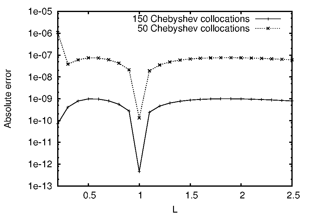
numerical singularities remains essentially unchanged. We plot in Fig. 3(A) the absolute
error between the “exact” results for the harmonic measure of the rectangle’s ends (7) and
the values obtained from solving Symm’s equations (15).
Recall that from the latter solutions we use (18) to compute . We note from Fig. 3(A)
that even for a modest number of collocations the absolute error in decreases very rapidly for a range of side lengths ; Symm’s
equations indeed give highly precise conformal maps for the rectangular geometries with the expenditure of little effort.
We will see that the situation for the Bunimovich stadium is very different in that the convergence is
limited even for large values, quite likely due to the smoothness of the
boundary for the stadium and the artificial introduction of singularities in the source densities
in (13).

Consider now the Bunimovich stadium for various lengths of the straight edges as shown in Fig. 1. The conformal
transformations are computed using Symm’s equations (15)
with collocation points in each arc. The harmonic
measure of the domes is extracted as was done for the rectangular geometry.
It is clear that for a given ,
we expect for the ends; the results for the harmonic measure are shown in
Fig. 3(B) for the two geometries, and this expectation is borne out.
However for
it is interesting to contrast the behaviour of the harmonic measure in the two cases i.e. the presence of a plateau in
the rectangle versus the sudden drop in stadium; the Brownian particle diffuses towards the horizontal edges in the
stadium much more rapidly than in the rectangle. It would be interesting, as future study, to analytically
corroborate this sudden drop in the harmonic measure
as a limiting case of the circle being infinitesimally deformed by horizontal straight edges, which corresponds to
for the stadium.
Now we focus on the length , which was studied in Sec. 3 with Monte Carlo and in Sec. 4.1 with
Schwarz-Christoffel transformations, in order to push the accuracy of map and simultaneously the measure . Symm’s equations were solved for a
range of collocation points from ; from the computed conformal maps for each case the estimate of is
listed in Table 3. We see that, unlike in the rectangular case, the convergence rate (here measured by
agreement between results from succeeding values) is not too rapid.
At values as small as (which takes the program a few seconds to complete), the value of agrees with the largest Monte Carlo runs (which took a few hours to complete). As the number of collocations are increased the digits that agree with the succeeding result are shown in bold in the table. From collocations up to and including , we are thus able to assert six digits for the harmonic measure
| (26) |
This exemplifies the point earlier made, as well in Ref. [8], that the convergence rate of the map obtained with
this method is of order for smooth boundaries; therefore to get an accuracy of 10 digits we expect that
about collocation points would be required.
Note also that the fifth digit from the naive quadratic extrapolation of the results from the Schwarz-Christoffel maps
in Fig. 2(B) agrees with (26). We have thus obtained a numerical conformal map of the stadium, using this
readily programmable algorithm of Hough et al. [8], to within an error of .
We are confident that the conformal map and the accuracy obtained in
(26) may be bettered by the use of other collocation schemes that treat the singularities
in the source densities individually or by a different numerical conformal mapping technique altogether. Of course, in order to merely
obtain higher precision for , one might consider using direct finite-element solvers of the Laplacian (1).
5. Conclusions
We have studied the problem of a Brownian particle in a Bunimovich stadium with Dirichlet boundary conditions.
Firstly a stochastic simulation of the process was employed. Further a conformal mapping of the region onto the unit disk was also undertaken;
this latter approach utilises a deterministic reformulation of the problem, which enables for a more precise analysis.
By conformally mapping the stadium to the unit disk, the harmonic measures of the boundary arcs are readily evaluated.
For the conformal transformations, two methods were undertaken:
Schwarz-Christoffel mapping of sided polygons in the large limit, and the solution of Symm’s integral
equations via a Chebyshev weighting of the solutions; using which we are able to achieve and digits of accuracy for the
harmonic measure, which
can certainly be improved by other collocation schemes or different numerical conformal mapping algorithms. The convergence rate of
the harmonic measure gives a gauge on the accuracy of the stadium’s conformal map: in particular, using Chebyshev weighted solutions Symm’s equations we obtained a conformal map of the stadium to within an absolute error of . Interesting
differences in the behaviour of the harmonic measure for the limit are exhibited between the rectangular and
stadium geometries, which we believe might be corroborated analytically for infinitesimally deformed circles.
Acknowledgment.
We thank H. Monien and T.A. Driscoll for helpful discussions and correspondence.
References
- [1] A. A. Belavin and A. M. Polyakov and A. B. Zamolodchikov, Infinite conformal symmetry in two-dimensional quantum field theory, Nuclear Physics B, Vol. 241 (1984), No. 2, 333 – 380.
- [2] F. Bornemann and D. Laurie and S. Wagon and J. Waldvogel, The SIAM 100-Digit challenge: a study in high-accuracy numerical computing, Society for Industrial and Applied Mathematics, Philadelphia, 2004.
- [3]
T.A. Driscoll,
Schwarz-Christoffel toolbox for MATLAB,
http://www.math.udel.edu/˜driscoll/SC/ - [4] T.A. Driscoll and L.N. Trefethen, Schwarz-Christoffel Mapping, Cambridge Monographs on Applied and Computational Mathematics, 8. Cambridge University Press, 2002.
- [5] M. Galassi et al., GNU Scientific Library Reference Manual, 3rd Ed., ISBN 0954612078.
- [6] M. A. Gutzwiller, Chaos in Classical and Quantum Mechanics, Interdisciplinary Applied Mathematics. Springer Verlag, New York Inc., 1990.
- [7] P. Henrici, Applied and computational complex analysis. Vol. 1, Power Series, Integration, Conformal Mapping, Location of Zeros. Pure and Applied Mathematics (New York). A Wiley-Interscience Publication. John Wiley & Sons, Inc., New York, 1986.
- [8] D .M. Hough and J. Levesley and S. N. Chandler-White, Numerical conformal mapping via Chebyshev weighted solutions of Symm’s integral equation, Journal of Computational and Applied Mathematics, Vol. 46 (1993), 29-48.
- [9] R.M. Porter, History and Recent Developments in Techniques for Numerical Conformal Mapping, Quasiconformal Mappings and their Applications (ed. by S. Ponnusamy, T. Sugawa and M. Vuorinen), Narosa Publishing House Pvt. Ltd., New Delhi, India (2007), 207–238.
- [10] A. P. Prudnikov and Yu. A. Brychkov and O. I. Marichev and N. M. Queen (Translator), Integrals and Series: Elementary Functions, CRC, 1 Edition, 1998.
- [11] R. Schinzinger and P.A.A. Laura, Conformal mapping: methods and applications, Revised edition of the 1991 original. Dover Publications, Inc., Mineola, NY, 2003.
- [12] P. Sekhar Burada and Peter Hänggi and Fabio Marcheson and Gerhard Schmid and Peter Talkner, Diffusion in confined geometries, ChemPhysChem, Vol. 10, (2009), No. 2, 45-54.
- [13] G. Symm, An Integral Equation Method in Conformal Mapping, Numerische Mathematik, Vol. 9 (1966), 250-258.