The curves not carriedThanks: This work is in the public domain.Thanks: The first author was supported by a Global Research Fellowship from the Institute of Advanced Study at the University of Warwick.
Abstract.
Suppose is a train track on a surface . Let be the set of isotopy classes of simple closed curves carried by . Masur and Minsky [2004] prove that is quasi-convex inside the curve complex . We prove that the complement, , is quasi-convex.
1. Introduction
The curve complex , of a surface , is deeply important in low-dimensional topology. One foundational result, due to Masur and Minsky, states that is Gromov hyperbolic [3, Theorem 1.1].
Suppose is a train track on . The set consists of all curves carried by : we write this as . Another striking result of Masur and Minsky is that is quasi-convex in . This follows from hyperbolicity and their result that splitting sequences of train tracks give rise to quasi-convex subsets in [4, Theorem 1.3].
We prove a complementary result.
.
Suppose is a train track. Then the curves not carried by form a quasi-convex subset of .
This supports the intuition that, for a maximal birecurrent track , the carried set is like a half-space in a hyperbolic space.
When is the four-holed sphere or once-holed torus the proof is an exercise in understanding how sits inside the Farey graph. In what follows we suppose that is a connected, compact, oriented surface with , and not a four-holed sphere. Here is a rough sketch of the proof of Theorem 3.1. Suppose and are simple closed curves, not carried by . Let be a geodesic in . Suppose and are the first and last curves of carried by . Fix splitting sequences from to and , respectively. For each splitting sequence, the vertex sets form a –quasi-convex subset inside . Since is Gromov hyperbolic, the geodesic segment is –close to the union of vertex sets. Proposition 6.1 completes the proof by showing each vertex cycle, along each splitting sequence, is uniformly close to a non-carried curve.
Before stating Proposition 6.1 we recall a few definitions. A train track is large if all components of are disks or peripheral annuli. A track is maximal if it is not a proper subtrack of any other track. The support, , of a carried curve is the union of the branches of along which runs.
.
Suppose is a train track and is a carried curve. Suppose is large, but not maximal. Then there is an essential, non-peripheral curve so that and any curve isotopic to is not carried by .
The idea behind Proposition 6.1 is as follows. Since is large all components of are disks or peripheral annuli. Since is not maximal there is a component which is not an ideal triangle or a once-holed ideal monogon. Hence, there is a diagonal of that is not carried by . We then extend , in a purely local fashion, to a simple closed curve . By construction is in efficient position with respect to and meets at most once. Finally, we appeal to Criteria 4.2 or 4.4 to show that is not isotopic to a carried curve.
2. Background
We review the basic definitions needed for the rest of the paper. Throughout we suppose is a compact, connected, smooth, oriented surface.
2.1. Corners and index
Suppose is a subsurface with piecewise smooth boundary. The non-smooth points of are the corners of . We require that the exterior angle at each corner be either or , giving inward and outward corners. Let count the inward and outward corners of , respectively. The index of is
For example, if is a rectangle then its index is zero. In general, if is a properly embedded, separating arc, avoiding the corners of , and orthogonal to , and if and are the closures of the components of , then we have .
2.2. The curve complex
Define to be the geometric intersection number between a pair of simple closed curves. The complex of curves is, for us, the following graph. Vertices are essential, non-peripheral isotopy classes of simple closed curves. Edges are pairs of distinct vertices and where . When (and is not the four-holed sphere) it is an exercise to show that is connected. We may equip with the usual edge metric, denoted . Here is a foundational result due to Masur and Minsky.
Theorem 2.3.
[3, Theorem 1.1] The curve complex is Gromov hyperbolic.
2.4. Train tracks
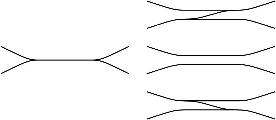
A pre-track is a non-empty finite embedded graph with various properties as follows. The vertices (called switches) are all of valence three. The edges (called branches) are smoothly embedded. Any point lying in the interior of a branch divides into a pair of half-branches. At a switch , we may orient the three incident half-branches , , and away from . After renaming the branches, if necessary, their tangents satisfy . We say is a large half-branch and and are small. This finishes the definition of a pre-track. See Figures 2.5 and 2.6 for various local pictures of a pre-track.
A branch is either small, mixed, or large as it contains zero, one, or two large half-branches. We may split a pre-track along a large branch, as shown in Figure 2.5, to obtain a new track . Conversely, we fold to obtain . If a branch is mixed then we may shift along it to obtain , as shown in Figure 2.6. Note shifting is symmetric; if is a shift of then is a shift of .
Suppose is a pre-track. We define , a tie neighborhood of as follows. For every branch we have a rectangle . For all we call a tie. The two ties of are the vertical boundary of . The boundaries of all of the ties form the horizontal boundary of . Any tie , meeting the interior of , cuts into a pair of half-rectangles. The points are the corners of ; all four are outward corners.

We embed all of the rectangles into as follows. Suppose (large) and and (small) are the half-branches incident to the switch . The vertical boundary of (respectively ) is glued to the upper (lower) third of the vertical boundary of . See Figure 2.7. The resulting tie neighborhood has horizontal boundary . The vertical boundary of is the closure of . Again is the set of corners of ; all of these are inward corners. We use to denote the interior of . We may now give our definition of a train track.
Definition 2.8.
Suppose is a pre-track and is a tie neighborhood. We say is a train track if every component of has negative index.
A track is large if every component of is either a disk or a peripheral annulus. A track is maximal if every component of is either a hexagon or a once-holed bigon.
2.9. Carried curves and transverse measures
Suppose is a simple closed curve. If and is transverse to the ties of then we say is carried by . We write this as . It is an exercise to show that if is carried then is essential and non-peripheral. We define . Note that is non-empty.
Let be the set of branches of . Fix a switch and suppose that the half-branches , , and are adjacent to , with being large. A function satisfies the switch equality at if
We call a transverse measure if satisfies all switch equalities. For example, any carried curve gives an integral transverse measure . This permits us to define , the support of in : a branch lies in if .
Here is a “basic observation” from [3, page 117].
Lemma 2.10.
Suppose is a maximal train track and suppose has full support: . Suppose is an essential, non-peripheral curve with . Then is also carried by . ∎
Since the switch equalities are homogeneous the set of solutions is a rational cone. We projectivize to obtain , a non-empty convex polytope. All vertices of arise from carried curves; we call such curves vertex cycles for . Thus the set of vertex cycles is naturally a subset of . Deduce if is a shift of then .
Lemma 2.12.
A carried curve is a vertex cycle if and only if is either a simple close curve or a barbell (see Figure 2.11).
Proof.
The forward direction is given by Proposition 3.11.3(3) of [5]. The backward direction is an exercise in the definitions. ∎
The usual upper bound on distance in , coming from geometric intersection number [6, Lemma 1.21], gives the following.
Lemma 2.13.
For any surface there is a constant with the following property. Suppose is a track. Suppose is a split, shift, or subtrack of . Then the diameter of inside of is at most . ∎
2.14. Quasi-convexity
A subset is –quasi-convex if for every and in , any geodesic lies within a –neighborhood of . Recall if and are –quasi-convex sets in , and if is non-empty, then the union is –quasi-convex. We now have a more difficult result.
Theorem 2.15.
[4, Theorem 1.3] For any surface there is a constant with the following property. Suppose that is sequence where is a split, shift, or subtrack . Then the set is –quasi-convex in . ∎
Remark 2.16.
In the first statement of their Theorem 1.3 [4, page 310] Masur and Minsky assume their tracks are large and recurrent. However, as they remark after their Lemma 3.1, largeness is not necessary. Also, it is an exercise to eliminate the hypothesis of recurrence, say by using Lemma 2.13 and the subtracks (for any fixed curve ).
A more subtle point is that their Lemmas 3.2, 3.3, and 3.4 use the train-track machinery of another of their papers [3]. Transverse recurrence is used in an essential way in the second paragraph of the proof of Lemma 4.5 of that earlier paper. However the crucial “nesting lemma” [4, Lemma 3.4] can be proved without transverse recurrence. This is done in Lemma 3.2 of [1].
Thus, as stated above, Theorem 2.15 does not require any hypothesis of largeness, recurrence, or transverse recurrence.
3. Proof of the main theorem
We now have enough tools in place to see how Proposition 6.1 implies our main result.
Theorem 3.1.
Suppose is a train track. The curves not carried by form a quasi-convex subset of .
Proof.
We may assume , and that is not a four-holed sphere. Suppose are not carried by . Fix a geodesic in . If is disjoint from there is nothing to prove.
So, instead, suppose and are the first and last curves, along , carried by . Let be the predecessor of in and let be the successor of . Thus, and are not carried by . The contrapositive of Lemma 2.10 now implies that the tracks and are not maximal.
For the moment, we fix our attention on . We choose a splitting and shifting sequence with the following properties:
- •
,
- •
for all , the curve is carried by , and
- •
is a simple closed curve.
We find a similar sequence for .
Let be the vertices of the splitting sequence ; define similarly. The hyperbolicity of (Theorem 2.3) and the quasi-convexity of vertex sets (Theorem 2.15) imply the geodesic lies within a –neighborhood of . To finish the proof we must show that every vertex of (and of ) is close to a non-carried curve of .
Using Lemma 2.12 twice we may pick vertex cycles so that:
- •
and
- •
.
Define . By construction . If we fold backwards along the sequence then, the former track yields while the latter yields . We deduce . Recall that is not maximal. Thus none of the are maximal.
Let . Fix any curve disjoint from . Using we deduce , for any .
If then Lemma 2.13 implies the set lies within a –neighborhood of , and we are done.
So we may assume that . In this case Lemma 2.13 implies the set lies within a –neighborhood of . Recall and is assumed to be a large, yet not maximal, subtrack of . Thus we may apply Proposition 6.1 to obtain a curve so that:
- •
and
- •
.
Applying Lemma 2.13 we deduce, whenever , that lies within a –neighborhood of .
The same argument applies to the splitting sequence from to . This completes the proof of the theorem. ∎
4. Efficient position
In order to prove Proposition 6.1, we here give criteria to show that a curve cannot be carried by a given track . We state these in terms of efficient position, defined previously in [2, Definition 2.3]. See also [7, Definition 3.2].
Suppose is a train track and is a tie neighborhood. A simple arc , properly embedded in , is a carried arc if it is transverse to the ties and disjoint from .
Definition 4.1.
Suppose is a properly embedded arc or curve which is transverse to and disjoint from , the corners of . Then is in efficient position with respect to , written , if
- •
every component of is carried or is a tie and
- •
every component of has negative index or is a rectangle.
Here is a shorthand for , where the ties of are either subties of, or orthogonal to, ties of . An index argument proves if then is essential and non-peripheral. See [2, Lemma 2.5].
Criterion 4.2.
Suppose is a curve. Orient . Suppose there are regions and of and a component with the following properties.
- •
and lie immediately to the left and right, respectively, of and
- •
and have negative index.
Then any curve isotopic to is not carried by .
2pt
\pinlabel at 107 107
\pinlabel at 163 163
\pinlabel [tr] at 166 110
\endlabellist \labellist\hair
2pt
\pinlabel at 32 119
\pinlabel at 94 28
\pinlabel [l] at 65 73
\endlabellist
\labellist\hair
2pt
\pinlabel at 32 119
\pinlabel at 94 28
\pinlabel [l] at 65 73
\endlabellist
Proof.
Suppose, for a contradiction, that is isotopic to . We now induct on the intersection number .
In the base case and are disjoint; thus and cobound an annulus . Since and are in efficient position with respect to , the intersection is a union of rectangles, so has index zero. However, one of or lies inside of . This contradicts the additivity of index.
In the induction step, and cobound a bigon . Since is carried, the two corners and of lie inside of . Let be the component of that contains . We call a carried or dual corner as is a carried arc or a tie. We use the same terminology for .
If is a carried corner then move along a small amount, let be the resulting tie, and use to cut a triangle (containing ) off of to obtain . Do the same at to obtain . Now, if both and are dual corners then is a bigon. If exactly one of or is a dual corner then is a triangle. In either of these cases is positive, contradicting the assumption that is in efficient position.
So suppose both and are carried corners of ; thus is a rectangle. Thus has index zero. Recall that is a subarc of meeting both and . Since neither or lie in deduce that is disjoint from . We now define and , the two sides of . We define to be the curve obtained from by isotoping across , slightly past . So is isotopic to , is in efficient position with respect to , has two fewer points of intersection with , and contains . Thus is adjacent to two regions and of of negative index, as desired. This completes the induction step and thus the proof of the criterion. ∎
Criterion 4.2 is not general enough for our purposes. We also need a criterion that covers a situation where the regions and are not immediately adjacent.
Criterion 4.4.
Suppose is a curve. Orient . Suppose there are regions and of and a tie with the following properties.
- •
and lie to the left and right, respectively, of ,
- •
the two points of are corners of and , and
- •
and have negative index.
Then any curve isotopic to is not carried by . ∎
5. Efficient and crossing diagonals
The next tool needed to prove Proposition 6.1 is the existence of crossing diagonals: efficient arcs that cannot isotoped to be carried.
Let be a train track. Suppose is a subtrack. We take to be a tie sub-neighborhood, as follows.
- •
Every tie of is a subarc of a tie of .
- •
The horizontal boundary is
- –
disjoint from and
- –
transverse to the ties of .
- –
- •
Every component of contains a component of .
Now suppose that is a component of . We define . We say that a properly embedded arc is a diagonal of if
- •
lies in , missing the corners,
- •
is orthogonal to , and
- •
all components of have negative index.
A diagonal is efficient if it satisfies Definition 4.1 with respect to . An efficient diagonal is short if one component of is a hexagon. The hexagon meets three (or two) components of and properly contains one of them, say . In this situation we say cuts off of . In the simplest example a short diagonal is carried by .
We say an efficient diagonal is a crossing diagonal if there is
- •
a subarc (or ) and
- •
regions and of
satisfying the hypotheses of Criterion 4.2 or Criterion 4.4. Deduce, if is a curve containing a crossing diagonal , that any curve isotopic to is not carried by .
Lemma 5.1.
Suppose is a large subtrack. Let be a component of that is not a hexagon or a once-holed bigon. Then for any component there is a short diagonal that cuts off of .
Furthermore is properly isotopic, relative to the corners of , to a carried or a crossing diagonal.
Proof. The orientation of induces an oriention on and thus of the boundary of . Let and be the components of immediately before and after . (Note that we may have . In this case is a once-holed rectangle.) Let and be the components of immediately before and after .
Let be the union of the ties of meeting . As usual, is a union of rectangles. (See Figure 5.2 for one possibility for .) Let be a tie of , meeting the interior of . Suppose that contains a component of . Thus locally divides into a pair of half-rectangles, one large and one small. When the small half-rectangle is closer to than it is to (along ), we say faces . Among the ties of facing , let be the one closest to . (If no tie faces we take .)
2pt
\pinlabel [r] at 1 47
\pinlabel [l] at 399 47
\pinlabel [l] at 218 63
\pinlabel [bl] at 385 83
\endlabellist
With in hand, let be the closure of the component of that meets . We define and in the same way, with respect to .
2pt
\pinlabel [l] at 136 92
\endlabellist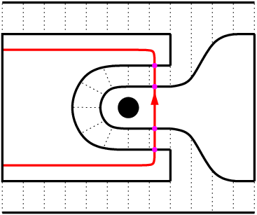
Consider the set . Let be a small regular neighborhood of , taken in , and set ; see Figure 5.2. Note that cuts off of . Orient so that is to the right of .
We now prove that is in efficient position, after an arbitrarily small isotopy. The subarc of between and is carried; the same holds for the subarc between and . (If then we take and similarly for .) All components of , other than and , are ties.
Consider . If is connected, then cuts a hexagon off of . By additivity of index the region adjacent to has index at most zero. If has index zero, it is a rectangle; we deduce that is isotopic to a carried diagonal. If has negative index then is a crossing diagonal, according to Criterion 4.2.
Suppose is not connected. We deduce that the first and last components of cut pentagons off of ; all other components cut off rectangles. When then every region of contains at most one component of . In this case an index argument proves that is a crossing diagonal, according to Criterion 4.2. If then is a once-holed rectangle as shown in Figure 5.3. In this case is a crossing diagonal, according to Criterion 4.4. ∎
Lemma 5.4.
Suppose is a large subtrack. Let be a component of that is not a hexagon or a once-holed bigon. Then has a short crossing diagonal.
Proof.
Since is large, is a disk or a peripheral annulus. Set . According to Lemma 5.1, for every component there is a short diagonal cutting off of . Let be the hexagon to the right of . Also every is a carried or a crossing diagonal.
Suppose for a contradiction that is carried, for each . Thus is again a hexagon. If is another component of then and are disjoint. Since index is additive, we find . This inequality is strict when is a peripheral annulus; this is because the component of meeting must also have negative index.
On the other hand, if is a disk then ; if is an annulus then . In either case we have a contradiction. ∎
6. Closing up the diagonal
After introducing the necessary terminology, we give the proof of Proposition 6.1.
Suppose is a track, and is a tie neighborhood. Suppose that is a tie, containing a component . Let be the large half-rectangle adjacent to . For any unit vector based at we say is vertical if it is tangent to , is large if it points into , and is small otherwise. Suppose is a carried curve. A point is innermost on if there is a component so that the closure of meets both and .
Fix an oriented curve . For any , we write for the unit tangent vector to at . If then we take to be (the closure of) the component of where points into . Note that . Also, we take to be equipped with the opposite orientation. We make similar definitions when is a arc.
Proposition 6.1.
Suppose is a train track and is a carried curve. Suppose is large, but not maximal. Then there is a curve so that and any curve isotopic to is not carried by .
Proof.
Set . Fix a component of that is not a hexagon or a once-holed bigon. By Lemma 5.4 there is a short crossing diagonal . Recall that cuts a hexagon off of ; also, is oriented so that is to the right of . The hexagon meets three components . The component is completely contained in ; also, we may have . Let and be the initial and terminal points of , respectively. Thus and ; also is small and is large. (Equivalently, points into while points out of .)
Let and be the ties of containing and . Rotate by , counterclockwise, to get an orientation of . We do the same for .
Since , there are pairs of innermost points and . We choose names so that is the order of the points along and so that is the order along . Now orient so that is small.
2pt
\pinlabel [b] at 137 59
\pinlabel [r] at 36 57
\pinlabel [l] at 238 57
\pinlabel [br] at 36 31
\pinlabel [br] at 36 85
\pinlabel [bl] at 237 31
\pinlabel [tl] at 237 91
\endlabellist
We divide the proof into two main cases: one of , , is large, or all three vectors are small. In all cases and subcases our goal is to construct a curve which contains and is, after an arbitrarily small isotopy, in efficient position with respect to . Since contains one of Criterion 4.2 or Criterion 4.4 applies: any curve isotopic to is not carried by .
6.3. A tangent vector to at , , or is large.
This case breaks into subcases depending on whether or not . Suppose first that .
If is large, then consider the arcs , , and . The curve
has the desired properties and satisfies .
If is large, then consider the arcs , , and . Then
has because crosses, once, from the right side to the left side of .
Suppose now that and are small but is large. Consider the arcs , , and . Then
has .
We now turn to the subcase where and is large. In this case , , and the points appear, in that order, along . Consider the arcs and and . Then
has .
6.4. The tangent vectors to at , , and are small.
Let be the biggest rectangle, with embedded interior, where
- •
both components of are subarcs of ties,
- •
is a component of , and
- •
.
Since the interior of is embedded, the vertical arc contains a unique component ; also, the component is not equal to . Pick a point in the interior of . Let be a carried arc starting at , ending at , and oriented away from .
Let be the tie in containing . We orient by rotating by , counterclockwise. Let and be the innermost points of . Note that and are both large. Thus . We have already seen that .
Let be the component of that contains . The orientation on restricts to , which in turn induces an orientation on . Let be the component of immediately before .
If then is a once-holed bigon, contradicting the fact that and are both large.
If then is the hexagon to the right of . Thus . In this case there is a curve so that
- •
is a properly embedded arc with endpoints and and
- •
is a component of .
Thus is isotopic to (the right side of) . Now, if then also meets the region , near . Thus is not contained in , a contradiction. If then is a once-holed rectangle. In this case , together with a pair of rectangles, is all of . Thus is a once-holed torus, contradicting our standing assumption that .
If then . We deduce that is not a once-holed rectangle; so . Also, the left side of is contained in . However the left side of meets the hexagon , near the point , giving a contradiction.
To recap: the arc enters at . The region is not a once-holed bigon; also . The component coming before is not contained in .
Let be the tie of containing . We orient using the orientation of . Let and be the two innermost points of , where comes before along . Since is large, the vector is small.
We now have a final pair of subcases. Either is large, or it is small.
6.5. The tangent vector to at is large.
Consider the arcs , , , , and . Then
has . (Note that after an arbitrarily small isotopy the arc becomes carried.)
6.6. The tangent vector to at is small.
In this case we consider the component of immediately before . Recall that . Now, if is the left component of then being small implies is large, contrary to assumption. If is the left component of then is contained in , a contradicton.
As usual, let be the tie in containing . Since is not contained in or there are a pair of innermost points and along . Applying Lemma 5.1 there is a short diagonal in that
- •
connects to a point and
- •
cuts off of .
Note that is to the left of .
We give the orientation coming from ; this agrees with the orientation given by rotating by angle , counterclockwise. We choose names so the points come in that order along .
Consider the arcs , , and . Then
has because crosses, once, from the right side to the left side of . This is the final case, and completes the proof. ∎
2pt \pinlabel [tl] at 4 92 \pinlabel [br] at 360 24 \pinlabel [r] at 31 59 \pinlabel [l] at 111 76 \pinlabel [Bl] at 111 44 \pinlabel [l] at 333 59 \pinlabel [Br] at 254 80 \pinlabel [r] at 254 40 \pinlabel [br] at 179 58 \pinlabel [b] at 110 115 \pinlabel [t] at 110 -1 \pinlabel [t] at 254 2 \pinlabel [b] at 254 114 \endlabellist

References
- [1] Vaibhav Gadre and Chia-Yen Tsai. Minimal pseudo-Anosov translation lengths on the complex of curves. Geom. Topol., 15(3):1297–1312, 2011, arXiv:1101.2692.
- [2] Howard Masur, Lee Mosher, and Saul Schleimer. On train-track splitting sequences. Duke Math. J., 161(9):1613–1656, 2012, arXiv:1004.4564v1.
- [3] Howard A. Masur and Yair N. Minsky. Geometry of the complex of curves. I. Hyperbolicity. Invent. Math., 138(1):103–149, 1999, arXiv:math/9804098v2.
- [4] Howard A. Masur and Yair N. Minsky. Quasiconvexity in the curve complex. In In the tradition of Ahlfors and Bers, III, volume 355 of Contemp. Math., pages 309–320. Amer. Math. Soc., Providence, RI, 2004, arXiv:math/0307083v1.
- [5]
Lee Mosher.
Train track expansions of measured foliations.
2003.
http://math.newark.rutgers.edu/mosher/. - [6]
Saul Schleimer.
Notes on the complex of curves.
http://www.warwick.ac.uk/masgar/Maths/notes.pdf. - [7] Itaru Takarajima. A combinatorial representation of curves using train tracks. Topology Appl., 106(2):169–198, 2000.