Benchmark stars for Gaia.
Fundamental properties of the
Population II star HD 140283 from interferometric,
spectroscopic, and photometric dataThanks: Based on observations with the VEGA/CHARA spectrointerferometer.Thanks: Based on NARVAL and HARPS data obtained within the Gaia DPAC (Data Processing and Analysis Consortium) and coordinated by the GBOG (Ground-Based Observations for Gaia) working group, and on data retrieved from the ESO-ADP database.Thanks: Table 12 only available in full in electronic form at the CDS via anonymous ftp to cdsarc.u-strasbg.fr (130.79.128.5) or via http://cdsweb.u-strasbg.fr/cgi-bin/qcat?J/A+A/
Abstract
Metal-poor halo stars are important astrophysical laboratories that allow us to unravel details about many aspects of astrophysics, including the chemical conditions at the formation of our Galaxy, understanding the processes of diffusion in stellar interiors, and determining precise effective temperatures and calibration of colour-effective temperature relations. To address any of these issues the fundamental properties of the stars must first be determined. HD 140283 is the closest and brightest metal-poor Population II halo star (distance = 58 pc and ), an ideal target that allows us to approach these questions, and one of a list of 34 benchmark stars defined for Gaia astrophysical parameter calibration. In the framework of characterizing these benchmark stars, we determined the fundamental properties of HD 140283 (radius, mass, age, and effective temperature) by obtaining new interferometric and spectroscopic measurements and combining them with photometry from the literature. The interferometric measurements were obtained using the visible interferometer VEGA on the CHARA array and we determined a 1D limb-darkened angular diameter of = 0.353 0.013 milliarcseconds. Using photometry from the literature we derived the bolometric flux in two ways: a zero reddening solution (AV = 0.0 mag) of of 3.890 0.066 x 10⁻⁸ erg s-1 cm-2, and a maximum of AV = 0.1 mag solution of 4.220 0.067 x 10⁻⁸ erg s-1 cm-2. The interferometric is thus between 5534 103 K and 5647 105 K and its radius is = 2.21 0.08 R⊙. Spectroscopic measurements of HD 140283 were obtained using HARPS, NARVAL, and UVES and a 1D LTE analysis of H line wings yielded spec = 5626 75 K. Using fine-tuned stellar models including diffusion of elements we then determined the mass and age of HD 140283. Once the metallicity has been fixed, the age of the star depends on , initial helium abundance , and mixing-length parameter , only two of which are independent. We derive simple equations to estimate one from the other two. We need to adjust to much lower values than the solar one () in order to fit the observations, and if AV = 0.0 mag then . We give an equation to estimate from , (), and AV. Establishing a reference and adopting = 0.245 we derive a mass and age of HD 140283: = 0.780 0.010 M⊙ and = 13.7 0.7 Gyr (AV = 0.0 mag), or = 0.805 0.010 M⊙ and = 12.2 0.6 Gyr (AV = 0.1 mag). Our stellar models yield an initial (interior) metal-hydrogen mass fraction of and = 3.65 0.03. Theoretical advances allowing us to impose the mixing-length parameter would greatly improve the redundancy between , and age, while from an observational point of view, accurate determinations of extinction along with asteroseismic observations would provide critical information allowing us to overcome the current limitations in our results.
Key Words.
Stars: fundamental properties — Stars: individual HD 140283 — Stars: low-mass — Stars: Population II — Galaxy: halo — Techniques: interferometry1 Introduction
The determination of accurate and precise stellar properties (radius , effective temperature , age, , …) of metal-poor halo stars is a primary requirement for addressing many astrophysical questions from stellar to galactic physics. For example, improving our knowledge of stellar interior processes (diffusion and Li depletion e.g. Bonifacio & Molaro 1998; Lebreton 2000; Charbonnel & Primas 2005; Korn et al. 2007; Meléndez et al. 2010) and evolution models has important consequences for determining the precise ages of stars and clusters (e.g. Grundahl et al. 2000), and thus for determining the age, and formation history of our Galaxy, e.g. Yamada et al. (2013); Haywood et al. (2013).
The effective temperature is a particularly important fundamental quantity to determine. This has consequences for deriving masses and ages of stars through a HR diagram analysis, and determinations of absolute abundances require accurate preferably a priori along with accurate knowledge of surface gravities . However, determining is difficult, and calibrating this scale has been the subject of many recent important studies, e.g. Casagrande et al. (2010). While much progress has been made, the temperature scales still remain to be fully validated at the low-metallicity and high-metallicity regimes. This is particularly important in the context of large-scale photometric surveys where many low metallicity stars are observed and provide important tests of stellar structure conditions quite different to those of our Sun, and hence of Galactic structure and evolution.
With recent developments from asteroseismology, in particular for cool FGK stars using the space-based telescopes CoRoT and Kepler, determinations of precise fundamental properties for large samples of stars is possible, with direct consequences for galactic astrophysics. Mean densities can be determined with precisions of the order of % and in combination with other data, masses and ages reach precisions of 5% and % (Metcalfe et al. 2009; Silva Aguirre et al. 2013; Lebreton & Goupil 2014; Metcalfe et al. 2014). Asteroseismic scaling relations which predict masses, radii and surface gravity from simple relations using global seismic quantities (Brown & Gilliland 1994; Kjeldsen & Bedding 1995) have a huge potential for stellar population studies and galacto-archaeology. However, while these relations have been validated in some regimes such as main sequence stars (Metcalfe et al. 2014; Huber et al. 2012; Creevey et al. 2013), they have yet to be validated in the metal-poor regime (e.g. Epstein et al. 2014). Independent determinations of radii and masses of these stars provide valuable tests of the widely-applicable relations.
Combining high precision distances that Gaia11 1 http://sci.esa.int/gaia/ will yield with robust determinations of predicted angular diameters from temperature-colour relations (e.g. Kervella et al. 2004; Boyajian et al. 2014) yields one of the most constraining observables for stellar models: the radius. These various arguments clearly demonstrate the need for very thorough studies of the most fundamental properties of nearby bright stars.
The Gaia mission (e.g. Perryman 2005) was successfully launched at the end of 2013. In addition to distances and kinematic information, it will also deliver stellar properties for one billion objects (Bailer-Jones et al. 2013). In preparation for this mission a set of priority bright stars has been defined22 2 http://www.astro.uu.se/~ulrike/GaiaSAM/. Extensive observations and analyses have been made on these benchmark stars, with the aim of using them to define (and refine) the stellar models that will be used for characterizing the one billion objects Gaia will observe. One of these benchmark stars is HD 140283 and a thorough analysis of its fundamental properties is timely.
HD 140283 (BD-10~4149, HIP~76976, = 15h 43m 03s, , ) is a metal-poor Galactic Halo (Population II) star. It is bright ( mag) and nearby (58 pc) and thus a benchmark for stellar and galactic astrophysics. HD 140283 has been the subject of numerous studies, especially in more recent years where more sophisticated stellar atmosphere models have been used to determine accurate metallicities and abundances (e.g. Charbonnel & Primas 2005) and to study neutron-capture elements to understand better heavy element nucleosynthesis (Siqueira Mello et al. 2012; Gallagher et al. 2010; Collet et al. 2009). Concerning the fundamental properties of this star, Bond et al. (2013) published a refined parallax = 17.15 +- 0.14 mas, an uncertainty one fifth of that determined by the Hipparcos satellite (van Leeuwen 2007, 17.16 0.68 mas), and assuming zero reddening determined an age of 14.5 Gyr. More recently, VandenBerg et al. (2014) determined an age for HD 140283 of 14.27 Gyr. These ages are slightly larger than the adopted age of the Universe (13.77 Gyr, Bennett et al. 2013) but within their quoted error bars. The new better precision in the parallax from Bond et al. (2013) reduces the derived uncertainty in the radius (this work) by a factor of 30% and leaves the radius uncertainty dominated almost entirely by its angular diameter.
The objective of this work is to determine the radius, mass, age, effective temperature, luminosity, and surface gravity of HD 140283. We present the very first interferometric measurements of this object obtained with the visible interferometer VEGA (Mourard et al. 2011) mounted on the CHARA array (ten Brummelaar et al. 2005) in California, USA (Sect. 2). Our observations also show the capabilities of this instrument to operate at a magnitude of V=7.2 (without adaptive optics) and at very high angular resolution (0.35 milliarcseconds, mas), one of the smallest angular diameters to be measured. We combine these interferometric data with multi-band photometry (Sect. 3), to derive the fundamental properties of HD 140283 (Sect. 4). We then analyse high-resolution spectra (Sect. 5) to determine its while imposing from our analysis. In Sect. 7 we use the stellar evolution code CESAM to interpret our observations along with literature data (Sect. 6) to infer the stellar model properties (mass, age, initial abundance). We discuss the limitations in our observations, models, and analysis (Sect. 8) and we conclude by listing the next important observational and theoretical steps for overcoming these limitations.
2 CHARA/VEGA interferometric observations and the angular diameter of HD 140283
Interferometric observations of HD 140283 were performed on four nights during 2012 and 2014 using the VEGA instrument on the CHARA Array and the instrument CLIMB (Sturmann et al. 2010) for 3T group delay tracking. The telescopes E1, W1, and W2 were used for all of the observations, providing baselines of roughly 100 m, 221 m, and 313 m. Table 1 summarizes these observations. In this table, the sequence refers to the way the observations were made where a typical calibrated point consists of observations of a calibrator star, the target star, and again a calibrator star. We obtained a total of five calibrated points. The extracted (squared visibility) measurements for the target star alone are the instrumental and these need to be calibrated by stars with known diameters. We used a total of three different calibrator stars whose predicted uniform disk angular diameters in the R band are given in the caption of the table. These were estimated using surface brightness relations for and as provided by the SearchCal tool of JMMC (Bonneau et al. 2006). SearchCal also provides the limb-darkened-to-uniform-disk converted angular diameters, and the latter are used for calibrating the data. The average seeing during the full observation sequence is given in the following column by the Fried parameter r0. This parameter gives the typical length scale over which the atmosphere can be considered uniform. Perfect conditions can have r0 of the order of 20 cm, while poor conditions have r0 of approximately 5cm. Our observations were conducted in poor to average seeing conditions (low altitude and non-optimal observing season), resulting in larger errors on the data and the loss of some points (see below).
| Date | Sequence | r0 | Bands processed/ | No. of potential | Useful |
|---|---|---|---|---|---|
| dd-mm-yr | (cm) | width (nm) | points | ||
| 2012-April-18 | C1-T-C1 | 5-8 | 3/10 | 9 | 1 |
| 2012-May-21 | C2-T-C1 | 7-10 | 4/10 | 12 | 12 |
| 2014-May-03 | C2-T-C2-T-C2 | 8-10 | 1/20 | 6 | 4 |
| 2014-May-04 | C2-T-C3-T-C1 | 7-10 | 1/20 | 6 | 2 |
.
2.1 Extraction of squared visibilities
We used the standard V2 reduction procedure of the VEGA instrument as described in Mourard et al. (2011) to process the data. Depending on the quality of the data, the observations were processed in a number of bands of different width. The wavelength coverage of the VEGA R/I band is nm. For the observations from 2012 we processed the data in four spectral bands of 10nm each, centred on 705nm, 715m, 725nm, and 735nm. Because of the lower signal-to-noise ratio (S/N), for the 2014 observations we processed the data in one band of 20nm centred on 710nm44 4 Each observation of a star (either calibrator or target) consists of a total of N blocks of 1000 exposures. The calibrator observations consist of 20 blocks, while the target observations from 2012 consist of 60 blocks and those of 2014 consist of 30 blocks.. Table 1 summarizes this information under the column heading Band processed/width. The number of potential points depends on the number of bands processed, the number of calibrated points, and the number of telescopes pairs (in this case three) for each observation sequence. In some cases (variable seeing, poor S/N on target or calibrator) the visibility calibration fails. Thus, in the final column of Table 1 we give the number of points that were successfully extracted from each observation sequence, resulting in a total of 19 usable points. Some of the data were processed independently and the resulting varied only in the third decimal place with no consequence for the angular diameter derivation. The calibrated visibilities have an associated intrinsic statistical error and an external error coming from the uncertainty on the angular diameter of the calibrators, and the total error is given as the quadratic sum of the two components (Mourard et al. 201255 5 https://www-n.oca.eu/vega/en/publications/spie2012vega.pdf). By observing on different nights and by using different calibrators we reduced the possibility of systematic errors in our analysis. Table 2 lists the squared visibilities , along with the errors separated into the statistical and external errors , the projected baselines66 6 The projected baseline Bp depends on a number of factors including the physical distance between the telescope pair (baseline), the angles of the baseline compared to the north-east direction and the altitude of the object over the horizon, see e.g. Nardetto, N. PhD thesis, 2005, pg. 57 http://tel.archives-ouvertes.fr Bp, and the effective wavelengths of the 19 points.
| Date | Bp | ||||
|---|---|---|---|---|---|
| (dd-mm-yy) | (m) | (nm) | |||
| 2012-April-18 | 0.755 | 0.222 | 0.007 | 94.087 | 715.0 |
| 2012-May-21 | 0.790 | 0.102 | 0.006 | 93.171 | 705.0 |
| 2012-May-21 | 0.210 | 0.097 | 0.023 | 310.487 | 705.0 |
| 2012-May-21 | 0.659 | 0.158 | 0.038 | 221.555 | 705.0 |
| 2012-May-21 | 0.886 | 0.133 | 0.006 | 93.171 | 715.0 |
| 2012-May-21 | 0.213 | 0.052 | 0.023 | 310.487 | 715.0 |
| 2012-May-21 | 0.469 | 0.079 | 0.026 | 221.555 | 715.0 |
| 2012-May-21 | 1.043 | 0.157 | 0.007 | 93.171 | 725.0 |
| 2012-May-21 | 0.269 | 0.078 | 0.028 | 310.487 | 725.0 |
| 2012-May-21 | 0.311 | 0.134 | 0.017 | 221.555 | 725.0 |
| 2012-May-21 | 0.914 | 0.140 | 0.006 | 93.171 | 735.0 |
| 2012-May-21 | 0.365 | 0.062 | 0.037 | 310.487 | 735.0 |
| 2012-May-21 | 0.456 | 0.110 | 0.024 | 221.555 | 735.0 |
| 2014-May-03 | 0.541 | 0.086 | 0.042 | 221.627 | 710.0 |
| 2014-May-03 | 0.844 | 0.052 | 0.009 | 92.743 | 710.0 |
| 2014-May-03 | 0.534 | 0.145 | 0.033 | 218.142 | 710.0 |
| 2014-May-03 | 0.872 | 0.064 | 0.011 | 99.990 | 710.0 |
| 2014-May-04 | 0.852 | 0.149 | 0.054 | 96.074 | 710.0 |
| 2014-May-04 | 0.245 | 0.164 | 0.047 | 312.384 | 710.0 |
2.2 From visibilities to an angular diameter
To determine the uniform disk and 1D angular diameters, we performed non-linear least-squares fits of the squared-visibility data to visibility functions using the Levenberg-Marquardt algorithm (Press et al. 1992). Table 3 lists the uniform disk , 1D limb-darkened , and 3D limb-darkened angular diameters and uncertainties, all explained in the following paragraphs.
2.2.1 Uniform disk angular diameter
Fitting the data to a uniform disk angular diameter ignoring the external errors yields = 0.338 0.011 mas with a = 0.586. Including the external errors as gives = 0.340 0.012 mas with a = 0.529.
2.2.2 1D limb-darkened angular diameter
The 1D limb-darkened disk function is given by
| (1) |
where is the wavelength dependent limb-darkening coefficient, is the Bessel function of order , and . The value of was obtained by interpolating the linear limb-darkening coefficients from Claret et al. (2012) (‘u’ in their work) for the stellar parameters = 5500 and 5750 K, = 3.75 and [M/H] = –2.10 (see Sect. 7). We adopted the coefficients halfway between the R and I tabulated values, which correspond to the effective wavelengths of the measurements. The resulting values vary between 0.4795 and 0.4870 for the range of found in this work. Using the values of = 3.50 or [M/H] = –2.0 yields limb-darkening coefficients that vary in the third decimal place and these result in a change in 1D in the fourth decimal place.
The value of can in principle also be fitted, however, the brightness contrast is larger at the border of the projected disk of the star that corresponds to visibilities close to and just after the first zero point. Our data do not extend to the first zero point nor is the coverage at lower visibility sufficient to constrain . Just as in the case of many other studies we adopt model-dependent values.
A fit to a 1D limb-darkened disk angular diameter adopting the errors yields = 0.353 0.012 mas with . The data and the corresponding visibility curve are shown in the top panel of Fig. 1, while the residuals scaled by the individual errors on the measurements are shown in the bottom panel.
At such small angular diameters with calibrators of similar size the external error could have an important effect on our derived diameter. To show explicitly the effect of this error we performed Monte Carlo-type simulations. We simulated 10,000 sets of visibility points and using the original statistical errors as the uncertainties in the data we fitted these data to 1D limb-darkened visibility functions. A simulated set of visibility points was obtained by adding a random number drawn from a Gaussian distribution with a mean of zero and a standard deviation of 1, scaled by the external errors as follows: for each point in each set. For the 10,000 simulated sets we obtained 10,000 fitted angular diameters .


The distribution of angular diameters from the simulations is shown in Figure 2 by the inner grey distribution, where the binsize of 0.0007 mas is determined by the Freedman-Diaconis rule77 7 The width of each bin is given by , where is the number of points and is the interquartile range. The dark-shaded region corresponds to the 68% probability region (, where the subscript ‘’ refers to the uncertainty on the derived diameter as opposed to the measurement errors), and represents a total of 0.008 mas or (see Table 3). We also overplot a Gaussian function representing the fitted angular diameter and the 68% probability region corresponding to the statistical uncertainty (light grey shaded region). In this case the external errors do not contribute significantly to the total error, but if the statistical errors were much smaller then it would be of interest to reduce this external error. The uncertainty on the final adopted 1D limb-darkened diameter is obtained by adding the statistical and external error in quadrature and this yields mas (see Table 6), in agreement with the uncertainty obtained when fitting the data using the total measurement errors (). Any systematic affecting the determination of the diameter can only be evaluated by comparing this result with an independently determined angular diameter.
| 0.338 | 0.011 | 0.004 | 0.012 | 0.586 | |
| 0.353 | 0.012 | 0.004 | 0.013 | 0.581 | |
| 0.352 | 0.012 | 0.004 | 0.013 | 0.582 |
2.2.3 3D limb-darkened angular diameter
We also calculated the limb-darkened diameter considering realistic 3D simulations of surface convection. Generally (Bigot et al. 2006; Bigot et al. 2011; Chiavassa et al. 2009; Chiavassa et al. 2012), which is due to a smoother hydrodynamical temperature gradient in the surface layers compared with the hydrostatic gradient, although for non-evolved stars this difference may not be significant even in the visible wavelengths which are more sensitive to this effect. Casagrande et al. (2014) recently pointed out a very small discrepancy between their absolute scale from the infra-red flux method (IRFM) and measured angular diameters and attributed it to the fact that 1D interferometric diameters are usually quoted and not 3D ones. In most cases the precision in the measurements is not sufficient to distinguish between the two; however, their work did show an almost perfect agreement between the derived from a 3D angular diameter of the metal-poor giant HD 122563 from Creevey et al. (2012) and their IRFM value (a difference of 8 K in ). For this reason we performed a 3D analysis. The method follows that of Bigot et al. (2011) and we refer the readers to this paper for details. Briefly, the 3D limb-darkened profiles are obtained by computing the full 3D monochromatic line transfer within the wavelength range of the VEGA red camera at different inclination angles. We then averaged the monochromatic limb-darkened profiles within each bandwidth (10-20nm) around the central wavelengths. The parameters that define the 3D model of granulation were 5650 K (temporal average), logg = 3.65 and [M/H] = –2.0. By comparing the 3D limb-darkened intensity profile directly with the 1D profile using a limb-darkening law and the adopted 1D coefficients, we find an average difference of 1% between the two profiles for over 99% of the linear diameter of the star. A fit to the data yields mas very close to the 1D profile. The difference between the 3D and 1D is negligible for HD 140283 since its limb darkening is very weak because of the lack of metals in its atmosphere. For the rest of the work, we adopt the 1D value to derive the stellar parameters (see Table 6).
3 Bolometric flux

Knowledge of the bolometric flux is required to calculate the using the angular diameter or the luminosity using the parallax. It can be estimated by using bolometric corrections with the observed magnitude of the star, or by using empirical formulae. A more reliable way to determine it is by fitting the spectral energy distribution (SED), as long as there is sufficient wavelength cover. We adopt the SED approach to determine and in this section we describe this analysis and compare it to literature values.
One of the biggest difficulties in determining the bolometric flux is the unknown reddening to the star. For stars that are close enough we can often make the assumption that interstellar extinction is non-existent, or mag. However, we also know that the distribution of gas and dust is not homogenous in the Galaxy and even stars that are close may suffer some degree of reddening. In fact, Bond et al. (2013) discussed this point for HD 140283 and remarked that by using HD 140283 as a standard candle and assuming a small degree of reddening yielded a distance to the globular cluster M92 in much better agreement than without reddening.
HD 140283 is not very distant, and while some authors do indeed confirm zero reddening (Casagrande et al. 2010; Casagrande et al. 2011; Ramírez et al. 2010), several authors have also reported non-zero reddening to this star. Fuhrmann (1998) cited several sources of extinction measurements: = 0.056, 0.020, 0.043 mag from McMillan et al. (1976); Schuster & Nissen (1989); Hauck & Mermilliod (1990), and = 0.02 mag from Ryan (1989). Using and we obtain a range of between 0 and 0.24 mag. Additionally, Arenou et al. (1992) estimates AV = 0.13 mag for HD 140283’s galactic coordinates and distance, while Lallement et al. (2014) obtain AV = 0.0087 mag (Puspitarini, priv. comm.). The adoption of one particular result for AV then becomes arbitrary. In this work we determine AV in the direction of the star along with using a SED fitting method, described below. However, we also fix AV = 0.0 mag and discuss our results considering both possible scenarios.
3.1 Spectral energy distribution fitting methods
We used two different SED approaches to determine for HD 140283, by using a compilation of 324 literature photometry measurements of our target. The data were converted to flux measurements using the proper zero-points, e.g. Fukugita et al. (1995), and the flux measurements are shown in Figure 3 along with a model fit88 8 Data compilation and transformations available on request. The first fitting approach (Approach 1) is the method employed in von Braun et al. (2012) initially described in van Belle et al. (2008), and the second approach (Approach 2) is an independent fitting method described in Appendix A. The two methods were developed independently of each other by different authors.
Both approaches are based on fitting literature photometric data to libraries of stellar spectra. Approach 1 was initially developed to use the Pickles library of empirical spectra (Pickles 1998b), and here this is referred to as method 1A. In this work we also replaced the Pickles library in Approach 1 (method 1A) by two other libraries: (1B) the BASEL library of semi-empirical spectra (Lejeune et al. 1997) and (1C) the PHOENIX library of synthetic spectra (see Hauschildt et al. 1999 and references therein), made available by Husser et al. (2013). Approach 2 implemented only the BASEL (2B) and the PHOENIX (2C) libraries. The main difference between the two approaches is that the former evaluates values based on fixed points along the spectral library, while the latter performs interpolation among the stellar parameters. Below we describe the specifics of each method.
- 1A
Method 1A performs a minimization fit of the literature photometry measurements of our target to the well-known empirical spectral templates published in Pickles (1998b). The Pickles (1998a) spectral templates span 0.2 - 2.5 m and provide black-body interpolation across wavelength ranges without data. Beyond 2.5 m, extrapolation is done along a black-body curve of the input temperature of the spectral template. Numerical integration of the scaled template yields the bolometric flux of the star. The Pickles library has the advantage that it is purely empirical and so the spectra resemble the SED of true stars. However, the most metal-poor spectral template in this library has [Fe/H] = –0.6. The lack of an adequate (metal-poor) spectral template is indicated by the relatively high values found. It is this high value that motivated the implementation of the semi-empirical and pure synthetic spectral libraries. Table 4 lists the best , AV , and values corresponding to fits to the data imposing AV = 0.0 mag and then also allowing AV to be fitted.
- 1B
The BASEL library spans a longer wavelength region of 9–160,000 nm, hence extrapolation is not necessary. We calculated values based on a set of spectral templates with the following parameters: ranging from 5250 K – 6000 K in steps of 250 K; = 3.0, 3.5, 4.0; and [Fe/H] = –2.0, –2.5, and –3.0. The best results are shown in Table 4 where we also indicate the of the best template spectrum. In both reddening scenarios, these correspond to = 3.5 and [Fe/H] = –2.5. We note that the non-zero reddening result corresponds to a spectral template at the edge of our parameter space and thus it should be treated with caution.
- 1C
Method 1C implemented the medium-resolution PHOENIX spectra, which cover a wavelength region of 300 — 2500nm. Extrapolation beyond 2500 nm provides the missing flux, just as for method 1A. Using the high-resolution spectra (see method 2C) we estimated the flux contribution between 50 and 300 nm as this accounts for 4% of the total flux, and thus cannot be neglected. We inspected synthetic spectra ranging from 5400 K — 6300 K in steps of 100 K, using = 3.50, [Fe/H] = –2.0 and –3.0 and (-enhanced elements).
- 2B
Method 2B implements the full BASEL library of semi-empirical spectra and so no restrictions on the parameter ranges are imposed. Because of degeneracies between parameters, and [Fe/H] were fixed at 3.65 and –2.5, respectively, Varying and [Fe/H] by 0.5 each results in insignificant changes in the results ( of units given, equivalent to ). To determine AV we fixed it at a range of input values while fitting only and the scaling factor (see Appendix A) and chose the value that returned the best . Fixing at different values while fitting AV yielded the same results. We tested that all of our results were insensitive to the initial parameters.
- 2C
This final method implemented the high-resolution -enhanced (+0.4) PHOENIX library of spectra which span a wavelength range of 50 – 5500 nm. The parameter space was restricted to a between 5000 K and 6500 K, [Fe/H] = –3.0 and –2.0, and = 3.5 – 4.0, and in the final iteration and [Fe/H] were fixed to 3.65 and –2.5, respectively.
3.2 Bolometric flux of HD 140283
The results from each fitting method are given in Table 4. For the zero reddening results, there is excellent agreement between approaches 1 and 2, using both B and C, with differences between them of under 0.007 erg s-1 cm-2 (). The disagreement between method 1A and the other methods is expected because of the known low metallicity of our target and the high confirms this. From these results the selection of one particular result between approaches 1 or 2 becomes arbitrary. The difference between the results B and C are of the order of 0.060 erg s-1 cm-2 for both approaches 1 and 2, indicating simply that a systematic error arises from the choice of libraries of stellar spectra. This 0.06 difference is also consistent with the scatter among results from the literature for a zero reddening solution (see below). Because we choose just one solution, we add the 0.06 difference in quadrature to the derived uncertainty.
Considering with non-zero reddening, we find that methods 1A, 1B, and 2B are in agreement to within the errors. While all of the do differ there is consistency among them. Method C results are systematically lower than method B, just as for the zero reddening results, and the difference between method 1C and 2C stem directly from the fitted AV.
There is no clear evidence to have a preferred value of AV. For this work we therefore adopt AV = 0.0 mag along with one of the largest non-zero values. We may then consider that our results fall somewhere between the two extremes. We choose to adopt the results from approach 2 because it interpolates in the template spectra to the best for any combination of and [Fe/H]. We then arbitrarily choose to use the results from method C (PHOENIX). The adopted is given in the lower part of Table 4 where the extra source of error arising from the choice of libraries has been accounted for, and these values are also reproduced in the reference Table 6 of observed stellar parameters derived in this paper.
| Method | Fbol | AV | ||
| ( ) | (mag) | (K) | ||
| 1A (empirical) | 3.753 0.090 | … | 5.10 | … |
| 1B (semi-emp) | 3.944 0.022 | … | 1.87 | 5750 |
| 1C (model) | 3.885 0.011 | … | 1.10 | 5800 |
| 2B (semi-emp) | 3.951 0.027 | … | 1.35 | 5795 |
| 2C (model) | 3.890 0.027 | … | 1.62 | 5742 |
| 1A (empirical) | 4.297 0.031 | 0.170 0.006 | 2.65 | … |
| 1B (semi-emp) | 4.274 0.027 | 0.111 0.006 | 1.68 | 6000 |
| 1C (model) | 4.054 0.024 | 0.056 0.006 | 1.08 | 5900 |
| 2B (semi-emp) | 4.303 0.032 | 0.105 0.025 | 1.29 | 5644 |
| 2C (model) | 4.220 0.029 | 0.099 0.040 | 1.50 | 5898 |
| Adopted (1B) | ||||
| 3.890 0.066 | … | |||
| 4.220 0.067 | 0.099 0.040 | |||
Several authors have also provided estimates of , either from direct determinations or from applications of their empirically derived formula. In Table 5 we summarize these determinations, which assume zero reddening. Calculating a standard deviation of the results yields a scatter of 0.053 ( erg s-1 cm-2). This value is within the representative 0.06 value that we add in quadrature to the uncertainty.
| [Fe/H] | Ref | ||||
|---|---|---|---|---|---|
| ( ) | (K) | (cgs) | (mas) | (dex) | |
| 3.988 | 5755 | 3.44 | 0.330 | –2.51 | 1 |
| 3.928 | 5777 | 3.62 | 0.326 | –2.39 | 2 |
| 3.911 | 5842 | 3.73 | –2.09 | 3 | |
| 3.860 | 5691 | 4.00 | –2.37 | 4 |
4 Teff, , , , and bolometric corrections
Table 6 lists (hereafter ) and derived in this work. Combining , , and the Stephan-Boltzmann equation allows us to solve for ,
| (2) |
where is the Stephan-Boltzmann constant. The luminosity is calculated from
| (3) |
where is the distance and we adopt the value of the parallax from Bond et al. (2013). The radius is calculated from
| (4) |
or equivalently it is obtained from the Stephan-Boltzmann equation if in this equation is obtained from . The surface gravity can also be estimated by imposing a value of mass and using the standard equation where G is the gravitational constant. Here we adopt = 0.80 M⊙ with a conservative error of 0.10 M⊙, where the uncertainty is large enough to safely assume no model dependence. Table 6 provides the reference list of these derived stellar properties.
The bolometric magnitude is calculated directly from the luminosity where we adopt a solar bolometric magnitude mag. Considering the magnitude (see Table 11), our derived AV, along with the parallax we can then calculate the absolute magnitude . The resulting bolometric corrections in the band are –0.179 mag and –0.168 mag for the zero and non-zero reddening solutions, respectively. These are all listed in Table 6.
For the values derived in this work we find tabulated bolometric corrections (BCs) from Flower (1996) using the corrected coefficients from Torres (2010) of –0.13 and –0.11 mag, respectively (zero and non-zero reddening values). These should be compared with –0.19 and –0.18 in order to be consistent with the adopted bolometric magnitude of the Sun (Flower assumes M, see Torres (2010); we assume M).
Converting 2MASS (see Table 11) to Johnson-Glass
using = + 0.03299
9
http://www.pas.rochester.edu/~emamajek/
memo_BB88_Johnson2MASS_VK_K.txt, we derive an observed = 1.590 and 1.491 mag.
The bolometric corrections tabulated for
by Houdashelt et al. (2000) where we adopt = 3.50 and [Fe/H] = –2.50 along
with our derived are BC and 1.424 mag.
The bolometric correction in is then given by BCV = BCK - (V-K)0
which yields –0.104 and –0.066 mag, where they adopt M.
For both Flower and Houdashelt, the BCs from the zero reddening
case are in better
agreement with our values, although the differences are significant.
Masana et al. (2006) derives a bolometric correction for HD140283 of BC assuming M. This value is consistent with ours within the errors.
| Property | Value | |||
|---|---|---|---|---|
| AV = 0.0 | ||||
| (mas) | 0.353 0.013 | |||
| (10-8 erg s-1 cm-2) | 3.890 0.066 | 4.220 0.067 | ||
| AV (mag) | 0.000 0.040 | 0.099 0.040 | ||
| (R⊙) | 2.21 0.08 | |||
| a | 3.65 0.06 | |||
| (K) | 5534 103 | 5647 105 | ||
| (L⊙) | 4.12 0.10 | 4.47 0.10 | ||
| (mag) | 3.203 0.026 | 3.114 0.024 | ||
| (mag) | 3.381 0.045 | 3.282 0.045 | ||
| BC (mag) | –0.179 0.052 | –0.168 0.051 | ||
| (K) | 5626 75 | |||
| (R⊙) | 2.14 0.04 | 2.23 0.04 | ||
| (cm s-1) | 3.68 0.06 | 3.65 0.06 |
aImposing M⊙. bAdopting . cAdopting and [Fe/H] = –2.46 0.14. dUsing and spec.
5 1D LTE determination of
With the primary aim of testing the agreement between the interferometric and a spectroscopically-derived for metal-poor stars, we performed a 1D LTE spectroscopic analysis of HD 140283 using H line profiles.
5.1 Observations and method
Spectroscopic observations of HD 140283 were obtained using three different instruments (see Table 7) as part of a spectral library produced by Blanco-Cuaresma et al. (2014). The HARPS spectrograph is mounted on the ESO 3.6m telescope (Mayor et al. 2003), and the spectra were reduced by the HARPS Data Reduction Software (version 3.1). The NARVAL spectrograph is located at the 2m Telescope Bernard Lyot (Aurière 2003, Pic du Midi,). The data from NARVAL were reduced with the Libre-ESpRIT pipeline (Donati et al. 1997). The UVES spectrograph is hosted by unit telescope 2 of ESO’s VLT (Dekker et al. 2000). Two UVES spectra were retrieved for HD 140283, one from the Advanced Data Products collection of the ESO Science Archive Facility (reduced by the standard UVES pipeline version 3.2, Ballester et al. 2000), and one from the UVES Paranal Observatory Project (UVES POP) library (Bagnulo et al. 2003, processed with data reduction tools specifically developed for that project). All spectra have been convolved to a spectral resolution of , from a higher original resolution.
| Instrument | Date | Mean S/N |
|---|---|---|
| HARPS | 2008-Feb-24, 2008-03-06 | 535 |
| NARVAL | 2012-Jan-09 | 250 |
| UVES POP | 2001-Jul-08 | 835 |
| UVES Archive | 2001-Jul-09 | 290 |
The spectrum calculations and the fitting procedure were done with the Spectroscopy Made Easy (SME) package1010 10 http://www.stsci.edu/~valenti/sme.html (Valenti & Piskunov 1996; Valenti & Fischer 2005, Version 360, 2013 June 04,). This tool performs an automatic parameter optimization using a Levenberg-Marquardt chi-square minimization algorithm. Synthetic spectra are computed by a built-in spectrum synthesis code for a set of global model parameters and spectral line data. A subset of the global parameters is varied to find the parameter set which gives the best agreement between observations and calculations. The required model atmospheres are interpolated in a grid of MARCS models (Gustafsson et al. 2008).
An important step in spectrum analysis with SME is the definition of a line mask, which specifies the pixels in the observed spectrum that should be used to calculate the chi-square. We defined three different line masks, covering different windows in the wings of H which are free of telluric and stellar lines (judged from the observed spectra). Line mask 1 is similar to that used by Cayrel et al. (2011) – four narrow windows on either side of the line centre, reaching rather far out into the wings. Line mask 2 is similar to that used for the SME analysis of the UVES spectra obtained in the Gaia-ESO survey (Bergemann et al., in preparation) – two somewhat broader windows on either side, closer to the line centre than for Line mask 1. Line mask 3 is similar to that used by Ruchti et al. (2013), covering as much of the line wings as possible between 1 and 10 Å from the line centre on both sides. The line masks are visualized in Fig. 4, together with the NARVAL spectrum.
In an independent step from the parameter optimization, SME normalizes the spectrum to the local continuum by fitting a straight line through selected points in the observed spectrum defined by a continuum mask. We defined two sets of continuum masks. The narrow continuum mask has two windows about 22 and 29 Å from the line centre on the blue and red side, respectively. The wide continuum mask has two windows about 32 and 34 Å from the line centre on the blue and red side, respectively. The continuum mask windows are between 0.5 and 0.9 Å wide.

| Species | Wavelength [Å] | [eV] | Reference | |
|---|---|---|---|---|
| Ti II | 6559.588 | 2.048 | -2.175 | 1 |
| Fe I | 6569.214 | 4.733 | -0.380 | 2 |
| Ca I | 6572.779 | 0.000 | -4.240 | 3 |
The atomic data were taken from the line list compiled for the Gaia-ESO public spectroscopic survey (Gilmore et al. 2012). In the spectral interval from 6531 Å to 6598 Å, the list contains 70 atomic lines in addition to H, but only three of them have a possible contribution to the flux in the Line mask 3 wavelength regions for HD 140283. The atomic data for these lines are given in Table 8. The -value used for the H line is 0.710 (Baker 2008, see Wiese & Fuhr 2009). The broadening of the H line by collisions with neutral hydrogen was calculated using the theory of Barklem et al. (2000), which is an improvement on the theory of Ali & Griem (1966). The more recent calculations by Allard et al. (2008) extend the description of the self-broadening for H even further, but the resulting line profile is very similar to that using the Barklem et al. (2000) theory. The differences are smaller than the uncertainties in the observations.
5.2 Results
For the present study we adopted the observed derived in this work ( = 3.65 0.06, see Sect. 4). For [Fe/H] we adopted the mean and standard deviation of the reported values from the literature between 1990 and 2011, as listed in the PASTEL catalogue (Soubiran et al. 2010), of [Fe/H] = –2.46 0.14. Line broadening from microturbulence , macroturbulence, , and (rotation) were all fixed, = 1.3 km s-1, = 1.5 km s-1, and = 5.0 km s-1, and changing them had no impact on the final result.
The initial value for the free parameter was chosen to be 6000 K (using an initial value of 5000 K resulted in the same solution for , to within 10 K). The results using = 3.65 and [Fe/H] = –2.46, rounded to the nearest 10 K, are given in Table 9 for each mask and each observation set along with its corresponding . The mean and scatter among these values is = 5642 63 K.
| HARPS | NARVAL | UVES POP | UVES Archive | |||||
| (K) | (K) | (K) | (K) | |||||
| narrow continuum mask | ||||||||
| 1 | 5640 | 10.4 | 5750 | 1.6 | 5670 | 11.2 | 5610 | 1.2 |
| 2 | 5540 | 12.7 | 5640 | 3.4 | 5600 | 33.6 | 5560 | 3.7 |
| 3 | 5600 | 14.3 | 5710 | 3.5 | 5660 | 41.9 | 5620 | 4.7 |
| wide continuum mask | ||||||||
| 1 | 5630 | 9.4 | 5780 | 2.3 | 5700 | 19.5 | 5630 | 1.8 |
| 2 | 5540 | 12.6 | 5670 | 3.7 | 5630 | 36.2 | 5580 | 3.8 |
| 3 | 5590 | 13.3 | 5740 | 4.2 | 5700 | 54.3 | 5634 | 5.7 |
| (K) | 44 | 50 | 37 | 28 | ||||
As can be seen from Table 9, the best and comparable values are obtained using the NARVAL and UVES archive data, although the differences between their are of the order of 100 K. The observations that show the least sensitivity to the different masks are also the UVES archive data with a scatter of only 28 K, while those with the most sensitiviy are the NARVAL data (50 K).
To illustrate the effect of changing and [Fe/H], in Table 10 we show the mean of the 24 results (averaging over the four sets of observations and six masks each) for nine combinations of and [Fe/H] considering the adopted errors in these parameters. The final column shows the typical scatter found for each value given in that row. The are almost identical for [Fe/H] = –2.46 and –2.32, while the results for [Fe/H] = –2.60 decrease by – 40 K. To get a more realistic estimate of the error due to using different values of and [Fe/H], we performed Monte Carlo simulations and determined 24 values of (four observations, six masks) by adopting a randomly chosen and [Fe/H], where these were drawn from a normal distribution shifted and scaled by the means and standard deviations as given above. The simulations were repeated 100 times. The mean and standard deviation of the 2400 fitted is 5626 75 K1212 12 Table available on request.. This is the value that we adopt, and it is listed in the reference Table 6.
| 3.59 | 3.65 | 3.71 | ||
|---|---|---|---|---|
| Fe/H | ||||
| –2.60 | 5627 | 5601 | 5586 | 84 |
| –2.46 | 5659 | 5642 | 5622 | 64 |
| –2.32 | 5658 | 5640 | 5621 | 63 |
The interferometric falls between a mean value of 5534 K and 5647 K 105 K depending on the amount of reddening between the top of our Earth’s atmosphere and the star. We can then conclude that the 1D LTE determination of from H line wing fitting yields results that are consistent with the interferometric values and are thus valid for stars at this lower metallicity regime within the typical uncertainties for spectroscopic observations.
Adopting our spectroscopic , along with , and , we determine using the Stefan-Boltzmann equation, = 2.14 0.04 R⊙ and 2.23 0.04 R⊙, without and with reddening, respectively, or the angular diameter of 0.341 mas and 0.356 mas, respectively, ignoring the distance. Again assuming M⊙, we obtain an evolution-model-independent determination of , 3.68 0.06 and 3.64 0.06, respectively, where the error is dominated by the imposed error on mass. These spectroscopically derived values are also given in Table 6.
6 Previously observed stellar parameters
| (mag) | 7.21 0.01 |
|---|---|
| (mag) | 5.588 0.017 |
| (mas) | 0.325/0.321† |
| (mas) | 17.15 0.14 |
| [Fe/H] (dex, LTE) | –2.46 0.14 |
| [Fe/H] (dex, NLTE) | –2.39 0.14 |
| (dex) | +0.40 |
| [M/H]⋆ (dex) | –2.10 0.20 |
| 6Li/7Li | 0.018 |
| A(Li) (dex) | 2.15 — 2.28 |
†Predicted angular diameter assuming AV = 0.0 and AV = 0.1 mag. ⋆Adopting the coefficients of Grevesse & Noels (1993) in line with the abundances used in the modelling section.
Using the General Catalogue of Photometric Data (Hauck et al. 1995), we found several sources of magnitudes for HD 140283 more recent than 1980. These are 7.194, 7.212, 7.21, 7.22, 7.22, and 7.20 mag (Griersmith 1980; Cousins 1984; Norris et al. 1985; Mermilliod 1986; Carney & Latham 1987; Upgren et al. 1992). Adopting the mean and standard deviation of these we obtain mag. Using all of the available photometric measurements that date back as far as 1955 we obtain a mean mag with a mean error of 0.051 mag (these were the data used in Sect. 3). The infrared magnitudes from the 2MASS catalogue (Skrutskie et al. 2006) are mag and mag. The and magnitudes are given in Table 11.
We can apply the surface-brightness-colour relations calibrated by Kervella et al. (2004) and Boyajian et al. (2014) to HD 140283, to check the validity of these relations in the low metallicity regime. Combining the magnitude from Morel & Magnenat (1978) with the and the infrared magntiudes and , the Kervella et al. (2004) relations yield consistent 1D limb-darkened angular diameters between the different colour indices of mas, while considering a reddening correction corresponding to mag. Considering no reddening correction at all results in a marginal change of the predicted angular diameter ( mas). Using the more newly calibrated relations from Boyajian et al. (2014) we also obtain mas, where such relations yield a scatter of the order of 5%, which in this case corresponds to an uncertainty of approximately 0.016 mas. Our measured value is , a difference of just over 2. This difference could perhaps be explained by the surface brightness relations being calibrated with more metal-rich stars.
Jofré et al. (2014) recently presented a homogenous analysis of 34 FGK benchmark stars to derive their metallicities. They use several methods to determine [Fe/H] including the SME method presented here. For HD 140283 they adopt = 5720 K and = 3.67 and then derive an NLTE corrected [Fe/H] by combining individual line abundances of neutral lines. They also study the sensitivity of [Fe/H] to and find that a difference of 120 K results in a [Fe/H] difference of 0.04 dex. Applying this correction to the spectroscopic found here (–90 K) yields a NLTE [Fe/H] = –2.39 and an LTE [Fe/H] = –2.46, in line with the value used in Sect. 5, but with lower uncertainties of 0.07 dex. We note that in the initial analysis presented in their paper, individual methods based on a global fit to the spectrum yielded slightly lower LTE [Fe/H] between –2.44 and –2.57. These last results have also been found by Gallagher et al. (2010) and Siqueira Mello et al. (2012): [Fe/H] = –2.59 and –2.60 adopting = 5750 K and = 3.70.
Thévenin (1998) derive [Fe/H] and abundances for the elements using a = 5600 K and = 3.2 dex; [Fe/H] = –2.50, [Mg/H] = –2.05, [Si/H] = –2.10, [Ca/H] = –2.10, and [Ti/H] = –2.35, giving an average/median value of [/Fe] = +0.35/+0.40. Adopting the NLTE [Fe/H] of –2.39 (by adapting the Jofré et al. 2014 value) along with [/Fe] from Thévenin (1998) yields a global metallicity [M/H] = –2.12/–2.08 adopting the coefficients provided by Salaris et al. (1993) or [M/H] = –2.14/–2.10 adopting those provided by Grevesse & Noels (1993) as given in Yi et al. (2001). To account for the uncertainty on the elements along with the 0.14 dex on [Fe/H] as discussed in Sect. 5, we adopt a conservative 0.20 dex as an error bar on [M/H]. Finally, Bonifacio & Molaro (1998) derive a Li abundance of A(Li) = 2.146, and Charbonnel & Primas (2005) derive A(Li) = 2.26 – 2.28. These parameters are all summarized in Table 11.
7 Interpretation of new data using stellar evolutionary models
We used the CESAM stellar evolution and structure code (CESAM2k) (Morel 1997; Morel & Lebreton 2008) to derive the model-dependent properties of mass , age, , initial helium abundance mass fraction , and initial chemical composition , where and denote heavy metals and hydrogen with . The initial abundances are at zero-age main sequence (ZAMS).
7.1 CESAM2K physics
The input physics of the models consist of the equation of state by Eggleton et al. (1973) with Coulomb corrections, the OPAL opacities (Rogers & Iglesias 1992) supplemented with Alexander & Ferguson (1994) molecular opacities. The p-p chain and CNO-cycle nuclear reactions were calculated using the NACRE rates (Angulo 1999). We adopted the solar abundances of Grevesse & Noels (1993) () and used the MARCS model atmospheres (Gustafsson et al. 2003) for a metallicity of [M/H] = –2.0 for the boundary conditions and reconstruction of the atmosphere. Convection in the outer envelope is treated by using the mixing-length theory described by Eggleton (1972), where is the mixing-length that tends to 0 as the radiative or convective borders are reached, is the pressure scale height, and is an adjustable parameter. Calibrating this value for the solar parameters we obtain . Microscopic diffusion was taken into account and follows the treatment described by Burgers (1969), and extra mixing is included by employing a parameter, , as prescribed by Morel & Thévenin (2002) which slows down the depletion of helium and heavy elements during evolution. Nordlander et al. (2012) showed that the abundance difference between turnoff stars and red giants in the globular cluster NGC 6397 ([Fe/H] = –2.0) is typically 0.2 dex. We chose a value of the extra-mixing parameter = 5, to produce a similar abundance difference. Figure 5 illustrates the evolution from ZAMS of the surface metallicity with by employing = 5. As can be seen the initial surface metallicity is quite different to the observed one, which is illustrated by the arrows. For the metallicity of the star we adopt a [M/H] () = –2.10 0.20 as argued in Sect. 6. Using = 0.0243, without considering diffusion of chemical elements in the models, we obtain = 0.00022 + 0.00013 – 0.00008. From Fig. 5 it can be seen that the observed metallicity is lower than the initial one, and so the first constraint we have on the initial metallicity is .
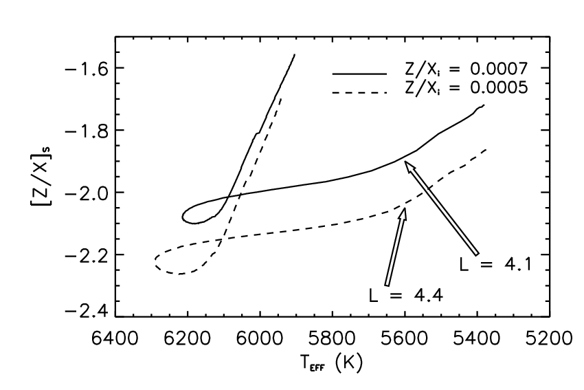


Each stellar evolution model is defined by a set of input model parameters — mass , initial helium content , initial metal to hydrogen ratio , age , the mixing-length parameter , and the extra-mixing coefficient — and these result in model observables, such as a model and a model . By varying the input parameters we aimed to find models that fitted the derived , , and [M/H] as given in Tables 6 and 11.
7.2 Approximate parameters of HD 140283 using

The luminosity provides a very important constraint on the evolution stage of the star. Because it is a measure of the energy production in the star, we can ignore the mixing-length parameter which is relevant only to the outer convective envelope and hence and . In Fig. 6 we show the evolution of luminosity as a function of age, for models of different mass (denoted with a number) and changing and , with the reference model of 0.80 M⊙ having = 0.245 and = 0.0005. We also highlight the error bars associated with when we adopt the reddened and unreddened bolometric flux (reddened is a higher value). We have limited the age range to a minimum expected value, i.e. the minimal age of the old galactic clusters 10 Gyr.
Using only the luminosity, Fig. 6 illustrates the following: 1) The mass of the star is between 0.78 and 0.84 M⊙ if we adopt a minimum = 0.245, consistent with a primordial value predicted by Big Bang nucleosynthesis. 2) Increasing by 0.0002 (typical error, see next section) changes the age by about 0.3 Gyr. 3) The effect of increasing to an upper limit of 0.260 (= , where is indicated in Fig. 6) leads to a corresponding decrease in the age of the reference model by 1.5 Gyr if everything else is left fixed, and imposing an approximate age of the Universe would decrease the lower limit in the mass to 0.75 M⊙. Figure 6 depicts the approximate correlations between and , given just the luminosity constraint. In this figure, we have denoted an upper age limit of Gyr (approximately the age of the Universe) by the dotted horizontal bars for each which imposes a lower limit in mass. We then depict the upper limit in mass when we assume that Halo stars should have begun forming at approximately Gyr (continuous lines), and when we relax this constraint to the age of the youngest globular clusters of Gyr (dashed lines). Using this assumption along with the assumption that the initial helium abundance is low (), we obtain a model-dependent mass of HD 140283 of between 0.75 and 0.84 M⊙. This then implies = 3.65 0.03 by imposing from this work.
7.3 Refining the parameters using the angular diameter constraint
7.3.1 Constraining the mixing-length parameter
The radius and the of a star are extremely sensitive to the adopted mixing-length parameter which parametrizes convection in the convective envelope. It is an adjustable parameter and it needs to be tuned to fit the observational constraints. However, because of the correlations among different parameters and sets of input physics to models, in many cases it is left as a fixed parameter, and its value is set to the value obtained by calibration of the solar parameters with the same physics. This is also the case for many isochrones that are available publicly. While adopting as the solar-calibrated value may be valid for stars that are similar to the Sun, for metal-poor evolved stars (different , , and [Fe/H]) this is certainly not the case as has been shown by Casagrande et al. (2007), for example, who suggest a downward revision for metal-poor stars, or Kervella et al. (2008) for 61 Cyg, or more recently by Creevey et al. (2012) for two metal-poor stars, and from asteroseismology for a few tens of stars, e.g. Metcalfe et al. (2012); Mathur et al. (2012); Bonaca et al. (2012). Fixing with a solar calibrated value for HD 140283 yields no models consistent with observations. However, as we know that the age of HD 140283 is high ( Gyr) and its mass is relatively well-determined as argued in the above paragraph ( M⊙), along with its metallicity, is one of the free parameters that we can in fact constrain, as well as further constraining its age and mass.
In order to reproduce the and of HD 140283, it was necessary to
decrease the value of to about 1.00 (solar value 2.0).
Figure 7 illustrates how the value of is constrained
by the stellar evolution models.
We show the HR diagram depicting the position of the error box of
the reddened solution.
Assuming = 0.245 the mass is between 0.78 and 0.84 M⊙ (see Fig. 6, right panel).
We plot as continuous lines a 0.78 (blue), 0.80 (black), and 0.82 (green)
M⊙ model with a mixing-length
parameter of .
Increasing to 1.30 results in the 0.78 M⊙ evolution track falling inside the
observed constraints (blue dashed).
Decreasing to 0.70 for the 0.82 M⊙ also results in the track falling
within the error box (green dashed).
Directly from the models we can establish a plausible range of for
a given mass for = 0.245:
– 0.78 M⊙ implies ,
– 0.80 M⊙ implies , and
– 0.82 M⊙ implies .
The black dashed line above the error box shows a 0.84 M⊙ model with
a value of .
We were unable to make exolutionary tracks with values of , thus
establishing a model-dependent lower limit on its value, and restricting
the mass of the model to M⊙.
We can summarize as a function of by using the following relation ( 0.01) M⊙ or alternatively as ( 0.2) where the errors are the 1 uncorrelated errors. With a mass between 0.78 and 0.83 M⊙ and between 0.5 and 1.50, we set our reference model to the mean mass M⊙ which implies . This is the solution adopted for = 0.245 (Table 12), and for comparison with other solutions we adopt as the reference value.
7.3.2 Mass, initial helium, and age of the non-reddened star
Figure 8, left panel shows the HR diagram error box and stellar models that satisfy or are close to the unreddened solution. The most central model corresponds to a mass of M⊙, an initial helium abundance of , initial metallicity , and . We also highlight models of other masses (blue) with the same , , and that pass through or close to the error box. Models considering different and (green dashed lines) are also shown. We apply the approach from the previous section to establish a relationship between and , and we also take into account. Given two of the third can be derived as
| (5) |
| (6) |
| (7) |
where these equations must satisfy , and . Using the reference we give two solutions in Table 12 corresponding to = 0.245 (model 1, M1), and = 0.255 (model 2, M2), resulting in masses of 0.78 and 0.77 M⊙.
To determine the age and other properties corresponding to these models we consider the properties of all of the models that pass through the 1 error box. These properties are given in the lower part of Table 12 along with their uncertainties. For M1 we obtain an age of 13.68 Gyr with [M/H] = –2.03.


7.3.3 Mass, initial helium and age of the reddened star
Figure 8 right panel illustrates the optimal models that satisfy the , and [M/H] constraints (central continuous error box) for the reddened solution. The dotted error box shows the position of the unreddened constraints. Following the approach above we establish equations for deriving one of as a function of the other two.
| (8) |
| (9) |
| (10) |
where the equations must satisfy , and . In Sect. 7.3.1 we found an optimal model of M⊙ for = 0.245, and adopting the reference , we obtain M⊙ for = 0.255. The ages of these models are 12.17 and 11.95 Gyr respectively with metallities of [M/H] = –2.06 and –2.07. These properties are summarized in the lower part of Table 12 under the column headings M3 and M4.
| Parameter | Value | Uncertainty | |
|---|---|---|---|
| 0.245 | 0.255 | ||
| AV = 0.00 mag | M1 | M2 | |
| (M⊙) | 0.780 | 0.770 | 0.010 |
| 0.0005 | 0.0005 | 0.0002 | |
| 1.00 | 1.00 | 0.20 | |
| (Gyr) | 13.68 | 13.45 | 0.71 |
| (cm s-2) | 3.64 | 3.64 | 0.03 |
| (L⊙) | 4.12 | 4.12 | 0.10 |
| (K) | 5571 | 5601 | 101 |
| (R⊙) | 2.18 | 2.16 | 0.08 |
| (dex) | –2.03 | –2.05 | 0.07 |
| AV = 0.10 mag | M3 | M4 | |
| (M⊙) | 0.805 | 0.795 | 0.010 |
| 0.0005 | 0.0005 | 0.0002 | |
| 1.00 | 1.00 | 0.20 | |
| (Gyr) | 12.17 | 11.95 | 0.62 |
| (cm s-2) | 3.65 | 3.65 | 0.02 |
| (L⊙) | 4.42 | 4.42 | 0.10 |
| (K) | 5662 | 5695 | 105 |
| (R⊙) | 2.20 | 2.18 | 0.08 |
| (dex) | –2.06 | –2.07 | 0.05 |
7.3.4 The global solution
The determination of precise stellar properties that cannot be observed is extremely difficult, particularly because of the strong correlations between , and , and consequently the age. The luminosity constraint along with the stellar models and the assumptions on the allowed age range of the star refined the mass to and consequently to 3.65 0.03. The angular diameter then further constrained to within a range of 0.5 – 1.5 and to , but most importantly it provided a tight correlation between them, along with . Our models have a surface metallicity of [M/H] , in good agreement with the observed one (–2.10).
Determining the age of the star depends on the adopted values of of , where only two are independent and the third is calculated from Eqs. 5–10. The full range of mass values (by varying and ) has the largest impact on the determination of age, followed by . The value of only indirectly influences the age through the required change of and . To attempt to quantify this effect, in Figure 9 we show the ages of the models that fit the observational constraints for a range of parameters. We varied the mass (x-axis) and (circles: = 0.245, diamonds: = 0.255) within the allowed correlations as shown in Fig. 6. For each combination we adjusted to within its allowed range until the evolution track passed through the centre of the error box. This was done for the reddened solution (shown in red) and the unreddened solution (black). The figure shows the age of the models for these combinations. The crosses show the solutions in Table 12 (the central models in Fig. 8).
Allowing for all plausible combinations of results in a possible age of HD 140283 varying between 10.5 Gyr and 14.0 Gyr, with a lower limit of just under 11 Gyr for the zero reddened solution. The required values of are systematically lower for the zero reddened solution with a typical value of while the reddened solution requires .
We can parametrize the age as a function of , and AV using the following equation
| (11) |
where , , , and the combination of and necessarily implies . The value of can be approximated by
| (12) |
and is restricted to values between 0.5 and 1.5 (lower values for higher masses and vice versa). The full range of ages and for all combinations of are given in the on-line version.
Here it is clear that in order to determine the age of the star with the best precision we need to restrict the values of one of the parameters (see Sect. 8). Resolving the reddening problem would also relieve this degeneracy.

Assuming that the mixing-length parameter does not vary much within the atmospheric parameters of our models ( = 3.65, [M/H] , – 5660 K), and by requiring that the different solutions adopt a similar value, we can judge the impact of reddening and on the mass and age determination. Table 12 shows four solutions that adopt for two values of and the two extreme values of AV. The effect of increasing by 0.01 is a decrease in the mass and the age by 0.01 M⊙ and Gyr. The biggest difference comes from the adopted reddening, giving a 1.5 Gyr difference between the solutions with AV = 0.0 and 0.1 mag. In principle we may expect to be able to impose a value of in the near future either from the calibration of this parameter with large samples of targets, e.g. from asteroseismology (Bonaca et al. 2012; Metcalfe et al. 2014), or from advances in 3D numerical techniques, e.g. Trampedach & Stein (2011). Imposing this parameter externally would reduce the total range of mass, , and possibly extinction, thus delivering a more reliable determination of its age.
The uncertainties that we give in Table 12 for , , and are the 1 uncorrelated uncertainties. These are obtained by fixing the parameters and varying the one of interest until we reach the edge of the error box. The uncertainties in the other parameters are obtained by varying the above-mentioned parameters up to 1 at the same time and requiring that they remain within the error box, e.g. for solution M3 the mass took values of between (0.815 - 0.790)/2 M⊙ (rounded), while varied between 1.2 and 0.8, and between 0.0003 and 0.0007.
8 Discussion
8.1 Observational results
In this work we determined three important quantities for HD 140283: the angular diameter , the bolometric flux , and a 1D LTE derived from H line wings. Combining the first two observational results with a well-measured parallax from Bond et al. (2013) yields the stellar parameters , , , and . In this work we found that the biggest contributor to our systematic error in and is the existence or not of interstellar reddening. The adoption of zero or non-zero reddening leads to a change in and by 0.3 L⊙ and 100 K, respectively. The determination of the spectroscopic led to a value closer to the reddened solution (5626 K). If we used this spectroscopic value to deduce and thus reddening (using the angular diameter), we would obtain = 4.16 x 10⁻⁸ erg s-1 cm-2, giving a flux excess of 0.27 x10⁻⁸ and corresponding to AV 0.084 mag or E(B-V) = 0.027 mag by adopting an extinction law of R(V) = 3.1. This value would be in agreement with the value proposed by Bond et al. (2013).
8.2 1D LTE spectroscopic
In this work we determined a 1D LTE spectroscopic using H line wings while imposing = 3.65 0.06 and [Fe/H] = –2.46 0.14. The was imposed from this work using the interferometric and an estimate of M⊙, later confirmed with models to be correct. The question we posed was whether such an analysis is capable of determining of metal-poor stars where generally missing physics in atmospheric models can lead to a large variety of determinations with correlations between the parameters. In Figure 10 we show determinations of the spectroscopic parameters from various authors as provided by the PASTEL catalogue (Soubiran et al. 2010). We show the [Fe/H] determinations against with a colour and symbol code corresponding to different . The blue filled circles are those with corresponding to the constraints we can impose from this work (in many cases their was constrained prior to the analysis). The black circle marks our determination of . The shaded background illustrates the determination of the interferometric assuming reddening, and the dashed lines illustrate the boundaries with an assumption of zero reddening. If we can show that we need to consider reddening then we can conclude that the spectroscopic analysis is indeed capable of reproducing the of such metal-poor stars, if we can impose a reliable constraint such as .
Recently Ruchti et al. (2013) studied systematic biases in determinations, and they found that the determined from H were hotter than those derived from the angular diameter for metal-poor stars by 40 – 50 K (including HD 140283). Our results are in agreement with this statement if we assume some mild absorption to the star, e.g. mag.
For HD 140283, Ruchti et al. (2013) used surface brightness relations to estimate the interferometric for this star (5720 K), and they obtained an H = 5775 K, 150 K hotter than ours. There are a few explanations for this difference: 1) the and [Fe/H] values adopted affect the derived (see Table 10); however, they did not specify these values in their work; 2) the observations give different results — our analysis with NARVAL data yields higher than the other three sets; 3) the theoretical profiles were calculated using different model atmospheres and code; and 4) self-broadening was computed using a different (older) theory. We believe that our analysis using different line masks and four sets of observations should yield a more reliable result. The only way to unveil the origin of the systematic difference is to use each other’s observations and compare the results.

8.3 Initial metallicity and the extra-mixing parameter in stellar models
The mean surface metallicity of our most reliable models is = –2.05, with an initial value of = –1.70 or = 0.0005 (the surface metallicity is mostly set by the initial value with some slight variation due to ). This value was obtained by adopting a diffusion parameter in the stellar models, one that we determined by comparing the difference in surface metallicity abundance of stars at their turn-off stage and the base of the giant branch with observed results from Nordlander et al. (2012) of the globular cluster NGC 6397. However, as it still remains an adjustable parameter in the stellar models, it could be incorrect. Adopting a much smaller value results in a maximum change in surface metallicity during main sequence evolution of up to 1.0 dex (see e.g. Fig. 5 which shows a maximum change of 0.55 dex). This would require an initial value of the order of –1.40 dex. This scenario is improbable and would result in a surface metallicity difference between turn-off and giant stars in disagreement with Nordlander et al. (2012). Adopting a larger value for the parameter would reduce the maximum change in surface metallicity during evolution, and converging on a surface value of –2.10 dex would require the initial value to be decreased, for example to –1.90 dex or = 0.0002. For a star with an age almost the age of the Galaxy (adopting zero reddening) a lower initial metallicity could be more likely. However, a star 1 billion years younger could be consistent with a higher initial metallicity. The impact of this change of physics and metallicity on the resulting stellar properties is currently limited by our observational errors. At the moment we cannot explore this further and we are required to impose the external constraints.
8.4 Improving the precision and accuracy of the age
It is clear that in order to determine the most accurate and precise age for HD 140283, it is necessary to solve the extinction problem, and to reduce the span of masses that pass through the error box. The second question can be addressed by obtaining a more precise determination of the angular diameter. From Fig. 8 one can immediately see that by reducing the error bar in by a factor of two, fewer models would satisfy the constraints. As an example, the right panel shows that models of masses between 0.790 and 0.805 (a total span of 0.015 M⊙) would be the only models that pass through the error box of half of its size. The parallax and already contribute very little to the error bar for and , and so the only option is to obtain a precision in of the order of 0.007 mas. By cutting both the external and the statistical errors in half, this precision could be achieved. The current precision is just under 4%, which is excellent considering that we are already working at the limits of angular resolution using the CHARA array with VEGA and VEGA’s sensitivity limits. However, the telescopes of the CHARA array will be equipped with adaptative optic (AO) systems in the next one or two years. This will improve both the sensitivity and measurement precision of VEGA. The gain in sensitivity would allow us to observe fainter (so smaller) calibrators, hence reduce the external error affecting the calibrated visibilities. New observations of HD140283 with CHARA/VEGA or CHARA/FRIEND (future instrument) equipped with AO would allow us to achieve the necessary precision.

8.5 Improving the mass and age from asteroseismology
Another way to determine the mass of the star is through the detection and interpretation of stellar oscillation frequencies. Acoustic oscillation frequencies (sound waves) are sensitive to the sound speed profile of the star and thus its density structure and mean density. Because has been measured, in-depth asteroseismic analysis would allow a very high precision model-dependent determination of the mass. In Fig. 11 we show the relative differences between the sound speed profiles (from 0.02 to 0.8 the stellar radius) for the M3 and M1 models, (M3-M1)/M3. This represents the difference between the reddened and unreddened solution for (continuous). At the same time, we also show the difference between the reddened solutions with different initial helium abundance, M3 and M4 (dashed). The largest differences for both cases are found very close to the centre of the star and near the outer convection zone. These differences cause changes in the frequencies of the oscillation modes that can be detected, e.g. a radial high-order mode () has a predicted frequency of 1240.2 Hz for M3 and this same mode for M1 is 1251.0 Hz, although for the M4 model (different ) it is 1240.7 Hz, not distinguishable from the M3 solution at current asteroseismic modelling limitations (e.g. Kjeldsen et al. 2008b). Precision in asteroseismic frequencies are well below 1.0 Hz, even for a ten-day ground-based observational campaign. Stellar oscillations have been detected in stars of this mass. At this stage of evolution, the so-called g-modes are very sensitive to the core conditions and hence should be able to distinguish even more clearly between both models. However, we need to verify whether there are sufficient metallic lines in the spectrum to accurately detect radial velocity shifts (the oscillations).
8.5.1 Detection of oscillations in metal-poor stars
The star Ind has a similar mass to HD 140283, but has a higher metallicity ([M/H] = –1.3). This star was the subject of a radial velocity asteroseismic campaign using telescopes in Australia and Chile and solar-like oscillations were detected (Bedding et al. 2006; Carrier et al. 2007). The oscillations were analysed and the amplitudes of the frequencies were in the range 50-170 cm s-1 (the solar amplitudes are of the order of 23 cm s-1, see also Kjeldsen et al. (2008a) for a more recent analysis of the amplitudes of both of these stars). A recent asteroseismic observational campaign of a different star using the SOPHIE spectrograph at the Observatoire Haute Provence in February 2013 allowed us to reach a precision of 20-25 cm s-1 in the power spectrum for a total of 8 good nights out of 12 assigned. The detections of such oscillation frequencies are clearly very feasible using different instruments or telescopes. Oscillations are detectable in metal-poor stars, but how metal-poor is observationally possible? HD 140283 would be an ideal target for continued observations, because the non-detection of oscillations would impose an upper limit on the amplitudes of the modes in metal-poor stars, while the detection of oscillation frequencies would provide valuable constraints on the mass and age of this star, and stellar interior models.
9 Conclusions
In this work we determined stellar properties of HD 140283 by measuring the angular diameter of the star and performing bolometric flux fitting. The measured diameter is mas and coupling this with a parallax of mas from Bond et al. (2013) we obtain a linear radius of the star R⊙ and = 3.65 0.06. The bolometric flux fitting resulted in two solutions, one where interstellar extinction AV = 0.0 mag, and the other with a maximum non-zero value of 0.1 mag. Adopting these two values we derived (4.12 or 4.47 L⊙), (5534 or 5647 K), bolometric corrections, and the absolute magnitude (Table 6). We also determined a spectroscopic using a 1D LTE analysis fitting H line wings and we found a value of 5626 K, a value more compatible with the interferometric assuming a small amount of reddening. If is indeed a higher value because of interstellar reddening, this is a very important result as it shows that a 1D LTE analysis of H wings yields accurate at this low-metallicity regime. Our measured angular diameter is larger by about 2 than that predicted by the surface brightness relations of Kervella et al. (2004), suggesting that indeed more determinations of are needed for such metal-poor and/or evolved objects to more accurately calibrate this scale, especially important with the advent of Gaia and with the availability of precise distance measurements for a billion stars in the next five years.
By interpreting the observational results using stellar models we derived a strict relationship between mass , mixing-length parameter , and initial helium abundance (Eqs. 5–10), where only two are independent. We further determined the age of the star for all possible combinations of these parameters; Eq. 11 parametrizes as a function of the adopted , (implying ), and reddening AV. Fixing we studied the impact of changing and AV on the final solution. For AV = 0.10 mag we obtain = 0.805 0.010 M⊙, corresponding to an age of 12.17 0.69 Gyr. For AV = 0.00 mag we obtain a slightly lower mass of = 0.780 0.010 M⊙, corresponding to an age of 13.68 0.61 Gyr (fixing = 0.245). The impact of is much smaller, causing a decrease in and of 0.01 M⊙ and 0.2 Gyr. Table 12 summarizes some of our modelling results, while the on-line version gives the full range of parameter solutions.
By adopting zero or very little reddening Bond et al. (2013) and VandenBerg et al. (2014) derive an age of 14.3 Gyr in a completely independent manner. These results were obtained by adopting an oxygen abundance which was derived with a higher than the one determined in this work. In their work, the mixing-length parameter was not explored in their models and this would shift the evolution tracks towards lower , thus providing a match to the observational data at a lower age. Casagrande et al. (2011) in an independent manner derive an age of 13.8 Gyr and 13.9 Gyr assuming no reddening and using the BaSTI (Cordier et al. 2007) and PADOVA (Bertelli et al. 2008) isochrones. These determinations of the age of HD 140283 give an indication of the systematic error we can expect on stellar ages by using different approaches and assumptions on both the data and models.
For all of our stellar models we needed to adapt the mixing-length parameter to a value much lower than the Sun, i.e. from 2.0 to 1.0 using the Eggleton (1972) treatment of mixing-length. If reddening is non-existent, then takes a lower value () on average. This result reinforces previously published results of the non-universality of the mixing-length parameter, e.g. Miglio & Montalbán (2005), one that is generally fixed in published stellar evolution tracks/isochrones. We note that our somewhat lower (compared to some recent determinations of 5700 K and higher) along with the observed Li abundances provides an important reference point for studying Li versus for metal-poor stars (see e.g. Charbonnel & Primas (2005) , their Fig. 12) and consequently Li surface depletion scenarios.
The next crucial steps to better understand this star and to decorrelate the stellar properties of mass, age, initial helium abundance, and to look at the treatment of diffusion in such stars, is to reduce the uncertainty on the angular diameter by at least a factor of two, and to perform asteroseismic observations to better recover the internal profile of the star and hence its mass and age. Predictions of the mixing-length parameter from external constraints would also lead to a large improvement in determining mass, initial helium, and age. All of these are realistic with current numerical capabilities and current or near-future instrumentation. One of the biggest improvements to the age and mass determinations, however, relies on the exact knowledge of extinction between the Earth and this star.
Acknowledgements.
This paper is dedicated to the wonderful astronomer Olivier Chesneau. We thank Isabelle Tallon-Bosc for detailed discussions regarding uncertainties in interferometric data. We thank the VEGA observing group at the Observatoire de la Côte d’Azur (OCA) in Nice, France (remote observing) and at CHARA, California, USA. The work by the SAM (http://www.astro.uu.se/~ulrike/GaiaSAM/) group in defining a set of benchmark stars is greatly appreciated. The CHARA Array is funded by the National Science Foundation through NSF grant AST-0908253 and by Georgia State University through the College of Arts and Sciences. TSB acknowledges support provided through NASA grant ADAP12-0172. UH acknowledges support from the Swedish National Space Board (Rymdstyrelsen). PK acknowledges the support of PHASE, the high angular resolution partnership between ONERA, Observatoire de Paris, CNRS and the Université Denis Diderot, Paris 7. We acknowledge financial support from the “Programme National de Physique Stellaire" (PNPS) of CNRS/INSU, France. During part of this research OLC was a Henri Poincaré Fellow at OCA, which is funded by the Conseil Général des Alpes-Maritimes and OCA.References
- Alexander & Ferguson (1994) Alexander, D. R. & Ferguson, J. W. 1994, ApJ, 437, 879
- Ali & Griem (1966) Ali, A. W. & Griem, H. R. 1966, Physical Review, 144, 366
- Allard et al. (2008) Allard, N. F., Kielkopf, J. F., Cayrel, R., & van’t Veer-Menneret, C. 2008, A&A, 480, 581
- Alonso et al. (1996) Alonso, A., Arribas, S., & Martinez-Roger, C. 1996, A&AS, 117, 227
- Angulo (1999) Angulo, C. 1999, in American Institute of Physics Conference Series, Vol. 495, American Institute of Physics Conference Series, 365–366
- Arenou et al. (1992) Arenou, F., Grenon, M., & Gomez, A. 1992, A&A, 258, 104
- Aurière (2003) Aurière, M. 2003, in EAS Publications Series, Vol. 9, EAS Publications Series, ed. J. Arnaud & N. Meunier, 105
- Bagnulo et al. (2003) Bagnulo, S., Jehin, E., Ledoux, C., et al. 2003, The Messenger, 114, 10
- Bailer-Jones et al. (2013) Bailer-Jones, C. A. L., Andrae, R., Arcay, B., et al. 2013, A&A, 559, A74
- Baker (2008) Baker, J. 2008, Natl. Inst. Stand. Technol. Technical Note, 1612
- Ballester et al. (2000) Ballester, P., Modigliani, A., Boitquin, O., et al. 2000, The Messenger, 101, 31
- Barklem et al. (2000) Barklem, P. S., Piskunov, N., & O’Mara, B. J. 2000, A&A, 355, L5
- Bedding et al. (2006) Bedding, T. R., Butler, R. P., Carrier, F., et al. 2006, ApJ, 647, 558
- Bennett et al. (2013) Bennett, C. L., Larson, D., Weiland, J. L., et al. 2013, ApJS, 208, 20
- Bertelli et al. (2008) Bertelli, G., Girardi, L., Marigo, P., & Nasi, E. 2008, A&A, 484, 815
- Bigot et al. (2006) Bigot, L., Kervella, P., Thévenin, F., & Ségransan, D. 2006, A&A, 446, 635
- Bigot et al. (2011) Bigot, L., Mourard, D., Berio, P., et al. 2011, A&A, 534, L3
- Blanco-Cuaresma et al. (2014) Blanco-Cuaresma, S., Soubiran, C., Jofré, P., & Heiter, U. 2014, A&A, 566, A98
- Bonaca et al. (2012) Bonaca, A., Tanner, J. D., Basu, S., et al. 2012, ApJ, 755, L12
- Bond et al. (2013) Bond, H. E., Nelan, E. P., VandenBerg, D. A., Schaefer, G., & Harmer, D. 2013, in American Astronomical Society Meeting Abstracts, Vol. 221, American Astronomical Society Meeting Abstracts, 443.08
- Bonifacio & Molaro (1998) Bonifacio, P. & Molaro, P. 1998, ApJ, 500, L175
- Bonneau et al. (2006) Bonneau, D., Clausse, J.-M., Delfosse, X., et al. 2006, A&A, 456, 789
- Boyajian et al. (2014) Boyajian, T. S., van Belle, G., & von Braun, K. 2014, AJ, 147, 47
- Brown & Gilliland (1994) Brown, T. M. & Gilliland, R. L. 1994, ARA&A, 32, 37
- Burgers (1969) Burgers, J. M. 1969, Flow Equations for Composite Gases, ed. Burgers, J. M.
- Cardelli et al. (1989) Cardelli, J. A., Clayton, G. C., & Mathis, J. S. 1989, ApJ, 345, 245
- Carney & Latham (1987) Carney, B. W. & Latham, D. W. 1987, AJ, 93, 116
- Carrier et al. (2007) Carrier, F., Kjeldsen, H., Bedding, T. R., et al. 2007, A&A, 470, 1059
- Casagrande et al. (2007) Casagrande, L., Flynn, C., Portinari, L., Girardi, L., & Jimenez, R. 2007, MNRAS, 382, 1516
- Casagrande et al. (2014) Casagrande, L., Portinari, L., Glass, I. S., et al. 2014, MNRAS
- Casagrande et al. (2010) Casagrande, L., Ramírez, I., Meléndez, J., Bessell, M., & Asplund, M. 2010, A&A, 512, A54
- Casagrande et al. (2011) Casagrande, L., Schönrich, R., Asplund, M., et al. 2011, A&A, 530, A138
- Cayrel et al. (2011) Cayrel, R., van’t Veer-Menneret, C., Allard, N. F., & Stehlé, C. 2011, A&A, 531, A83
- Charbonnel & Primas (2005) Charbonnel, C. & Primas, F. 2005, A&A, 442, 961
- Chiavassa et al. (2012) Chiavassa, A., Bigot, L., Kervella, P., et al. 2012, A&A, 540, A5
- Chiavassa et al. (2009) Chiavassa, A., Plez, B., Josselin, E., & Freytag, B. 2009, A&A, 506, 1351
- Claret et al. (2012) Claret, A., Hauschildt, P. H., & Witte, S. 2012, A&A, 546, A14
- Collet et al. (2009) Collet, R., Nordlund, Å., Asplund, M., Hayek, W., & Trampedach, R. 2009, Mem. Soc. Astron. Italiana, 80, 719
- Cordier et al. (2007) Cordier, D., Pietrinferni, A., Cassisi, S., & Salaris, M. 2007, AJ, 133, 468
- Cousins (1984) Cousins, A. W. J. 1984, South African Astronomical Observatory Circular, 8, 59
- Creevey et al. (2013) Creevey, O. L., Thévenin, F., Basu, S., et al. 2013, MNRAS, 431, 2419
- Creevey et al. (2012) Creevey, O. L., Thévenin, F., Boyajian, T. S., et al. 2012, A&A, 545, A17
- Dekker et al. (2000) Dekker, H., D’Odorico, S., Kaufer, A., Delabre, B., & Kotzlowski, H. 2000, in Society of Photo-Optical Instrumentation Engineers (SPIE) Conference Series, Vol. 4008, Society of Photo-Optical Instrumentation Engineers (SPIE) Conference Series, ed. M. Iye & A. F. Moorwood, 534–545
- Donati et al. (1997) Donati, J., Semel, M., Carter, B. D., Rees, D. E., & Collier Cameron, A. 1997, MNRAS, 291, 658
- Drozdowski et al. (1997) Drozdowski, R., Ignaciuk, M., Kwela, J., & Heldt, J. 1997, Zeitschrift fur Physik D Atoms Molecules Clusters, 41, 125
- Eggleton (1972) Eggleton, P. P. 1972, MNRAS, 156, 361
- Eggleton et al. (1973) Eggleton, P. P., Faulkner, J., & Flannery, B. P. 1973, A&A, 23, 325
- Epstein et al. (2014) Epstein, C. R., Elsworth, Y. P., Johnson, J. A., et al. 2014, ApJ, 785, L28
- Flower (1996) Flower, P. J. 1996, ApJ, 469, 355
- Fuhrmann (1998) Fuhrmann, K. 1998, A&A, 330, 626
- Fukugita et al. (1995) Fukugita, M., Shimasaku, K., & Ichikawa, T. 1995, PASP, 107, 945
- Gallagher et al. (2010) Gallagher, A. J., Ryan, S. G., García Pérez, A. E., & Aoki, W. 2010, A&A, 523, A24
- Gilmore et al. (2012) Gilmore, G., Randich, S., Asplund, M., et al. 2012, The Messenger, 147, 25
- González Hernández & Bonifacio (2009) González Hernández, J. I. & Bonifacio, P. 2009, A&A, 497, 497
- Gray (2005) Gray, D. F. 2005, The Observation and Analysis of Stellar Photospheres
- Grevesse & Noels (1993) Grevesse, N. & Noels, A. 1993, in Origin and Evolution of the Elements, ed. N. Prantzos, E. Vangioni-Flam, & M. Casse, 15–25
- Griersmith (1980) Griersmith, D. 1980, AJ, 85, 789
- Grundahl et al. (2000) Grundahl, F., VandenBerg, D. A., Bell, R. A., Andersen, M. I., & Stetson, P. B. 2000, AJ, 120, 1884
- Gustafsson et al. (2008) Gustafsson, B., Edvardsson, B., Eriksson, K., et al. 2008, A&A, 486, 951
- Gustafsson et al. (2003) Gustafsson, B., Edvardsson, B., Eriksson, K., et al. 2003, in Astronomical Society of the Pacific Conference Series, Vol. 288, Stellar Atmosphere Modeling, ed. I. Hubeny, D. Mihalas, & K. Werner, 331
- Hauck & Mermilliod (1990) Hauck, B. & Mermilliod, M. 1990, A&AS, 86, 107
- Hauck et al. (1995) Hauck, B., Nitschelm, C., Mermilliod, M., & Mermilliod, J. C. 1995, VizieR Online Data Catalog, 2167, 0
- Hauschildt et al. (1999) Hauschildt, P. H., Allard, F., Ferguson, J., Baron, E., & Alexander, D. R. 1999, ApJ, 525, 871
- Haywood et al. (2013) Haywood, M., Di Matteo, P., Lehnert, M. D., Katz, D., & Gómez, A. 2013, A&A, 560, A109
- Houdashelt et al. (2000) Houdashelt, M. L., Bell, R. A., & Sweigart, A. V. 2000, AJ, 119, 1448
- Huber et al. (2012) Huber, D., Ireland, M. J., Bedding, T. R., et al. 2012, ApJ, 760, 32
- Husser et al. (2013) Husser, T.-O., Wende-von Berg, S., Dreizler, S., et al. 2013, A&A, 553, A6
- Jofré et al. (2014) Jofré, P., Heiter, U., Soubiran, C., et al. 2014, A&A, 564, A133
- Kervella et al. (2008) Kervella, P., Mérand, A., Pichon, B., et al. 2008, A&A, 488, 667
- Kervella et al. (2004) Kervella, P., Thévenin, F., Di Folco, E., & Ségransan, D. 2004, A&A, 426, 297
- Kjeldsen & Bedding (1995) Kjeldsen, H. & Bedding, T. R. 1995, A&A, 293, 87
- Kjeldsen et al. (2008a) Kjeldsen, H., Bedding, T. R., Arentoft, T., et al. 2008a, ApJ, 682, 1370
- Kjeldsen et al. (2008b) Kjeldsen, H., Bedding, T. R., & Christensen-Dalsgaard, J. 2008b, ApJ, 683, L175
- Korn et al. (2007) Korn, A. J., Grundahl, F., Richard, O., et al. 2007, ApJ, 671, 402
- Kurucz (2010) Kurucz, R. L. 2010, Robert L. Kurucz on-line database of observed and predicted atomic transitions, http://kurucz.harvard.edu/atoms/2200/gfemq2200.pos, http://kurucz.harvard.edu/atoms/2201/gfemq2201.pos
- Lallement et al. (2014) Lallement, R., Vergely, J.-L., Valette, B., et al. 2014, A&A, 561, A91
- Lebreton (2000) Lebreton, Y. 2000, ARA&A, 38, 35
- Lebreton & Goupil (2014) Lebreton, Y. & Goupil, M. J. 2014, A&A, 569, A21
- Lejeune et al. (1997) Lejeune, T., Cuisinier, F., & Buser, R. 1997, VizieR Online Data Catalog, 412, 50229
- Masana et al. (2006) Masana, E., Jordi, C., & Ribas, I. 2006, A&A, 450, 735
- Mathur et al. (2012) Mathur, S., Metcalfe, T. S., Woitaszek, M., et al. 2012, ApJ, 749, 152
- May et al. (1974) May, M., Richter, J., & Wichelmann, J. 1974, A&AS, 18, 405
- Mayor et al. (2003) Mayor, M., Pepe, F., Queloz, D., et al. 2003, The Messenger, 114, 20
- McMillan et al. (1976) McMillan, R. S., Breger, M., Ferland, G. J., & Loumos, G. L. 1976, PASP, 88, 495
- Meléndez et al. (2010) Meléndez, J., Ramírez, I., Casagrande, L., et al. 2010, Ap&SS, 328, 193
- Mermilliod (1986) Mermilliod, J.-C. 1986, Catalogue of Eggen’s UBV data., 0 (1986), 0
- Metcalfe et al. (2012) Metcalfe, T. S., Chaplin, W. J., Appourchaux, T., et al. 2012, ApJ, 748, L10
- Metcalfe et al. (2009) Metcalfe, T. S., Creevey, O. L., & Christensen-Dalsgaard, J. 2009, ApJ, 699, 373
- Metcalfe et al. (2014) Metcalfe, T. S., Creevey, O. L., Doğan, G., et al. 2014, ApJS, 214, 27
- Miglio & Montalbán (2005) Miglio, A. & Montalbán, J. 2005, A&A, 441, 615
- Morel & Magnenat (1978) Morel, M. & Magnenat, P. 1978, A&AS, 34, 477
- Morel (1997) Morel, P. 1997, A&AS, 124, 597
- Morel & Lebreton (2008) Morel, P. & Lebreton, Y. 2008, Ap&SS, 316, 61
- Morel & Thévenin (2002) Morel, P. & Thévenin, F. 2002, A&A, 390, 611
- Mourard et al. (2011) Mourard, D., Bério, P., Perraut, K., et al. 2011, A&A, 531, A110
- Mourard et al. (2012) Mourard, D., Challouf, M., Ligi, R., et al. 2012, in Society of Photo-Optical Instrumentation Engineers (SPIE) Conference Series, Vol. 8445, Society of Photo-Optical Instrumentation Engineers (SPIE) Conference Series
- Nordlander et al. (2012) Nordlander, T., Korn, A. J., Richard, O., & Lind, K. 2012, ApJ, 753, 48
- Norris et al. (1985) Norris, J., Bessell, M. S., & Pickles, A. J. 1985, ApJS, 58, 463
- O’Donnell (1994) O’Donnell, J. E. 1994, ApJ, 422, 158
- Perryman (2005) Perryman, M. A. C. 2005, in Astronomical Society of the Pacific Conference Series, Vol. 338, Astrometry in the Age of the Next Generation of Large Telescopes, ed. P. K. Seidelmann & A. K. B. Monet, 3
- Pickles (1998a) Pickles, A. J. 1998a, VizieR Online Data Catalog, 611, 863
- Pickles (1998b) Pickles, A. J. 1998b, PASP, 110, 863
- Press et al. (1992) Press, W. H., Teukolsky, S. A., Vetterling, W. T., & Flannery, B. P. 1992, Numerical recipes in FORTRAN. The art of scientific computing
- Ramírez et al. (2010) Ramírez, I., Collet, R., Lambert, D. L., Allende Prieto, C., & Asplund, M. 2010, ApJ, 725, L223
- Rogers & Iglesias (1992) Rogers, F. J. & Iglesias, C. A. 1992, ApJS, 79, 507
- Ruchti et al. (2013) Ruchti, G. R., Bergemann, M., Serenelli, A., Casagrande, L., & Lind, K. 2013, MNRAS, 429, 126
- Ryan (1989) Ryan, S. G. 1989, AJ, 98, 1693
- Salaris et al. (1993) Salaris, M., Chieffi, A., & Straniero, O. 1993, ApJ, 414, 580
- Schuster & Nissen (1989) Schuster, W. J. & Nissen, P. E. 1989, A&A, 221, 65
- Silva Aguirre et al. (2013) Silva Aguirre, V., Basu, S., Brandão, I. M., et al. 2013, ApJ, 769, 141
- Siqueira Mello et al. (2012) Siqueira Mello, C., Barbuy, B., Spite, M., & Spite, F. 2012, A&A, 548, A42
- Skrutskie et al. (2006) Skrutskie, M. F., Cutri, R. M., Stiening, R., et al. 2006, AJ, 131, 1163
- Soubiran et al. (2010) Soubiran, C., Le Campion, J.-F., Cayrel de Strobel, G., & Caillo, A. 2010, A&A, 515, A111
- Sturmann et al. (2010) Sturmann, J., ten Brummelaar, T., Sturmann, L., & McAlister, H. A. 2010, in Society of Photo-Optical Instrumentation Engineers (SPIE) Conference Series, Vol. 7734, Society of Photo-Optical Instrumentation Engineers (SPIE) Conference Series
- ten Brummelaar et al. (2005) ten Brummelaar, T. A., McAlister, H. A., Ridgway, S. T., et al. 2005, ApJ, 628, 453
- Thévenin (1998) Thévenin, F. 1998, VizieR Online Data Catalog, 3193, 0
- Torres (2010) Torres, G. 2010, AJ, 140, 1158
- Trampedach & Stein (2011) Trampedach, R. & Stein, R. F. 2011, ApJ, 731, 78
- Upgren et al. (1992) Upgren, A. R., Zhao, H., & Lee, J. T. 1992, AJ, 104, 1203
- Valenti & Fischer (2005) Valenti, J. A. & Fischer, D. A. 2005, ApJS, 159, 141
- Valenti & Piskunov (1996) Valenti, J. A. & Piskunov, N. 1996, A&AS, 118, 595
- van Belle et al. (2008) van Belle, G. T., van Belle, G., Creech-Eakman, M. J., et al. 2008, ApJS, 176, 276
- van Leeuwen (2007) van Leeuwen, F. 2007, A&A, 474, 653
- VandenBerg et al. (2014) VandenBerg, D. A., Bond, H. E., Nelan, E. P., et al. 2014, ApJ, 792, 110
- von Braun et al. (2012) von Braun, K., Boyajian, T. S., Kane, S. R., et al. 2012, ApJ, 753, 171
- Wahlgren (2010) Wahlgren, G. M. 2010, in EAS Publications Series, Vol. 43, EAS Publications Series, ed. R. Monier, B. Smalley, G. Wahlgren, & P. Stee, 91–114
- Wiese & Fuhr (2009) Wiese, W. L. & Fuhr, J. R. 2009, Journal of Physical and Chemical Reference Data, 38, 565
- Yamada et al. (2013) Yamada, S., Suda, T., Komiya, Y., Aoki, W., & Fujimoto, M. Y. 2013, MNRAS, 436, 1362
- Yi et al. (2001) Yi, S., Demarque, P., Kim, Y.-C., et al. 2001, ApJS, 136, 417
Appendix A Bolometric flux fitting approach 2 (method 2B and 2C)
We describe in detail the second bolometric flux-fitting approach that was implemented in this work. The method incorporates a non-linear least-squares minimization algorithm (Levenberg-Marqwardt) to find the best scaled interpolated spectrum that fits a set of observed flux points or photometric magnitudes (in this work we just use the flux data). The fitting method requires on input a set of initial parameters — , [Fe/H], , E(B-V), and a scaling factor — which define the characteristics of the spectra, the reddening to apply, and ratio of the stellar radius to the star’s distance. These parameters are optimized within the algorithm and the bolometric flux is calculated by numerical integration of the scaled optimal spectrum. The method is designed to allow implementation of any spectral library. In this work we use the BASEL (Lejeune et al. 1997) and PHOENIX libraries (Hauschildt et al. 1999; Husser et al. 2013).
Because of the strong degeneracy between the stellar parameters, in practice we fix three of the values , , [Fe/H], AV, while fitting the fourth along with , so only two stellar parameters are fitted at any one time. Changing and [Fe/H] by 0.5 dex, which is much larger than the typical errors on these values, has a negligible influence on the final calculated bolometric flux . Generally these parameters are the ones that are fixed. Changing AV, however, does have an important effect as explained below.
Within the fitting process, each spectrum is linearly interpolated between adjacent parameter points to the desired parameter values as proposed by the minimization algorithm. We have tested for different interpolation schemes and because of the relatively dense grid spacing (e.g. 100 K or 250 K in , 0.5 in , 0.5 in [Fe/H]) the choice and order of interpolation is irrelevant. The scale factor is also proposed at the same time by the minimization algorithm. A value is then calculated between the observed data and the newly proposed scaled spectrum. If the value improves then the minimization algorithm continues in the same direction. When the fails to improve after four iterations the fitting stops, but convergence is usually reached within only three or four iterations. The final results are not sensitive to the initial parameters; for example, initial values differing by 1000 K yielded consistent results.
To account for reddening we apply reddening laws to the spectra using the Interactive Data Language (IDL) routine ccm_unred and the input E(B-V), along with a choice of extinction laws of , which we fix at 3.1 in this work. This routine is based on the Cardelli et al. (1989) coefficients and updated with O’Donnell (1994) in the UV. The values of and AV are highly degenerate parameters if no external constraints are imposed, and so to determine AV a fitting process is begun allowing only and to be fitted, but imposing a range of values of E(B-V). The fit yielding the smallest defines the adopted E(B-V) and thus AV (using ). The same results are obtained by fixing at different values while fitting E(B-V). If the observed data give a best match to a reddened spectrum, the intrinsic (unreddened) flux of the star is thus larger, indicating a more luminous star.