MIMO Broadcasting for Simultaneous Wireless Information and Power Transfer: Weighted MMSE ApproachesThanks: C. Song is with the Dept. of Information and Communications Eng., Korea National University of Transportation, Chungju, Korea (e-mail: c.song@ut.ac.kr). J. Park is with the Dept. of Electronics Eng., Pukyong National University, Busan, Korea (e-mail: jaehyun@pknu.ac.kr). C. Ling is with the Dept. of Electrical and Electronic Eng., Imperial College, London, UK (e-mail: c.ling@imperial.ac.uk). B. Clerckx is with the Dept. of Electrical and Electronic Eng., Imperial College, London, UK and the School of Electrical Eng., Korea University, Seoul, Korea (e-mail: b.clerckx@imperial.ac.uk).

In recent years, it has been recognized that radio frequency (RF) signals that transport information can at the same time be exploited as significant energy source for devices that are capable of harvesting RF energy to power themselves. For this reason, simultaneous wireless information and power transfer (SWIPT) has appeared as promising technologies in conjunction with energy harvesting (EH) devices for providing energy constrained wireless networks with convenient and perpetual energy supplies [1] [2].

In SWIPT systems, efficient transmitter designs have been active research area over the last few years as in [3, 4, 5, 6, 7] and references therein. For example, various beamforming strategies have been proposed in multi-antenna networks such as interference [3], relaying [4], and broadcast channels (BC) [5] [6] to maximize the rate at the information decoding (ID) users and the harvested energy at the EH users simultaneously. Especially in [7], the authors completely characterized the rate-energy tradeoff region by suggesting the optimum precoder for multiple-input multiple-output (MIMO) two-user BC SWIPT where one EH user and one ID user share the same spectrum resource.

While such information rate based designs may be useful for evaluating the system performance, it may not be realistically implementable due to high encoding and decoding complexity. As a low complexity alternative, linear receivers such as the minimum mean squared error (MMSE) have also been widely proposed in conventional communication networks where the information transfer was the only concern [8, 9, 10]. Surprisingly, however, there is no earlier contribution on the linear receiver issue in the context of SWIPT systems. As an initial step, our work develops a new design method of the transmitter and ID receiver in terms of the MMSE for MIMO BC SWIPT where an EH user and an ID user are located separately, and identify the best possible MSE-energy tradeoff region.

To get a better handle on the stream-wise error performance, we formulate a weighted MMSE (WMMSE) SWIPT problem which minimizes the weighted sum errors for the ID user while satisfying the predetermined EH constraint for the EH user. The weight matrix makes the problem generally non-convex; thus more challenging than the equal weight cases. To solve the problem, we first focus on the transmitter side for a given ID receiver and derive the solution as a semi-closed-form that can be obtained by simple bisection methods. It is then observed that when the ID user has a single antenna, the derived precoder reduces to the optimal beamformer that maximizes the signal-to-noise ratio (SNR) corresponding to the maximum information rate scheme in [7]. It is particularly interesting to observe that while the proposed solution is attainable by a simple bisection method, the previous design in [7] still needs to compute complicated ellipsoid methods to arrive at the same point.

Meanwhile, for a given the precoder, the optimal ID receiver is simply the Wiener filter [11]. Thus, we can easily optimize the transceiver through the alternative update process. Due to the non-convexity of the problem, our solution may not ensure the global optimality, but multiple initial points may take us closer to the optimal point. Thus, the resulting MSE-energy region will carry a significant meaning as an MMSE counterpart of the rate-energy region in [7]. Simulation results show that our solution exhibits improved bit error rate (BER) performance and convergence rate compared to the conventional rate-based designs. In addition, when we set the weight matrix to be equal to the eigenvalue matrix of the ID user channel, interestingly it is observed that the proposed precoder achieves almost every boundary points of the rate-energy region suggested in [7].

Notations: Normal letters represent scalar quantities, boldface letters indicate vectors and boldface uppercase letters designate matrices. The superscripts $(\cdot)^{T}$, $(\cdot)^{H}$, and $\mathcal{E}[\cdot]$ stand for the transpose, the conjugate transpose, and the expectation operators, respectively. $\mbox{$\bf I$}_{N}$ is an $N\times N$ identity matrix. In addition, $\textrm{Tr}\left(\mbox{$\bf A$}\right)$, $|\mbox{$\bf A$}|$, and $\|\mbox{$\bf A$}\|_{2}$ indicate the trace, the determinant, and the matrix 2-norm of a matrix $\bf A$, respectively.

As shown in Figure 1, we consider a wireless multi-antenna broadcast system where one transmitter equipped with $N_{T}$ antennas transmits radio signals to one EH user with $N_{\text{EH}}$ antennas and one ID user with $N_{\text{ID}}$ antennas at the same time and frequency. Each user is chosen from the “near-far” based scheduling at the transmitter, i.e., the closest user to the transmitter is scheduled as a EH user and the other one, further away, as an ID user. We assume that the two users are physically separated, but it can be easily extended to the co-located cases by applying a power splitting method in [7]. In this paper, we assume quasi-static flat fading channels so that the base-band channels from the transmitter to the EH and ID receivers are simply represented by complex matrices $\mbox{$\bf H$}\in\mathbb{C}^{N_{\text{ID}}\times N_{T}}$ and $\mbox{$\bf G$}\in\mathbb{C}^{N_{\text{EH}}\times N_{T}}$, respectively. It is also assumed that the transmitter knows all channel state information (CSI) $\bf H$ and $\bf G$, and each user knows the corresponding CSI. Considering the spatial multiplexing scheme, we transmit $N_{S}$ data-streams simultaneously using the input signal vector $\mbox{$\bf x$}\in\mathbb{C}^{N_{S}\times 1}$ with $\mathcal{E}[\mbox{$\bf x$}\mbox{$\bf x$}^{H}]=\mbox{$\bf I$}_{N_{S}}$.

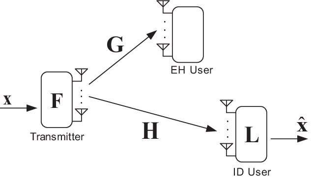
With these assumptions, the estimated signal $\hat{\mbox{$\bf x$}}\in\mathbb{C}^{N_{S}\times 1}$ at the ID user can be modeled by

where $\mbox{$\bf n$}\in\mathbb{C}^{N_{\text{ID}}\times 1}$ indicates the receiver noise with $\mbox{$\bf n$}\sim\mathcal{CN}(\mathbf{0},\mbox{$\bf I$}_{N_{\text{ID}}})$, $\mbox{$\bf L$}\in\mathbb{C}^{N_{S}\times N_{\text{ID}}}$ represents the linear receiver at the ID user, and $\mbox{$\bf F$}\in\mathbb{C}^{N_{T}\times N_{S}}$ is the linear precoder at the transmitter, which is subject to the power constraint $\text{Tr}(\mbox{$\bf F$}\mbox{$\bf F$}^{H})\leq P_{T}$. Then, the estimation error at the ID user can be defined as $\mbox{$\bf e$}=\gamma^{-1}\hat{\mbox{$\bf x$}}-\mbox{$\bf x$}$ and the resulting weighted sum-MSE is given by $\text{MSE}=\text{Tr}(\mbox{$\bf W$}\mathcal{E}[\mbox{$\bf e$}\mbox{$\bf e$}^{H}])$. Here, the scaling parameter $\gamma^{-1}$ plays a role of automatic gain control [12] which helps simplifying the derivation and $\bf W$ stands for a real diagonal weight matrix. Note that without consideration of the EH user, the MMSE optimum transmitter design which we denote by $\mbox{$\bf F$}_{\text{ID}}$ is well investigated in literature [8].

In the meantime, the total harvested energy at the EH receiver, defined by $Q$, can be expressed as

where $\delta$ is a constant accounting for the harvesting efficiency and we assume $\delta=1$ for simplicity unless stated otherwise. Let $\sqrt{g_{1}}$ and $\mbox{$\bf v$}_{g,1}\in\mathbb{C}^{N_{T}\times 1}$ denote the largest singular value of $\bf G$ and the corresponding right singular vector, respectively. Then, it is known that the energy beamformer $\mbox{$\bf F$}_{\text{EH}}=\sqrt{P_{T}}[\mbox{$\bf v$}_{g,1}~\mathbf{0}_{N_{T}\times(N_{S}-1)}]$ achieves the maximum energy $E_{\max}=P_{T}g_{1}$ [3] [7]. and we denote the achievable sum-MSE with this beamformer by $M_{EH}$. Meanwhile, the sum-MSE and the energy attainable by the MMSE precoder $\mbox{$\bf F$}_{\text{ID}}$ are denoted by $M_{\min}$ and $E_{\text{ID}}$, respectively.

Now, consider the case where both the EH and ID users co-exist. Then, the achievable MSE-energy region is

and each boundary point of $\mathcal{R}_{M,E}$ can be obtained by solving the following SWIPT-WMMSE optimization problem

where $E_{\text{ID}}\leq\bar{E}\leq E_{\max}$. This problem is convex over the transmitter (receiver) when the receiver (transmitter) and $\gamma$ are given, and strictly quasi-convex with respect to $\gamma$ when both $\bf F$ and $\bf L$ are given. However, it is generally non-convex on $\{\gamma,\mbox{$\bf F$},\mbox{$\bf L$}\}$. Our goal of the paper is to find efficient solutions to problem (3) and identify the best possible MSE-energy region $\mathcal{R}_{M,E}$.

In this section, we solve the problem (3) based on the Karush-Kuhn Tucker (KKT) conditions. First, we propose the optimum precoder structure in terms of the WMMSE, and then suggest alternative optimization process between the transmitter and the ID receiver. Several interesting observations will also be made when the ID user is equipped with a single antenna.

Using the expression of $\bf e$ and the assumptions made in the previous section, we formulate the Lagrangian as

Then, the following KKT conditions provide necessary conditions for optimality:

where $\bar{\lambda}\triangleq\lambda\gamma^{2}$, $\bar{\mu}\triangleq\mu\gamma^{2}$, and equations (5)-(7) are derived from the zero gradient conditions by using some rules of differentiation [13] and (9) and (10) come from the complement slackness conditions.

Now, let us define two matrices that will be used for our derivations as

Here, $\bf Y$ is a positive definite matrix, but $\bf Z$ is in general positive indefinite which makes the analysis challenging. Based on these results, each of the transmitter and the receiver can be optimized separately as in the following theorems.

In this section, we provide several interesting observations by comparing the numerical performance of the two MIMO BC SWIPT design criteria: WMMSE and the information rate [7]. Key system parameters are summarized in Table I. Throughout our simulation, the channels are generated from Rayleigh fading pathloss model, $\mbox{$\bf H$}=d_{h}^{-3/2}\widetilde{\mbox{$\bf H$}}$ and $\mbox{$\bf G$}=d_{g}^{-3/2}\widetilde{\mbox{$\bf G$}}$ where each element of $\widetilde{\mbox{$\bf H$}}$ and $\widetilde{\mbox{$\bf G$}}$ is drawn from the i.i.d. CSCG normal distribution according to the MATLAB code with the seed number $\theta$ as in Table I. Also, we set $N_{T}=N_{S}=N_{\text{ID}}=N_{\text{EH}}=4$ and $d_{h}=d_{g}=10$(m) for the ease of the presentation. Let us assume that $P_{T}=20$ dBm ($100mW$). Then, since the noise power is $-100$ dBm/Hz $\times$ $100$MHz=$1\mu W$, the per-antenna SNR at the ID user becomes $20-30-(-30)=20$ dB, which is equivalent to the standard signal model with $P_{T}=10^{5}$ in (1). Thus, $1$ energy unit at the EH user in (2) amounts to $1\mu W$ in our simulation setting.

Figure 2-(a) and 2-(b) illustrate the convergence trends of the proposed scheme with $P_{T}=100$mW in terms of both the sum-MSE and the information rate with weight matrices $\mbox{$\bf W$}=\mbox{$\bf I$}_{4}$ and $\mbox{$\bf W$}=\mathbf{\Lambda}_{H}$, respectively, where $\mathbf{\Lambda}_{H}$ indicates the eigenvalue matrix of $\mbox{$\bf H$}^{H}\mbox{$\bf H$}$. In each iteration, the sum-MSE ($M$) and the rate ($R$) are computed from $M=\text{Tr}(\mbox{$\bf W$}(\mbox{$\bf F$}^{H}\mbox{$\bf H$}^{H}\mbox{$\bf H$}\mbox{$\bf F$}+\mbox{$\bf I$}_{N_{T}})^{-1})$ and $R=\log|\mbox{$\bf F$}^{H}\mbox{$\bf H$}^{H}\mbox{$\bf H$}\mbox{$\bf F$}+\mbox{$\bf I$}_{N_{T}}|$ under the assumption that the ID user employs the MMSE receiver (13) and the maximum likelihood receiver, respectively. Due to the non-convexity of problem (3), the resulting performance depends on the number of initial points and iterations, especially when the weight matrix is non-identity. Nevertheless, it is seen that $20$ random initial points and $10$ number of iterations seem to be sufficient to achieve the converged performance for our scheme. It is somewhat natural that the proposed MMSE scheme obtains improved MSE performance over the “SWIPT-Rate” scheme [7]. However, it is particularly interesting to observe that our solution achieves the optimum rate as well when the weight factors are properly chosen, which implies that the rate maximizing precoder design can be regarded as a special case of our WMMSE design¹¹ 1 Similar observation has been made in point-to-point MIMO systems without energy transfer [8]. Extensive computer simulations confirm that $\mbox{$\bf W$}=\mathbf{\Lambda}_{H}$ is the best choice for maximizing the rate, but rigorous proof remains open.

Figures 3 and 4 illustrate the boundary points of the achievable MSE-energy and rate-energy regions, respectively. 20 random initial points are used for the proposed SWIPT-WMMSE scheme. It is shown that our solution achieves the outstanding MSE-energy region compared to the SWIPT-Rate scheme [7], which leads to the BER performance improvement as is shown later. In addition, Figure 4 shows that when $\mbox{$\bf W$}=\mathbf{\Lambda}_{H}$, the WMMSE precoder achieves almost every boundary points of the optimal rate-energy region; thus, confirming the previous observation made in Figure 2. We would like to note that although here we presented simulations results for a sample channel ($\theta=11$), the trend does not change for all channel realizations.

Figure 5 compares the uncoded BER performance of the two MIMO BC SWIPT systems with 4QAM. We averaged over $10^{5}$ random channel realizations and set $\bar{E}=E_{\max}/2$ in each realization so that the EH user harvests at least $50$% of the maximum energy allowed for a given channel. The figure shows that the proposed MMSE scheme with $\mbox{$\bf W$}=\mbox{$\bf I$}_{4}$ obtains approximately $5$ dB gain over the SWIPT-Rate scheme. This is because the rate-based precoder allocates more resource to the stronger sub-channel, while the MMSE precoder neutralizes the channel gains across sub-channels. On the contrary, for the same reason, the rate-based design may exhibit better error performance when the transmitter adopts sufficiently strong channel codes. The proposed WMMSE precoder will softly bridge two extreme cases by adjusting the weight matrix $\bf W$.

In this paper, we investigated efficient linear transceiver designs for MIMO BC SWIPT systems which minimizes the weighted sum-MSE of the ID-user while satisfying the energy harvesting constraint of the EH-user. First, we identified the optimal precoder structure as a closed-form solution that can be obtained by simple bisection methods. Then, it was shown that the derived precoder achieves the maximum SNR at the ID user with reduced complexity when the ID user has a single antenna. Second, we suggested alternative updating process to obtain the joint WMMSE solution with the ID receiver. Although the problem is non-convex, it is observed from simulation results that our solution with multiple initial points approaches the best possible MSE-energy tradeoff region. It was also interesting to observe that the proposed WMMSE precoder with $\mbox{$\bf W$}=\mathbf{\Lambda}_{H}$ achieves almost every boundary points of the optimal rate-energy region.

This work was supported in part by FP7 project PHYLAWS (EU FP7-ICT 317562).

References

- [1] P. Grover and A. Sahai, “Shannon meets Tesla: Wireless information and power transfer,” in Proc. IEEE International Symposium on Information Theory (ISIT’10), pp. 2363–2367, June 2010.
- [2] L. R. Varshney, “Transporting information and energy simultaneously,” in Proc. IEEE International Symposium on Information Theory (ISIT’08), pp. 1612–1616, July 2008.
- [3] J. Park and B. Clerckx, “Joint wireless information and energy transfer in a two-user MIMO interference channel,” IEEE Trans. Wireless Commun., vol. 8, pp. 4210–4221, August 2013.
- [4] A. A. Nasir, X. Zhou, S. Durrani, and R. A. Kennedy, “Relaying protocols for wireless energy harvesting and information processing,” vol. Available:http://arxiv.org/abs/1212.5406, 2012.
- [5] J. Xu, L. Liu, and R. Zhang, “Multiuser MISO Beamforming for Simultaneous Wireless Information and Power Transfer,” in Proc. IEEE International Conference on Acoustics, Speech, and Signal Processing (ICASSP), 2013.
- [6] H. Son and B. Clerckx, “Joint beamforming design for multi-user wireless information and power transfer,” to appear in IEEE Trans. Wireless Commun.
- [7] R. Zhang and C. K. Ho, “MIMO broadcasting for simultaneous wireless information and power transfer,” IEEE Trans. Wireless Commun., vol. 12, pp. 1989–2001, May 2013.
- [8] H. Sampath, P. Stoica, and A. Paulraj, “Generalized linear precoder and decoder design for MIMO channels using the weighted MMSE criterion,” IEEE Trans. on Commun., vol. 49, pp. 2198–2206, Dec. 2001.
- [9] D. P. Palomar, J. M. Cioffi, and M. A. Lagunas, “Joint Tx-Rx beamforming design for multicarrier MIMO channels: a unified framework for convex optimization,” IEEE Trans. Signal Process., vol. 51, pp. 2381–2401, September 2003.
- [10] C. Song, K.-J. Lee, and I. Lee, “MMSE based transceiver designs in closed-loop non-regenerative MIMO relaying systems,” IEEE Trans. Wireless Commun., vol. 9, pp. 2310–2319, July 2010.
- [11] M. Joham, W. Utschick, and J. A. Nossek, “Linear transmit processing in MIMO communications systems,” IEEE Trans. Signal Process., vol. 53, pp. 2700–2712, August 2005.
- [12] J. Joung and Y. H. Lee, “Regularized channel diagonalization for multiuser MIMO downlink using a modified MMSE criterion,” IEEE Trans. Sig. Process., vol. 55, pp. 1573–1579, Apr. 2007.
- [13] A. Hjørungnes and D. Gesbert, “Complex-valued matrix differentialtion: Techniques and key results,” IEEE Trans. Signal Process., vol. 55, pp. 2740–2746, Jun. 2007.
- [14] G. H. Golub and C. F. V. Loan, Matrix Computations. Third Edition, The Johns Hopkins University Press, Baltimore and London, 1996.