Direct Experimental Determination of Spectral Densities of Molecular Complexes
Abstract
Determining the spectral density of a molecular system immersed in a proteomic scaffold and in contact to a solvent is a fundamental challenge in the coarse-grained description of, e.g., electron and energy transfer dynamics. Once the spectral density is characterized, all the time scales are captured and no artificial separation between fast and slow processes need be invoked. Based on the fluorescence Stokes shift function, we utilize a simple and robust strategy to extract the spectral density of a number of molecular complexes from available experimental data. Specifically, we show that experimental data for dye molecules in several solvents, amino acid proteins in water, and some photochemical systems (e.g., rhodopsin and green fluorescence proteins), are well described by a three-parameter family of sub-Ohmic spectral densities that are characterized by a fast initial Gaussian-like decay followed by a slow algebraic-like decay rate at long times.
I Introduction
The accurate description and quantification of solvent effects on the electronic dynamics of molecular systems are of great importance to reactions,[1] various spectroscopies[2, 3] and to charge and electronic energy transfer[4]. In these cases solvent and, as we discuss below, intra- and inter-molecular vibrations play a dual role: the solvent screens the electronic dynamics due to the spectral broadening but at the same time provides the energy to initiate chemical reactions and to stabilize products once reactions have occurred[2].
Despite its relevance, and due to the number of degrees of freedom involved in the description of such systems, the role of the solvent and vibrations (induced, e.g., by proteomic scaffolds or nuclear motion) are effectively treated by means of statistical approaches [5, 6, 2, 3, 7, 4, 8, 9, 10, 11]. In these approaches, the fundamental ingredient is the spectral density, which models the effect of the solvent and vibrations. Once the spectral density is characterized, all the time scales involved in the dynamics are captured and there is no need for an artificial separation between fast and slow processes. Moreover, having the exact spectral density for a particular system allows for the inclusion of quantum correlations (see below) in the calculation of solvated processes (e.g., electron transfer)[5, 6, 2].
Being a key element in the effective description of the system-bath coupling, it is clear that the equilibrium and non-equilibrium features of the system dynamics are heavily determined by the spectral density . In order to gain information about it suffices, in accord with the fluctuation dissipation theorem (see below)[12], to measure either the non-equilibrium relaxation or the equilibrium fluctuations. This connection lead Fleming and Cho[2] to suggest a spin-boson approach that allows extracting the spectral density from the Stokes shift response-function. Despite the available experimental data for various systems, e.g., dye molecules[13, 14], amino acid proteins[15], or photochemical complexes[16, 17], and the clear advantage of extracting directly from experiment, this robust strategy remains unexplored. Only recently, based on quantum-classical simulations of the non-equilibrium features, has this connection been used for light-harvesting systems,[18] leading to a calculated highly structured spectral density for FMO, which is in good agreement with the spectral density inferred from the absorption spectrum[19].
We show below that, based on experimental data for the Stokes shift response-function, the initial fast relaxation followed by a slow relaxation, typical in available data[13, 15, 16, 17], can be well characterized by the three-parameter family of sub-Ohmic spectral densities,[20, 21, 22] whose features are discussed below. Sub-Ohmic spectral densities are typical for noisy process in solid state devices at low temperatures such as superconducting qubits[23] and quantum dots[24]. They also appear in the context of ultra-slow glass dynamics[25], quantum impurity systems[26], nanomechanical oscillators[27] and fractal environments such as porous and viscoelastic media[20] and reservoirs with chaotic dynamics[21]. An important feature of the parametric family of sub-Ohmic spectral densities is the fact that, for a broad class of members, incoherent relaxation does not occur. Hence, coherent processes can have long lifetimes, even in the regime of strong coupling to the environment[22].
This paper is organized as follows: the formalism that relates the Stokes shift response function to is described in Sect. II. Note is made of the primary requirement, adherence to linear response theory, and justification cited for the applicability of linear response for the cases studied. Section III discusses attributes of the sub-ohmic spectral density, extracted in Sect. IV from experimental data. Additional aspects of this approach are the subject of Sect. V and the Appendices. Section VI contains a brief summary.
II The Stokes Shift Response-Function
The Stokes shift response function (or time-dependent solvation correlation function) describes the solvent response to a sudden change in the charge distribution of a solute molecule,[14, 28, 29, 30] and has been measured over different time scales and for a variety of polar solvents (cf. Refs. 14, 28, 29, 30 and references therein). We briefly rederive the relationship between the fluorescence Stokes shift and the spectral density in order to expose the underlying assumptions. The essential argument follows that in Ref. 2.

In typical Stokes shift experiments, a chromophore solute in a polar solvent is first excited by a pump pulse, and the time-dependent fluorescence spectrum of the solute is then recorded[14] (see Fig. 1). In terms of experimental accessible quantities, the fluorescence Stokes shift function is defined as[2]
| (1) |
where is the non-equilibrium energy difference between the excited state and the ground state and is proportional to the time dependence of a characteristic fluorescence frequency. The goal is then to relate the non-equilibrium relaxation encoded in with equilibrium fluctuations of the energy difference and then extract the spectral density. In doing so, let us a consider a two-electronic state system, with electronic transition frequency , coupled to a thermal bath via the interaction term , and to a radiation field via the dipole moment , so that the Hamiltonian is described by
| (2) |
Here ’s are the Pauli matrices and and denote the bath and system coordinates, respectively.
Following Ref. 2, we use the Heisenberg picture and split the interaction term into an average and a fluctuating part, . As is customary, in order to have an effective description of the coupling to the bath, one assumes that behaves as a random variable and that it is characterized by its symmetrized, , and anti-symmetrized correlation functions[2, 3], . For convenience below we note that in accord with Kubo’s formula, the linear response of the system to the fluctuating perturbation is defined as the mean value of the commutator , i.e., in terms of the anti-symmetrized correlation function . The spectral density , the central element in the present discussion, is then defined in terms of the Fourier transform of the response function, so that[2]
| (3) |
where
For the Stokes shift function, one assumes that the energy difference operator can be divided into two contributions where is the average transition energy. Linear response theory then allows the fluctuation due to the perturbation to be generally written as an integral over the response function. The normalized fluorescence Stokes shift function then becomes Given the relationship between the spectral density and the response function [Eq. 3], the fluorescence Stokes shift function can be rewritten in terms of the spectral density as
| (4) |
where the normalization constant is identical to the solvent reorganization energy. It can be obtained experimentally from , or by any alternatively available route.
By inverting Eq. 4, the spectral density is obtained directly as
| (5) |
This expression allows us, by means of a simple Fourier transform, to obtain the spectral density for a given physicochemical system from a measured . The so obtained is as accurate as is the observed , and provides a direct means of understanding features of in terms of the underlying . Further, improvements in the measured lead naturally to improved values for . Note that alternative ways to estimate the spectral density rely on fitting procedures based on the absorption and fluorescence spectra, which are obtained from the line shape function [e.g., see Ref. 3]. Thus, whereas alternative approaches provide only indirect information about the spectral density, Eq. 5 offers a direct route between and the measured data.
Before proceeding further, some comments are in order. (i) For an harmonic bath, the right hand side of Eq. 4 defines the damping kernel discussed elsewhere[10] and, within the spin-boson case, defines . (ii) Note that the Hamiltonian in Eq. 2 implicitly assumes that the coupling to the bath describes the interaction with the solvent and the intra- and inter-nuclear co-ordinates, i.e., that the Franck-Condon progressions include all the coupled modes. (iii) The present analysis is based on the linear response approximation which is expected to be accurate for chromophores with relative large size and modest charge variations[31], such as those treated here. It fails in significantly different types of systems, e.g., small solutes showing sizeable variations in atomic charges[31]. Thus, we expect that an effective description based on Eq. 4 is sensible for the systems discussed below. (iv) Equation (5) makes clear that the higher the resolution of the observed , the more detail obtainable for .
Below we develop this approach for a number of examples.
III Dye Molecules: Motivating the Sub-Ohmic Spectral Density
In Ref. 13, the Stokes shift response function was measured for Coumarin 343, with water as a solvent. The experimental results were well characterized by three terms, a fast Gaussian decay and two slow exponential decays,
| (6) |
with , ps-1, , ps, and ps. The time dependence of is depicted in Fig. 2. This figure shows a universal behavior present in many solvated experiments in water [and, in general, in polar solvents such as acetonitrile or methyl chloride (cf. Ref. 2 and references therein)][13, 15, 31]: an ultrafast Gaussian-type decay followed by an exponential-type slow component. In this context, the ultrafast component is usually associated with librational (rotational) motions of water molecules (or molecules of light molecular solvents) while the slow component, due to the mass of the oxygen atom, is associated with translational motion[13]. In the presence of a proteomic scaffold, the scaffold vibrations can also contribute to the translational motion of water molecules[31] and therefore contribute to the slow decaying component.

Given Eqs. (5) and (6), the Stokes shift response function, the spectral density follows straightforwardly from Eq. 5 and, for this case, would be given by
| (7) | ||||
Although the spectral density in Eq. 7 or the Stokes function in Eq. 6 fit the experimental data, they contain six free parameters that are essentially artificial because one would expect, from the character of the data, that only two gross time scales would suffice. Hence, our proposal is to numerically evaluate Eq. 5 using the observed and extract . Prior to doing so, we recognize in Fig. 2 a typical behavior well known in the context of open quantum systems[20, 21]: the one induced by sub-Ohmic spectral densities. Hence, we first describe below the main properties of this parametric family of spectral densities, and then make a connection with results for Coumarin 343, amino acid proteins[15], bovine rhodopsin[16] and green fluorescence proteins such as mPlum, mRFP and mRaspberry[17]. (The Appendix deals with some misunderstandings[32] that suggest that sub-Ohmic spectral densities are not acceptable.)
III.1 Sub-Ohmic spectral densities
An initial fast relaxation followed by a slow relaxation is common in many solvated measurements. This behavior is familiar in noisy processes in superconducting qubits[23] and quantum dots[24], ultra slow glass dynamics[25], quantum impurity systems[26], nanomechanical oscillators[27] and fractal environments[20] and is often described in terms of the parametric family of sub-Ohmic spectral densities described by
| (8) |
with . The Ohmic spectral density follows from the case of . Here, is the dimensionless coupling-to-the-environment constant, is a cutoff frequency and is an auxiliary phononic scale frequency, not present in the Ohmic case, such that the relevant coupling constant is . The parameter values are determined by the nature of the environment and its interaction with the system. 11 1 Note that in other contexts[22], the spectral density is defined without the factor in Eq. 3 and therefore for the sub-Ohmic case .
For the sub-Ohmic case, the Stokes shift function is
| (9) |
where we note that only two time scales are present. In the short time regime, , , which resembles the functional form of a Gaussian decay at short times. In the long time regime, , , so that the long time decay is algebraic, . In this case, the reorganization energy, introduced in Eq. 4 reads
| (10) |
where denotes the gamma function of [34]. A full characterization of the dynamics and spectral quantities, requires consideration of other quantities, such as the Huang-Rhys factor, discussed in the Appendix.
For the sake of completeness, we present explicit results based on the sub-Ohmic spectral density Eq. 8 for the relevant quantities in echo spectroscopies. Assuming that obeys a Gaussian statistics, it is possible to express the third-order non-linear signals in terms of the line shape function ,
| (11) |
where and are the symmetrized and anti-symmetrized correlation function, defined above[2, 3, 35]. The real part of describes the spectral broadening, whereas the imaginary part is related to the fluorescence Stokes shift [cf. Eq. 4].
In terms of the spectral density, the line shape function in Eq. 11 can be expressed as[2, 3]
| (12) |
where we can identify the time-derivative of the second term of the first line with the Stokes shift function and the second line contains the effects of the thermal environment and zero-point fluctuations. For the particular case of the sub-Ohmic spectral densities, we have
| (13) |
with and is the generalized Riemann’s zeta function 22 2 For all values of expect , see Eq. 9.512 in Ref. 34, .. Once the line shape function is known, the fluorescence and absorption spectra can be obtained.[3]
III.1.1 Cumarin 343
In order to explore to what extent the sub-Ohmic description is quantitative for the Cumarin 343 example in Fig. 2, we fit the experimental data from Ref. 13 to a sub-Ohmic spectral density with ps-1 and . As shown in Fig. 2, the sub-Ohmic spectral density, with only two parameters, correctly describes the fast initial decay and the subsequent slow relaxation observed in the experiment and fitted to in Eq. 6. Also shown for comparison, is the single exponential decaying Stokes shift function derived for an Ohmic spectral density, , which clearly fails to describe the experimental behavior.
In the following, we consider the nature of for more complex systems, such as amino acid proteins and photochemical systems.
IV Analyzed Spectral Densities
IV.1 Amino Acid Proteins
For this particular case, as well as the case of pigment aggregates, an ideal probe for studying protein dynamics and electrostatics should be sensitive to its environment and should be able to be incorporated, site-specifically, throughout any protein of interest[15]. In Ref. 15, Adalan, an environment-sensitive fluorescent amino acid, was synthesized and site-specifically incorporated into proteins by both nonsense suppression and solid-phase synthesis. In particular, Adalan was used to probe the electrostatic character of the B1 domain of streptococcal protein G (GB1) at multiple sites using time-resolved fluorescence. Fig. 3 shows the experimental results for the dynamic Stokes shifts for the Phe30 (buried in the protein), Leu7 (buried in the protein) and Trp43 (partially exposed in the protein) mutants, extracted from Ref. 15 and our fit using a sub-Ohmic spectral density. It is clear that the short as well as the long time dynamics are extremely well characterize by Stokes shift function in Eq. 9, which is induced by the sub-Ohmic spectral density.

Understanding the origin of the particular parameter values from the fitting procedure, which vary considerably for the three cases (see figure caption, Fig. 2) requires a deep analysis of the interaction between the pigments, the proteomic scaffold and the solvent. However, an immediate consequence of our effective description is that it simplifies the calculation of cross-grained quantities such as line shape functions described above (see III.1) and excitation energy transfer rates [cf. Chap. 9 in Ref. 4] and provides a starting point for analysis of the features of the spectral density.
IV.2 Photochemical Systems
Recently, there has been a great interest in the dynamics of photochemical systems [16, 37, 38, 39, 40, 6, 17, 7, 4, 8, 10, 11]. In particular, two cases have been extensively investigated: (i) the cis/trans isomerization of rhodopsin,[16, 37, 38, 39, 40] and (ii) the energy transfer processes in natural light-harvesting systems.[6, 17, 7, 4, 8, 10, 11] Below, we explore the extent to which the sub-Ohmic spectral density describes available experimental data for the dynamic Stokes shift of these systems.
IV.2.1 Rhodopsin
Rhodopsin is an excellent molecular switch which converts light signals to the electrical response of the photoreceptor cells,[16] and which has been extensively studied.[16, 37, 38] In Ref. 16, the Stokes shift function was measured for the case of bovine rhodopsin at various wavelengths. As shown in Fig. 4, the description based on the sub-Ohmic spectral density is highly accurate in all cases, which correspond to different excitation wavelengths . We note that the spectral density needs to be recalculated for each since each wavelength excites different constituents of the molecular complex. As a consequence, each wavelength induces different behavior of the vibrational modes and solvent response.
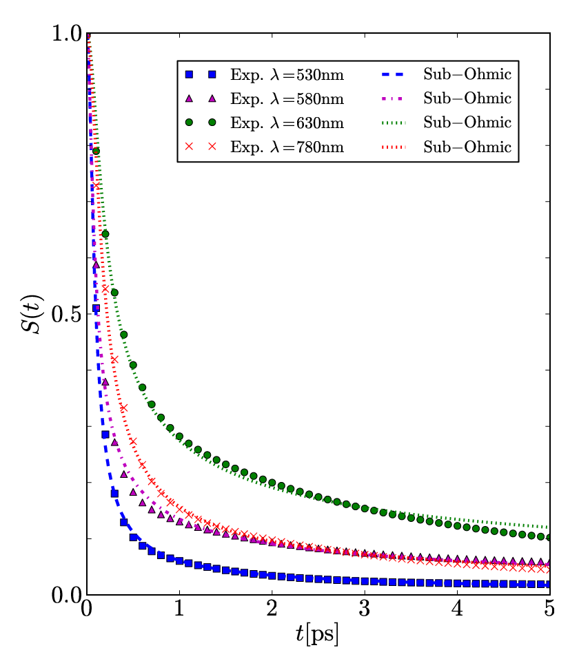
Note that this representation allows for a dramatic simplification of calculations needed to, for example, explore the time evolution of rhodopsin since the effect of all Raman modes can now be effectively condensed in a sub-Ohmic spectral density.
IV.2.2 Green Fluorescent Protein
Green Fluorescent Proteins (GFPs) are thought to be ideal candidates for measurements of the dynamic Stokes shift because the chromophore is both intrinsic to the protein and structurally well characterized[17]. This feature was exploited in Ref. 17 to measure the dynamic Stokes shift function in variants of GFP such as mPlum, mRFP and mRaspberry at different pH levels. The experimental results available from Ref. 17 are those from a fitting procedure to a log-normal line-shape with, due to the weak solvation, an added baseline parameter. Hence, in order to properly describe the based on the sub-Ohmic spectral density, we also introduce a baseline contribution , so that for this case is , with given by Eq. 9.
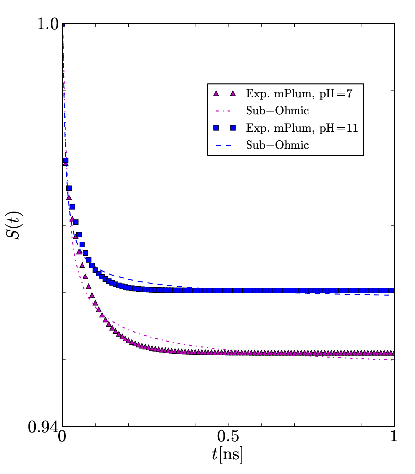
In Fig. 5, we depict the experimental results and their characterization based on the sub-Ohmic spectral density for mPlum at pH 7 and pH 11. As in previous cases, the accuracy of the description is very good. For the case of mRFP ( ps-1 and ) and mRaspberry ( ps-1 and ) in pH 7 buffer (not shown), the description is also very accurate, with no need for an additional baseline contribution.
V Additional Remarks
We have discussed an experimentally accessible way to directly determine the spectral densities of molecular complexes, which is also applicable to systems in solid state physics such as quantum dots. Below, we discuss some technical points related to this formulation, and to semiclassical approaches aimed at calculating .
Classical vs. Quantum Correlations—Due to the sheer complexity of ab initio calculations of the dynamics of large physicochemical systems [cf. Ref. 6, 31, 18], computational studies of usually invoke classical treatments of the nuclear dynamics. Thus, in the classical limit, since the spectral distribution of fluctuations is far less than , the response function is directly related to the classical correlation function where the average is taken over classical phase space and is a classical variable. Hence,
| (14) |
which is a formal expression of the classical Onsager regression hypothesis.
It is important to note that, formally, the regression hypothesis fails in the quantum regime[41] and in the case of Markovian dynamics, violates the Kubo-Martin-Schwinger[42, 43] principle of detailed balance[44]. That is,[2] in the classical limit the temperature is the only parameter determining the fluctuation-dissipation relation (cf. Ref35 and references therein), whereas in the quantum case, the fluctuation-dissipation relation requires complete knowledge of the spectral distribution of the fluctuation[45]., i.e., . The present approach is based on experimental data, since it has the advantage of making no reference to the classical or quantum nature of the correlations, it just makes use of the general quantum formulation. The “quantumness” of the correlations then emerges directly from the experimental data. Thus, having the possibility of extracting the spectral density directly from experimental data is not only of practical importance, but also is significant from a fundamental viewpoint.
VI Summary
The results of this work show clearly that sub-Ohmic spectral densities provide an excellent description of the spectral densities associated with an impressive number of large solvated systems, and that such spectral densities can be directly extracted, within the spin-boson model, from the experimental Stokes shift response function . Higher resolution may yield more detailed ), but the smooth underlying sub-Ohmic spectral density structure is expected to persist. These results, plus the extensive literature on sub-Ohmic spectral densities that describe their physical consequences and characteristics, encourage greater theoretical and experimental studies on both the Stokes shift response function and on the interpretation of the observed sub-Ohmic parameters in physicochemical systems.
One further note is in order. Our recent work on the theory of one-photon phase control of molecular systems[46, 39, 40], shows that the sub-Ohmic character could assist the one-photon phase control, and effect that was motivated by experiments at low[37] and high[38] field intensities. As a consequence, the broad range of systems displaying sub-Ohmic behavior is encouraging for one-photon phase control of such systems.
Acknowledgements.
Comments by G. D. Scholes and references suggested by B. E. Cohen are gratefully acknowledged. This work was supported by the US Air Force Office of Scientific Research under contract number FA9550-13-1-0005, by the Comité para el Desarrollo de la Investigación –CODI– of Universidad de Antioquia, Colombia under contract number E01651 and under the Estrategia de Sostenibilidad 2013-2014, by the Departamento Administrativo de Ciencia, Tecnología e Innovación –COLCIENCIAS– of Colombia under the grant number 111556934912.VII Appendix
It is illustrative to examine some previous considerations[32] about the zero phonon line in absorption spectra of chromophores in solid structure. There, it was argued that physically relevant spectral densities should converge to zero as the frequency approaches zero. For the widely used family of spectral densities of the form[20, 21] , this would require , ruling out the sub-Ohmic (), Ohmic () and super Ohmic () spectral densities. However, such as an argument arises from an incomplete understanding of the quantum fluctuation-dissipation theorem[12] (see e.g. Ref. 35 or Chap. 6 in Ref. 21) and the homodyne nature of the spectrum measurement-process via absorption[47]. Hence, it is pertinent to comment on these issues.
The Quantum Fluctuation-Dissipation Theorem. The classical fluctuation-dissipation theorem formulated in 1928 by Nyquist[48], and experimentally verified by Johnson[49], states that a resistor , in response to the inherent fluctuations in maintaining a Boltzmann distribution of the canonical variables in an electric circuit, develops a current voltage across its ends. The Fourier-transformed two-point-correlation-function of the induced current, , is given by[47]
| (15) |
Motivated by the work of Planck on the quantized spectrum of the blackbody radiation, in the last paragraph of his 1928 paper, Nyquist considered the case when , which he suggested should be equivalent to taking .
A formal treatment of the quantum results of Nyquist was provided by Callen and Welton,[12] who showed that the correct correlation function reads
| (16) |
where is equivalent to the susceptibility, which for the case of a Markovian Ohmic resistor corresponds to , i.e., frequency independent dissipation. Thus, by contrast to Nyquist’s original suggestion, at low temperature (), the grows linearly with due to the zero point fluctuations , i.e. due to the quantum noise. Most importantly, the quantum noise has an associated non-zero susceptibility and therefore one expects a finite width to the zero phonon line (ZPL). However, as the authors in Ref. 32 correctly noted, for a multitude of molecular systems there is no experimental evidence of such a finite width for the ZPL at K. This observation lead them to argue, incorrectly, that the ZPL profile has zero width at 0 K.
The Homodyne Nature of the Spectrum Measurement-Process by Absorption. The fact that the experimental data does not provide any evidence of a finite width of the ZPL at K is analogous to the fact that the detected blackbody-radiation-spectrum is well described by the Planck distribution with no contribution of the linear term in Eq. 16. The reason for this is that we cannot detect the zero point energy contribution to the spectrum when we use experimental homodyne schemes that are based on the absorption of photons from a radiation field[47]. Specifically, in homodyne absorption measurements, what is measured is the normal product of the creation and annihilation operators of the field (see, e.g., Chap. 8 in Ref. 47), and hence there is no zero point contribution. However, this does not mean that the effect of the zero point energy is not accessible experimentally; it was indeed measured[50] by means of heterodyne detection at 1.6 and 4.2 K. However, at high temperature , the main contribution comes from the Planck distribution of the thermal bath, and the spectral lines are expected to have a finite width.
On the Huang-Rhys factor for Sub-Ohmic Spectral Densities. The Huang-Rhys factor can be seen as a measure of the effective mass of the environment.[51, 21] For the case of the sub-Ohmic spectral density introduced in Eq. 8 it is defined as
| (17) |
In the context of open quantum systems[21], the divergence of this integral is known to lead to orthogonality catastrophe, a concept we will not discuss here. In the super-Ohmic case , the integral in infrared-convergent and, in the case of a two-level system, is an indication of possible elastic tunneling without dynamical involvement of the bath. In the sub-Ohmic case , the integral is infrared-divergent, which means that the low frequency modes must be treated non-adiabatically, a procedure that can be found in Ref. 21, Sec. 20.2.
References
- [1] P. Hänggi, P. Talkner, and M. Borkovec, Rev. Mod. Phys. 62, 251 (1990).
- [2] G. R. Fleming and M. Cho, Ann. Rev. Phys. Chem. 47, 109 (1996), http://www.annualreviews.org/doi/pdf/10.1146/annurev.physchem.47.1.109 .
- [3] S. Mukamel, Principles of Nonlinear Optical Spectroscopy (Oxford University Press, New York, 1999).
- [4] V. May and O. Kühn, Charge and energy transfer dynamics in molecular systems, 3rd ed. (Wiley-VCH, Weinheim, 2011).
- [5] J. S. Bader, R. A. Kuharski, and D. Chandler, The Journal of Chemical Physics 93, 230 (1990).
- [6] A. Warshel and W. W. Parson, Annual Review of Physical Chemistry 42, 279 (1991), pMID: 1747189, http://www.annualreviews.org/doi/pdf/10.1146/annurev.pc.42.100191.001431 .
- [7] A. Ishizaki, T. R. Calhoun, G. S. Schlau-Cohen, and G. R. Fleming, Phys. Chem. Chem. Phys. 12, 7319 (2010).
- [8] L. A. Pachón and P. Brumer, J. Phys. Chem. Lett. 2, 2728 (2011), arXiv:1107.0322v2 .
- [9] J. Moix, J. Wu, P. Huo, D. Coker, and J. Cao, J. Phys. Chem. Lett. 2, 3045 (2011), http://pubs.acs.org/doi/pdf/10.1021/jz201259v .
- [10] L. A. Pachón and P. Brumer, Phys. Chem. Chem. Phys. 14, 10094 (2012), arXiv:1203.3978 .
- [11] A. W. Chin, J. Prior, R. Rosenbach, F. Caycedo-Soler, S. F. Huelga, and M. B. Plenio, Nat. Phys. 9, 113 (2013).
- [12] H. B. Callen and T. A. Welton, Phys. Rev. 83, 34 (1951).
- [13] R. Jimenez, P. V. Fleming, G. R.and Kumar, and M. Maroncelli, Nature 369, 471 (1994).
- [14] C.-P. Hsu, X. Song, and R. A. Marcus, J. Phys. Chem. B 101, 2546 (1997).
- [15] B. E. Cohen, T. B. McAnaney, E. S. Park, Y. N. Jan, S. G. Boxer, and L. Y. Jan, Science 296, 1700 (2002).
- [16] H. Kandori, Y. Furutani, S. Nishimura, Y. Shichida, H. Chosrowjan, Y. Shibata, and N. Mataga, Chemical Physics Letters 334, 271 (2001).
- [17] P. Abbyad, W. Childs, X. Shi, and S. G. Boxer, Proceedings of the National Academy of Sciences 104, 20189 (2007), http://www.pnas.org/content/104/51/20189.full.pdf+html .
- [18] S. Valleau, A. Eisfeld, and A. Aspuru-Guzik, The Journal of Chemical Physics 137, 224103 (2012).
- [19] J. Adolphs and T. Renger, Biophys. J. 91, 2778 (2006).
- [20] A. J. Leggett, S. Chakravarty, A. T. Dorsey, M. P. A. Fisher, A. Garg, and W. Zwerger, Rev. Mod. Phys. 59, 1 (1987).
- [21] U. Weiss, Quantum Dissipative Systems, 4th ed. (World Scientific, Singapore, 2012).
- [22] D. Kast and J. Ankerhold, Phys. Rev. Lett. 110, 010402 (2013).
- [23] G. S. A. Shnirman, Y. Makhlin, Physica Scripta T102, 147 (2002).
- [24] N.-H. Tong and M. Vojta, Physical Review Letters 97, 016802 (2006), arXiv:cond-mat/0512315 .
- [25] D. Rosenberg, P. Nalbach, and D. D. Osheroff, Physical Review Letters 90, 195501 (2003), arXiv:cond-mat/0301180 .
- [26] Q. Si, S. Rabello, K. Ingersent, and J. L. Smith, Nature 413, 804 (2001), arXiv:cond-mat/0011477 .
- [27] C. Seoanez, F. Guinea, and A. H. Castro Neto, EPL (Europhysics Letters) 78, 60002 (2007), arXiv:cond-mat/0611153 .
- [28] J.-C. Mialocq and T. Gustavsson, in New Trends in Fluorescence Spectroscopy, Springer Series on Fluorescence, Vol. 1, edited by B. Valeur and J.-C. Brochon (Springer Berlin Heidelberg, 2001) pp. 61–80.
- [29] R. Jimenez and G. Fleming, in Biophysical Techniques in Photosynthesis, Advances in Photosynthesis and Respiration, Vol. 3, edited by J. Amesz and A. Hoff (Springer Netherlands, 2004) pp. 63–73.
- [30] F. Merola, B. Levy, I. Demachy, and H. Pasquier, in Advanced Fluorescence Reporters in Chemistry and Biology I, Springer Series on Fluorescence, Vol. 8, edited by A. P. Demchenko (Springer Berlin Heidelberg, 2010) pp. 347–383.
- [31] L. Nilsson and B. Halle, Proc. Natl. Acad. Sci. USA 102, 13867 (2005).
- [32] M. M. Toutounji and G. J. Small, J. Chem. Phys. 117, 3848 (2002).
- [33] Note that in other contexts[22], the spectral density is defined without the factor in Eq. 3 and therefore for the sub-Ohmic case .
- [34] I. S. Gradshteyn and I. M. Ryzhik, Tables of Integrals, Series and Products, 7th ed. (Elsevier Inc., Oxford, 2007).
- [35] P. Hänggi and G.-L. Ingold, Chaos 15, 026105 (2005).
- [36] For all values of expect , see Eq. 9.512 in Ref. 34, .
- [37] V. Prokhorenko, A. Nagy, S. A. Waschuk, L. S. Brown, R. R. Birge, and R. J. D. Miller, Science 313, 1257 (2006).
- [38] C. Florean, D. Cardoza, J. L. White, J. K. Lanyi, R. J. Sension, and P. H. Bucksbaum, Proc. Natl. Acad. Sci. U.S.A. 106, 10896 (2009).
- [39] C. A. Arango and P. Brumer, J. Chem. Phys. 138, 071104 (2013).
- [40] L. A. Pachón, L. Yu, and P. Brumer, Faraday Discussions 163, 485 (2013), arXiv:1212.6416 .
- [41] G. W. Ford and R. F. O’Connell, Phys. Rev. Lett. 77, 798 (1996).
- [42] R. Kubo, Journal of the Physical Society of Japan 12, 570 (1957).
- [43] P. C. Martin and J. Schwinger, Phys. Rev. 115, 1342 (1959).
- [44] P. Talkner, Ann. Phys. (N.Y.) 360, 798 (1986).
- [45] L. A. Pachon, J. F. Triana, D. Zueco, and P. Brumer, ArXiv e-prints (2014), arXiv:1401.1418 [quant-ph] .
- [46] M. Spanner, C. A. Arango, and P. Brumer, J. Chem. Phys. 133, 151101 (2010).
- [47] C. W. Gardiner and P. Zoller, Quantum Noise: A Handbook of Markovian and non-Markovian Quantum Stochastic Methods, 3rd ed. (Springer, Berlin Heidelberg).
- [48] H. Nyquist, Phys. Rev. 32, 110 (1928).
- [49] J. B. Johnson, Phys. Rev. 32, 97 (1928).
- [50] R. H. Koch, D. J. Van Harlingen, and J. Clarke, Phys. Rev. B 26, 74 (1982).
- [51] H. Grabert, P. Schramm, and G.-L. Ingold, Phys. Rev. Lett. 58, 1285 (1987).