Extreme value statistics for truncated Pareto-type distributions

Considering positive data, the Pareto distribution is a simple and very popular model with power law probability tail. Using the notation from Aban et al. (2006), the right tail function

$$\mathbb{P}(W>w)=\tau^{\alpha}w^{-\alpha}\mbox{ for }w\geq\tau>0\mbox{ and }\alpha>0$$

(1)

is considered as the standard example in the max domain of attraction of the Fréchet distribution. For instance, losses in property and casualty insurance often have a heavy right tail behaviour making it appropriate for including large events in applications such as excess-of-loss pricing and enterprise risk management (ERM). There might be some practical problems with the use of the Pareto distribution and its generalization to the Pareto-type model, because some probability mass can still be assigned to loss amounts that are unreasonable large or even physically impossible. In ERM this leads to the concept of maximum probable loss. For other applications of natural truncation, such as probable maximum precipitation, see Aban et al. (2006). These authors considered the upper-truncated Pareto distribution with right tail function (RTF)

$$\mathbb{P}(X>x)=\frac{\tau^{\alpha}(x^{-\alpha}-T^{-\alpha})}{1-(\tau/T)^{\alpha}}$$

(2)

for $0<\tau\leq x\leq T\leq\infty$, where $\tau<T$.

Independently, Nuyts (2010) considered an adaptation of the Hill (1975) estimator through the estimation of

$$\mathbb{E}(\log W|W\in[L,R])=\frac{\int_{L}^{R}\log(w)f(w)dw}{\int_{L}^{R}f(w)dw}$$

(4)

for some positive numbers $0<L<R$, taking $W$ to be the strict Pareto in (1). Then, (1) and (4) lead to

$$\mathbb{E}(\log W|W\in[L,R])={1\over\alpha}+\frac{L^{-\alpha}\log L-R^{-\alpha}\log R}{L^{-\alpha}-R^{-\alpha}}.$$

(5)

Denoting by $Q(p):=\inf\{x:F(x)\geq p\}$ the upper quantile function, consider $L=Q(1-k/n)$ and $R=Q(1-r/n)$ in (5), the $k/n$ and $r/n$ ($1\leq r<k<n$) upper quantiles which are estimated by $X_{n-k+1,n}$ and $X_{n-r+1,n}$ respectively. The estimator of $1/\alpha$ in Nuyts (2010) is then obtained from solving

$${1\over k_{r}}\sum_{j=r}^{k}\log(X_{n-j+1,n})={1\over\alpha}+\frac{X_{n-k+1,n}^{-\alpha}\log X_{n-k+1,n}-X_{n-r+1,n}^{-\alpha}\log X_{n-r+1,n}}{X_{n-k+1,n}^{-\alpha}-X_{n-r+1,n}^{-\alpha}}$$

with $k_{r}=k-r+1$. After some algebra,

	$\displaystyle{1\over k_{r}}\sum_{j=r}^{k}\log(X_{n-j+1,n})-\log(X_{n-k,n})$
			$\displaystyle\hskip-113.81102pt={1\over\alpha}+\frac{(X_{n-k+1,n}/X_{n-r+1,n})^{\alpha}\log(X_{n-k,n}/X_{n-r+1,n})}{1-(X_{n-k+1,n}/X_{n-r+1,n})^{\alpha}}$
			$\displaystyle\hskip-99.58464pt+\frac{\log(X_{n-k+1,n}/X_{n-k,n})}{1-(X_{n-k+1,n}/X_{n-r+1,n})^{\alpha}}.$

The last term on the right hand side is of smaller order than the other terms as can be shown by asymptotic arguments as developed in the Appendix. Hence one is led to delete the last term, and then, in case $r=1$, this equation is only a minor adaptation of (3). We conclude that the estimators of Nuyts (2010) and Aban et al. (2006) are basically the same. Deleting the last term in the above expression and considering the trimming procedure from Nuyts (2010) we consider the estimator $\hat{\alpha}_{r,k,n}$ defined from

	$\displaystyle{1\over k_{r}}\sum_{j=r}^{k}\log(X_{n-j+1,n}/X_{n-k,n})$				(6)
			$\displaystyle\hskip-128.0374pt=1/\hat{\alpha}_{r,k,n}+\frac{(X_{n-k,n}/X_{n-r+1,n})^{\hat{\alpha}_{r,k,n}}\log(X_{n-k,n}/X_{n-r+1,n})}{1-(X_{n-k,n}/X_{n-r+1,n})^{\hat{\alpha}_{r,k,n}}}$

for $1\leq r<k<n$.
In what follows we use the notation

$$H_{r,k,n}={1\over k_{r}}\sum_{j=r}^{k}\log X_{n-j+1,n}-\log X_{n-k,n}$$

and

$$R_{r,k,n}={X_{n-k,n}\over X_{n-r+1,n}}.$$

(7)

Furthermore note that $H_{k,n}=H_{1,k,n}$. Hence the estimator $\hat{\alpha}_{r,k,n}$ is defined as the solution of the equation corresponding to (6):

$$H_{r,k,n}={1\over\alpha}+\frac{R_{r,k,n}^{\alpha}\log R_{r,k,n}}{1-R^{\alpha}_{r,k,n}}.$$

(8)

The solution of (8) can be approximated using Newton-Raphson iteration on the equation

$$f\left(\frac{1}{\alpha}\right):=H_{r,k,n}-{1\over\alpha}-\frac{R_{r,k,n}^{\alpha}\log R_{r,k,n}}{1-R^{\alpha}_{r,k,n}}=0$$

to get

	$\displaystyle{1\over\hat{\alpha}_{r,k,n}^{(l+1)}}$	$\displaystyle=$	$\displaystyle{1\over\hat{\alpha}_{r,k,n}^{(l)}}$		(9)
			$\displaystyle+{H_{r,k,n}-(\hat{\alpha}_{r,k,n}^{(l)})^{-1}-{R_{r,k,n}^{\hat{\alpha}_{r,k,n}^{(l)}}\log R_{r,k,n}\over 1-R_{r,k,n}^{\hat{\alpha}_{r,k,n}^{(l)}}}\over 1-(\hat{\alpha}_{r,k,n}^{(l)})^{2}{R_{r,k,n}^{\hat{\alpha}_{r,k,n}^{(l)}}\log^{2}R_{r,k,n}\over(1-R_{r,k,n}^{\hat{\alpha}_{r,k,n}^{(l)}})^{2}}},\;l=0,1,...$

where for instance Hill’s trimmed estimator can serve as an initial approximation: $\>\hat{\alpha}^{(0)}=1/H_{r,k,n}$. We will study the behaviour of $\hat{\alpha}_{r,k,n}$ in the case of both Pareto-type and truncated Pareto-type distributions.

We will make use of the RTF $1-F(x)={\mathbb{P}}[X>x]$ and of the tail quantile function $U$ defined by $U(x)=Q(1-1/x)$ ($x>1$). Pareto-type distributions are defined by

$$1-F(x)=x^{-\alpha}\ell_{F}(x),\;\alpha>0,$$

(10)

where $\ell_{F}$ is a slowly varying function at infinity, i.e. $\lim_{t\to\infty}\ell_{F}(tx)/\ell_{F}(t)=1$ for every $x>0$. In extreme value statistics the parameter $\xi:=1/\alpha$ is referred to as the extreme value index (EVI). The EVI $\xi$ is the shape parameter in the generalized extreme value distribution

$$G_{\xi}(x)=\exp\left(-(1+\xi x)^{-1/\xi}\right),\mbox{ for }1+\xi x>0.$$

This class of distributions is the set of the unique non-degenerate limit distributions of a sequence of maximum values, linearly normalized. In case $\xi>0$ the class of distributions for which the maxima are attracted to $G_{\xi}$ corresponds to the Pareto-type distributions in (10).

We define the truncated version of a Pareto-type RTF by

$$1-F_{T}(x)=C_{T}\left(x^{-\alpha}\ell_{F}(x)-T^{-\alpha}\ell_{F}(T)\right).$$

(11)

The constant $C_{T}=(\tau^{-\alpha}\ell_{F}(\tau)-T^{-\alpha}\ell_{F}(T))^{-1}$ is specified by the condition $F_{T}(\tau)=0$, where $\tau>0$ is the lower bound of the range: $x\in(\tau,T)$. Below in Proposition 1(a) we derive that the corresponding upper quantile function $Q_{T}(1-p)$ can be written as

$$Q_{T}(1-p)=T\left(1+{p\over D_{T}}\right)^{-1/\alpha}\zeta_{1/p,T},$$

(12)

where $D_{T}=C_{T}(T\ell(T))^{-\alpha}$ with $\ell=\ell_{F}^{-1/\alpha}$, and $\zeta_{1/p,T}\to 1$ as $T\to\infty$ and $p\to 0$, assuming that the quantity $p/D_{T}$ remains bounded away from $\infty$ as $p\to 0$ and $T\to\infty$.

Note that in case of the simple truncated Pareto distribution in (2)

$$Q_{T}(1-p)=C_{T}^{1/\alpha}\left(D_{T}+p\right)^{-1/\alpha}=T\left(1+{p\over D_{T}}\right)^{-1/\alpha},$$

(13)

with $C_{T}=(\tau^{-\alpha}-T^{-\alpha})^{-1}$ and $D_{T}=C_{T}T^{-\alpha}$. An expansion of $\left(1+(p/D_{T})\right)^{-1/\alpha}$ for $p/D_{T}\to 0$ yields

$$Q_{T}(1-p)=T\left(1-{1\over\alpha}{p\over D_{T}}(1+o(1))\right).$$

(14)

Using for instance (2.11) in Beirlant et al. (2004), it follows that the truncated Pareto distribution belongs to the Weibull domain of attraction for maxima with EVI $\xi=-1$ when $p/D_{T}\to 0$.

The quantity $D_{T}$ equals the odds ratio $\mathbb{P}(X>T)/\mathbb{P}(X\leq T)$ of the truncated probability mass under the untruncated Pareto-type distribution in (10). If the underlying $X$ is truncated at a quantile level $T=Q(1-\pi)$, then $D_{T}=\pi/(1-\pi)$. Hence asymptotic conditions on $p/D_{T}$, as $p\to 0$ and $T\to\infty$, amount to conditions on the relative behaviour between the odds ratio $\pi/(1-\pi)$ and $p\sim p/(1-p)$ ($p\downarrow 0$), i.e. between the truncated probability and the tail probability $p$ of interest. For instance, if $p$ is negligible compared to $D_{T}$, or $p/D_{T}\to 0$, then the truncation is significant when estimating the quantile $Q(1-p)$.

As suggested in Clark (2013) $\alpha$ could also be taken to be zero or negative. For instance formally setting $\alpha=-1$ in (2), one obtains the tail of a uniform type distribution. Finite tail distributions following (14) with negative value of $\alpha$ show a fast rate of convergence to $T$ when $p\to 0$ and $T$ is a big number, due to the presence of $D_{T}$ in (14). In the applications we have in mind here, convergence to $T$ is slow and hence a positive value of $\alpha$ is appropriate. Moreover we allow the truncation point $T$ to be large, expressed by $T\to\infty$. In an asymptotic setting this means that we consider a sequence of models indexed by the truncation point. This approach appears to be new and allows to bridge tail models with $\xi=-1$ and Pareto models in the sense that the Pareto-type distributions are considered as limits of truncated Pareto-type distributions. In the truncation case we improve upon the well-established extreme quantile and endpoint estimation methods. Moreover in developing statistical methods we consider the cases $k/(nD_{T})\to 0$, respectively $k/(nD_{T})\to\kappa>0$ finite, and $k/(nD_{T})\to\infty$, corresponding to whether the truncated probability mass $T^{-\alpha}\ell_{F}(T)$ is large, intermediate or small with respect to the proportion of data used in the extreme value estimation. The final case (with $k/(nD_{T})\to\infty$ ) can then be considered adjacent to the (untruncated) Pareto-type models with $\xi>0$ and appear in practice when $T$ is so high corresponding to the data that no truncation effect is visible from the data.

Note that in case $yD_{T}\to 0$ as $y,T\to\infty$ the tail quantile function $U_{T}(y)$ is asymptotically equivalent to the Pa-type tail quantile function
$(yC_{T})^{1\over\alpha}\ell^{*}\left((yC_{T})^{1\over\alpha}\right)$ which is the model corresponding to the case $T=\infty$. Hence in case (b) we have that $\xi=1/\alpha>0$, compared to the case where $yD_{T}$ is bounded away from 0 in which case $\xi=-1$.

In order to derive the asymptotic results for the estimators we will make use of a second order slow variation condition on $\ell^{*}$ specifying the rate of convergence of $\ell^{*}(tx)/\ell^{*}(x)$ to 1 as $x\to\infty$, which is used typically in all asymptotic results in extreme value methods (see for instance Theorem 3.2.5 in de Haan and Ferreira, 2006):

$$\lim_{x\to\infty}{1\over b^{*}(x)}\log\frac{\ell^{*}(tx)}{\ell^{*}(x)}=h_{\rho^{*}}(t)$$

(27)

with $\rho^{*}<0$, $h_{\rho^{*}}(t)=(t^{\rho^{*}}-1)/\rho^{*}$, and $b^{*}$ regularly varying with index $\rho^{*}$, i.e. $b^{*}(tx)/b^{*}(x)\to t^{\rho^{*}}$ as $x\to\infty$ for every $t>0$.
Throughout we will also assume that as $r,k\to\infty$ for some $\lambda\in[0,1)$

$$\lambda_{r,k}-\lambda=O({1\over k}).$$

(28)

Condition (28) guarantees that we can interchange $r/k$ and $\lambda$ in the asymptotic results and proofs. Furthermore $W$ represents a standard Wiener process .

Remark 1. Theorem 1(a) entails that in case $k/(nD_{T})\to 0$, $k$ should grow with $n$ to infinity as $n^{1-\eta}$ where $0<\eta<1/3$ in order to obtain a reasonable estimation rate. This means in practice that in case of a TPa-type distribution the number of extremes $k$ should be taken large. Also the presence of $D_{T}$ in the standard deviation guarantees even faster convergence for large values of $T$. Moreover there is a bias of order $b^{*}(T\ell(T))$ which is only negligible if $T$ is a reasonably large value and $-\rho^{*}$ is sufficiently large.

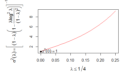
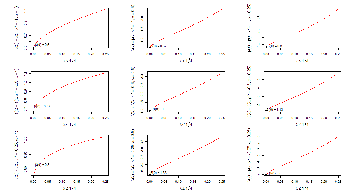
Remark 2. Robustness under Pa-type models has received quite some attention in the literature (see for instance Hubert et al., 2013, and the references therein) while the classical estimators such as Hill’s (1975) estimator are known to be highly non robust against outliers. The estimator $\hat{\alpha}_{r,k,n}$ provides a way to robustify the Hill estimator $H_{1,k,n}$ using a trimming procedure (with $r>1$). Trimming of course makes the estimator more robust against outliers, but decreases the efficiency of the estimator. This is illustrated in Figure 8 of Appendix 3, plotting the functions $\sigma^{2}(\lambda)$ and $\beta(\lambda)$ for $\lambda\in[0,1/4]$. The robustness properties of the estimation procedures presented here will be studied elsewhere.

References

• [1] I.B. Aban and M.M. Meerschaert (2004). Generalized least squares estimators for the thickness of heavy tails. Journal of Statistical Planning and Inference 119, 341–352.
• [2] I.B. Aban, M.M. Meerschaert, and A.K. Panorska (2006). Parameter Estimation for the Truncated Pareto Distribution, Journal of the American Statistical Association: Theory and Methods 101(473), 270–277.
• [3] Beirlant, J., Vynckier, P. and Teugels, J. (1996). Tail index estimation, Pareto quantile plots and regression diagnostics. J. Amer. Statist. Assoc., 91, 1659-1667.
• [4] Beirlant, J., Goegebeur, Y., Teugels, J. and Segers, J., 2004. Statistics of Extremes: Theory and Applications, Wiley, UK.
• [5] Clark, D.R. (2013). A note on the upper-truncated Pareto distribution. In Proc. of the Enterprise Risk Management Symposium, April 22-24, Chicago IL.
• [6] Dekkers, A., Einmahl, J. and de Haan, L. (1989). A moment estimator for the index of an extreme-value distribution. Ann. Statist., 17, 1795-1832.
• [7] de Haan, L. and Ferreira, A., 2006. Extreme Value Theory: an Introduction, Springer Science and Business Media, LLC, New York.
• [8] Hill, B.M. (1975). A simple general approach about the tail of a distribution. Annals of Statistics 3, 1163-1174.
• [9] Hubert, M., Dierckx, G. and Vanpaemel, D. (2013). Detecting influential data points for the Hill estimator in Pareto-type distributions. Computational and Statistical Data Analysis 65, 13-28.
• [10] Nuyts, J. (2010). Inference about the tail of a distribution: improvement on the Hill estimator. International Journal of Mathematics and Mathematical Sciences, Article ID 924013.
• [11] Seneta, E., 1976. Regularly Varying Functions. Lecture Notes in Math. 508, Springer-Verlag, Berlin.
• [12] Weissman, I. (1978). Estimation of parameters and large quantiles based on the kk largest observations. Journal of the American Statistical Association 73, 812-815.