跳到论文正文
W Papers独立论文阅读器 arXiv:1410.3468 论文正文 计算阅读时间 · 0%
引用这篇论文根据当前论文元数据生成,正式投稿前建议核对。


License: arXiv.org perpetual non-exclusive license
arXiv:1410.3468v3 [astro-ph.CO] 19 May 2015

An exploration of galaxy-galaxy lensing and galaxy clustering in the Millennium-XXL simulation

Laura Marian ††thanks: l.marian@sussex.ac.uk Affiliation:  Department of Physics and Astronomy, University of Sussex, Brighton BN1 9QH, UK Affiliation:  Argelander-Institute for Astronomy, Auf dem Hügel 71, D-53121 Bonn, Germany    Robert E. Smith & Raul E. Angulo Affiliation:  Department of Physics and Astronomy, University of Sussex, Brighton BN1 9QH, UK Affiliation:  Max-Planck Institute for Astrophysics, Karl-Schwarzschild-Str. 1, Garching, D-85748, Germany Affiliation:  Centro de Estudios de Fisica del Cosmos de Aragon, Plaza San Juan 1, Planta-2, 44001, Teruel, Spain
Abstract

The combination of galaxy-galaxy lensing and galaxy clustering data has the potential to simultaneously constrain both the cosmological and galaxy formation models. In this paper we perform a comprehensive exploration of these signals and their covariances through a combination of analytic and numerical approaches. First, we derive analytic expressions for the projected galaxy correlation function and stacked tangential shear profile and their respective covariances, which include Gaussian and discreteness noise terms. Secondly, we measure these quantities from mock galaxy catalogues obtained from the Millennium-XXL simulation and semi-analytic models of galaxy formation. We find that on large scales (R>10​h−1​MpcR>10\,h^{-1}{\rm Mpc}), the galaxy bias is roughly linear and deterministic. On smaller scales (R≲5​h−1​MpcR\lesssim 5\,h^{-1}{\rm Mpc}) the bias is a complicated function of scale and luminosity, determined by the different spatial distribution and abundance of satellite galaxies present when different magnitude cuts are applied, as well as by the mass dependence of the host haloes on magnitude. Our theoretical model for the covariances provides a reasonably good description of the measured ones on small and large scales. However, on intermediate scales (1<R<10​h−1​Mpc)(1<R<10\,h^{-1}{\rm Mpc}), the predicted errors are ∼\sim2–3 times smaller, suggesting that the inclusion of higher-order, non-Gaussian terms in the covariance will be required for further improvements. Importantly, both our theoretical and numerical methods show that the galaxy-galaxy lensing and clustering signals have a non-zero cross-covariance matrix with significant bin-to-bin correlations. Future surveys aiming to combine these probes must take this into account in order to obtain unbiased and realistic constraints.

Keywords: 
Cosmology: theory. Gravitational lensing: weak

1 Introduction

Since the first pioneering attempt to measure the galaxy-galaxy lensing (hereafter GGL) signal by Tyson et al. (1984), there have been significant technological developments in deep and wide-field astronomy, which have lead to the emergence of GGL as one of the most promising probes for simultaneously constraining both the cosmological and galaxy formation models.

The first robust detection of the GGL signal was made by Brainerd, Blandford & Smail (1996) using 90 arcmin2 of imaging data from the 5m Palomar telescope. They showed that whilst the tangential shear profile around individual galaxies was too weak to be measured, the stacked signal around all lens galaxies could be detected with high signal-to-noise. Since then there has been a rapid explosion in the field: the addition of the Wide-Field Camera to the Hubble Space Telescope enabled a number of key GGL studies (Griffiths et al., 1996; Hudson et al., 1998; dell’Antonio & Tyson, 1996; Leauthaud et al., 2012). The improvement of ground-based facilities such as the Canada-France-Hawaii Telescope has also led to significant developments (Wilson et al., 2001; Hoekstra, Yee & Gladders, 2004; Parker et al., 2007; van Uitert et al., 2011; Hudson et al., 2015; Velander et al., 2014). However, perhaps the most prolific work in this area comes from the analysis of the data from the Sloan Digital Sky Survey (hereafter SDSS) (McKay et al., 2001; Guzik & Seljak, 2001; Guzik & Seljak, 2002; Sheldon et al., 2004; Hirata et al., 2004; Mandelbaum et al., 2005; Mandelbaum et al., 2006c; Mandelbaum et al., 2006a; Mandelbaum et al., 2006b; Johnston et al., 2007; Sheldon et al., 2009b; Sheldon et al., 2009a; Nakajima et al., 2012; Mandelbaum et al., 2013). All these works have revealed that the GGL signal is a complex function depending on a number of galaxy properties, such as luminosity, colour, spectral type etc. The key importance of GGL is that it enables one to make a direct link from galaxy properties to the underlying dark matter distribution. Indeed, these works have also constrained the mass, density profiles, ellipticity of the dark matter haloes hosting the lens galaxies.

One of the first to realize that cosmic shear could help to simultaneously constrain galaxy formation and cosmology, through directly measuring the bias, was Schneider (1998). Schneider’s approach of using aperture mass filters was implemented by Hoekstra et al. (2002) who directly measured galaxy bias, establishing that it was a complicated function of scale. This approach was further theoretically developed for the Halo Occupation Distribution (hereafter HOD) framework by Guzik & Seljak (2001) and later Seljak et al. (2005) and Yoo et al. (2006). More recent work has been performed by Cacciato et al. (2009); Cacciato et al. (2013) who have combined the results from GGL and galaxy clustering (hereafter GC) studies, along with measurements of the galaxy luminosity function (hereafter GLF) from SDSS to constrain the parameters of the Conditional Luminosity Function (hereafter CLF) model – which fully specifies the link between a given dark matter halo and the galaxies it hosts, albeit with assumptions about the functional form of the CLF (Yang, Mo & van den Bosch, 2003; van den Bosch et al., 2013). An interesting result to emerge from this work, was that if one did not include the GGL measurements in the analysis, then equally good fits to the CLF model parameters could be obtained for either WMAP1 or WMAP3 cosmology (Spergel et al., 2003; Spergel et al., 2007). Including the GGL data broke this degeneracy and identified the WMAP3 parameters as the preferred cosmological model. See also the very recent works of Miyatake et al. (2013); More et al. (2014).

Whilst there has been significant progress in attempting to understand and interpret the GGL signal (Baldauf et al., 2010; Saghiha et al., 2012, see also), our understanding of how to perform a robust likelihood analysis with such data sets has been lacking. For example, in the recent development of the CLF framework (van den Bosch et al., 2013; Cacciato et al., 2013; More et al., 2013), the GGL and GLF measurements were taken to have diagonal covariance matrices, and the GC covariance matrix was obtained from jackknife estimation. Moreover, these probes were assumed to have zero cross-covariance. This is clearly a simplification that future large data sets analyses should improve on. A better analysis of the errors was performed by Leauthaud et al. (2012) who used numerical simulations to estimate the covariance matrices of the GGL and GC measurements, while Mandelbaum et al. (2013) used the jackknife approach. The very recent works of Miyatake et al. (2013); More et al. (2014) also had an improved error analysis. However, again in their analyses the cross-covariance of the two measurements was assumed to be negligible.

If upcoming surveys such as the Dark Energy Survey (DES), the Javalambre-Physics of the Accelerated Universe Astrophysical Survey (J-PAS), Euclid, and the Large Synoptic Survey Telescope (LSST) are to optimally constrain the cosmological model, then it is inevitable that they must also jointly constrain the model of galaxy formation. The best way to do this will be to combine the GGL, GC and GLF measurements. This will require not only accurate models for the signals themselves, but also accurate modelling of the covariance and cross-covariance matrices of these probes.

In this paper we develop an analytical framework to compute both the covariance and cross-covariance of GC and GGL. Our work builds upon the analysis of the earlier work of Jeong, Komatsu & Jain (2009) for GGL and that of Smith & Marian (2014); Smith & Marian (2015) for the GC signal. We then use the semi-analytic galaxy catalogues and dark matter distribution from the Millennium-XXL (hereafter MXXL) simulation (Angulo et al., 2012) to directly measure these observables and their associated auto- and cross-covariances, for several bins in luminosity. Unlike the CLF approach, semi-analytic models (hereafter SAM) make no direct assumption on how galaxies populate dark matter haloes. Instead, they attempt to model the relevant physical processes for galaxy formation and evolution, and how these are affected by environment and assembly history. Thus, the nonlinearity and stochasticity of galaxy bias are predictions, not assumptions in our study.

The paper is structured as follows. In §2 we present the necessary theoretical expressions for modelling the stacked tangential shear profiles and projected galaxy clustering signals. In §3 we present expressions for their associated auto- and cross-covariances. In §4 we provide an overview of the MXXL-simulation and the SAM galaxy catalogues that we use. In §5 we present the measurements of the GGL and GC signals for a set of luminosity bins, and compare them with the predictions from the theory. In §6 we present our results for the GC and GGL covariance and cross-covariance matrices. In §7 we summarize our findings and draw our conclusions.

2 Theoretical predictions for the GGL and GC signals

In this section we present theoretical expressions for the stacked tangential shear signal of a population of galaxy lenses and the signal for the projected galaxy correlation function.

2.1 Overview of required lensing ingredients

In the flat-sky approximation, the complex shear is written in terms of the convergence as (Bartelmann & Schneider, 2001)

γ⁡(𝜽)=1π​∫𝐑2d2​θ′​κ​(𝜽′)​𝒟​(𝜽−𝜽′),\gamma({\mbox{\boldmath$\theta$}})=\frac{1}{\pi}\int_{\mathbf{R}^{2}}d^{2}\theta^{\prime}\kappa({\mbox{\boldmath$\theta$}}^{\prime})\mathcal{D}({\mbox{\boldmath$\theta$}}-{\mbox{\boldmath$\theta$}}^{\prime})\ , (1)

where the lensing kernel is defined to be,

𝒟⁡(𝜽)≡(θy2−θx2−2​i​θx​θy)/|𝜽|4,\mathcal{D}({\mbox{\boldmath$\theta$}})\equiv(\theta_{y}^{2}-\theta_{x}^{2}-2i\theta_{x}\theta_{y})/|{\mbox{\boldmath$\theta$}}|^{4}, (2)

with θx\theta_{x} and θy\theta_{y} being the Cartesian components of the Euclidean vector 𝜽=(θx,θy){\mbox{\boldmath$\theta$}}=(\theta_{x},\theta_{y}). These equations can be written in Fourier space as:

γ⁡(𝒍)=1π​κ​(𝒍)​𝒟​(𝒍),with​𝒟​(𝒍)=π​lx2−ly2+2​i​lx​ly|𝒍|2,\gamma({\mbox{\boldmath$l$}})=\frac{1}{\pi}\kappa({\mbox{\boldmath$l$}})\mathcal{D}({\mbox{\boldmath$l$}}),\hskip 5.69046pt{\rm with}\hskip 5.69046pt\mathcal{D}({\mbox{\boldmath$l$}})=\pi\frac{l_{x}^{2}-l_{y}^{2}+2il_{x}l_{y}}{|{\mbox{\boldmath$l$}}|^{2}}, (3)

where lxl_{x} and lyl_{y} are the Cartesian components of the vector 𝒍l; γ⁡(𝒍)\gamma({\mbox{\boldmath$l$}}) and 𝒟⁡(𝒍)\mathcal{D}({\mbox{\boldmath$l$}}) and are the Fourier transforms of γ⁡(𝜽)\gamma({\mbox{\boldmath$\theta$}}) and 𝒟⁡(𝜽)\mathcal{D}({\mbox{\boldmath$\theta$}}) respectively. From Eq. (3), the complex shear can also be written using the polar coordinates of the Fourier vector 𝒍l as:

γ⁡(𝒍)=γ1​(𝒍)+i​γ2​(𝒍)=κ⁡(𝒍)​[cos⁡(2​ϕ𝒍)+i​sin⁡(2​ϕ𝒍)].\gamma({\mbox{\boldmath$l$}})=\gamma_{1}({\mbox{\boldmath$l$}})+i\gamma_{2}({\mbox{\boldmath$l$}})=\kappa({\mbox{\boldmath$l$}})[\cos(2\phi_{{\mbox{\boldmath$l$}}})+i\sin(2\phi_{{\mbox{\boldmath$l$}}})]. (4)

The tangential shear at position 𝜽\theta with respect to position 𝜽0{\mbox{\boldmath$\theta$}}_{0} (where 𝜽\theta and 𝜽0{\mbox{\boldmath$\theta$}}_{0} are defined with respect to the same origin), is:

γt​(𝜽,𝜽0)=−γ1​(𝜽)​cos⁡(2​ϕ𝜽−𝜽0)−γ2​(𝜽)​sin⁡(2​ϕ𝜽−𝜽0),\gamma_{t}({\mbox{\boldmath$\theta$}};{\mbox{\boldmath$\theta$}}_{0})=-\gamma_{1}({\mbox{\boldmath$\theta$}})\cos(2\phi_{{\mbox{\boldmath$\theta$}}-{\mbox{\boldmath$\theta$}}_{0}})-\gamma_{2}({\mbox{\boldmath$\theta$}})\sin(2\phi_{{\mbox{\boldmath$\theta$}}-{\mbox{\boldmath$\theta$}}_{0}}), (5)

where ϕ𝜽−𝜽0\phi_{{\mbox{\boldmath$\theta$}}-{\mbox{\boldmath$\theta$}}_{0}} is the polar angle of the relative position vector 𝜽−𝜽0{\mbox{\boldmath$\theta$}}-{\mbox{\boldmath$\theta$}}_{0}. Combining the last two equations, one can write:

γt(𝜽;𝜽0)=−∫d2​l(2​π)2κ(𝒍)cos[2(ϕ𝜽−𝜽0−ϕ𝒍)]ei​𝒍⋅𝜽.\gamma_{t}({\mbox{\boldmath$\theta$}};{\mbox{\boldmath$\theta$}}_{0})=-\int\frac{d^{2}l}{(2\pi)^{2}}\kappa({\mbox{\boldmath$l$}})\cos[2(\phi_{{\mbox{\boldmath$\theta$}}-{\mbox{\boldmath$\theta$}}_{0}}-\phi_{{\mbox{\boldmath$l$}}})]\,e^{i\,{\mbox{\boldmath$l$}}\cdot{\mbox{\boldmath$\theta$}}}\ . (6)

Finally, we define the azimuthal average of the tangential shear as:

γt,a​(θ,𝜽0)=∫02​πd​ϕ𝜽−𝜽02​π​γt​(𝜽,𝜽0).\gamma_{t,a}(\theta;{\mbox{\boldmath$\theta$}}_{0})=\int_{0}^{2\pi}\frac{d\phi_{{\mbox{\boldmath$\theta$}}-{\mbox{\boldmath$\theta$}}_{0}}}{2\pi}\gamma_{t}({\mbox{\boldmath$\theta$}};{\mbox{\boldmath$\theta$}}_{0}). (7)

With the help of the very useful Bessel relation

Jn​(x)=∫α2​π−αd​ϕ2​π​ei⁡[n​ϕ−x​sin⁡(ϕ)],J_{n}(x)=\int_{\alpha}^{2\pi-\alpha}\frac{d\phi}{2\pi}\,e^{i\,[n\phi-x\sin(\phi)]}\ , (8)

one obtains the following equation which will recur many times in this section:

J2(x)=−∫02​πd​ϕ2​πcos[2(ϕ−ϕ′)]ei​x​cos⁡(ϕ−ϕ′).J_{2}(x)=-\int_{0}^{2\pi}\frac{d\phi}{2\pi}\cos[2(\phi-\phi^{\prime})]e^{i\,x\cos(\phi-\phi^{\prime})}. (9)

Therefore the azimuthal average of the tangential shear is:

γt,a​(θ,𝜽0)=∫d2​l(2​π)2​κ​(𝒍)​J2​(l​θ)​ei​𝒍⋅𝜽0.{\gamma_{t,a}}(\theta;{\mbox{\boldmath$\theta$}}_{0})=\int\frac{d^{2}l}{(2\pi)^{2}}\kappa({\mbox{\boldmath$l$}})J_{2}(l\theta)e^{i\,{\mbox{\boldmath$l$}}\cdot{\mbox{\boldmath$\theta$}}_{0}}. (10)

2.2 Estimator for the stacked tangential shear

In galaxy-galaxy lensing, the signal of individual lenses is very weak, so in order to improve the signal-to-noise of this probe, one has to stack several lenses. Suppose there is a population of NgN_{g} galaxy lenses at positions 𝒙i{\mbox{\boldmath$x$}}_{i} in a chosen coordinate system. Suppose also the total area of the survey to be ∫d2​x=Ωs\int d^{2}x=\Omega_{s}. The number density of these lenses can be written as a sum over their positions:

ng​(𝒙)=∑i=1NgδD​(𝒙−𝒙i),n_{g}({\mbox{\boldmath$x$}})=\sum_{i=1}^{N_{g}}\delta_{D}({\mbox{\boldmath$x$}}-{\mbox{\boldmath$x$}}_{i})\ , (11)

where 𝒙x is a 2D vector in the survey area. Using the above equation, an estimator for the tangential shear of such a lens population at an arbitrary position 𝜽\theta with respect to the location of the galaxy centres 𝒙i{\mbox{\boldmath$x$}}_{i} is (Jeong, Komatsu & Jain, 2009):

γ^tg​(𝜽)\displaystyle\widehat{\gamma}_{t}^{g}({\mbox{\boldmath$\theta$}}) =\displaystyle= 1Ng​∑i=1Ngγt​(𝒙i+𝜽,𝒙i)\displaystyle\frac{1}{N_{g}}\sum_{i=1}^{N_{g}}\gamma_{t}({\mbox{\boldmath$x$}}_{i}+{\mbox{\boldmath$\theta$}};{\mbox{\boldmath$x$}}_{i}){} (12)
=\displaystyle= 1Ng​∫Ωsd2​x​ng​(𝒙)​γt​(𝒙+𝜽,𝒙).\displaystyle\frac{1}{N_{g}}\int_{\Omega_{s}}d^{2}x\,n_{g}({\mbox{\boldmath$x$}})\gamma_{t}({\mbox{\boldmath$x$}}+{\mbox{\boldmath$\theta$}};{\mbox{\boldmath$x$}})\ .

We define the fluctuation in the number density of lenses as ng​(𝒙)=n¯g​[1+δg​(𝒙)]n_{g}({\mbox{\boldmath$x$}})=\bar{n}_{g}[1+\delta_{g}({\mbox{\boldmath$x$}})], where the mean angular density of lens galaxies is n¯g=Ng/Ωs\bar{n}_{g}=N_{g}/\Omega_{s}. At this point we also introduce the definitions of the convergence and galaxy density auto- and cross-power spectra, which shall be used throughout this paper:

⟨κ⁡(𝒍)​κ​(𝒍′)⟩\displaystyle\langle\kappa({\mbox{\boldmath$l$}})\kappa({\mbox{\boldmath$l$}}^{\prime})\rangle =\displaystyle= (2​π)2​δD​(𝒍+𝒍′)​𝒞κ​κ​(l);\displaystyle(2\pi)^{2}\delta_{D}({\mbox{\boldmath$l$}}+{\mbox{\boldmath$l$}}^{\prime})\mathcal{C}_{\kappa\kappa}(l)\ ;
⟨δg​(𝒍)​δg​(𝒍′)⟩\displaystyle\langle\delta_{g}({\mbox{\boldmath$l$}})\delta_{g}({\mbox{\boldmath$l$}}^{\prime})\rangle =\displaystyle= (2​π)2​δD​(𝒍+𝒍′)​𝒞g​g​(l);\displaystyle(2\pi)^{2}\delta_{D}({\mbox{\boldmath$l$}}+{\mbox{\boldmath$l$}}^{\prime})\mathcal{C}_{gg}(l)\ ;
⟨δg​(𝒍)​κ​(𝒍′)⟩\displaystyle\langle\delta_{g}({\mbox{\boldmath$l$}})\kappa({\mbox{\boldmath$l$}}^{\prime})\rangle =\displaystyle= (2​π)2​δD​(𝒍+𝒍′)​𝒞g​κ​(l).\displaystyle(2\pi)^{2}\delta_{D}({\mbox{\boldmath$l$}}+{\mbox{\boldmath$l$}}^{\prime})\mathcal{C}_{g\kappa}(l)\ . (13)

Since the tangential shear with respect to an origin 𝟎{\bf 0} vanishes on average ⟨γt​(𝜽|𝟎)⟩=0\langle\gamma_{t}({\mbox{\boldmath$\theta$}}|{\bf 0})\rangle=0, the ensemble average of the estimator in Eq. (12) is

⟨γ^tg​(𝜽)⟩\displaystyle\langle\widehat{\gamma}_{t}^{g}({\mbox{\boldmath$\theta$}})\rangle =\displaystyle= 1Ng​∫Ωsd2​x​⟨ng​(𝒙)​γt​(𝒙+𝜽,𝒙)⟩\displaystyle\frac{1}{N_{g}}\int_{\Omega_{s}}d^{2}x\,\langle n_{g}({\mbox{\boldmath$x$}})\gamma_{t}({\mbox{\boldmath$x$}}+{\mbox{\boldmath$\theta$}};{\mbox{\boldmath$x$}})\rangle{} (14)
=\displaystyle= 1Ωs​∫Ωsd2​x​⟨δg​(𝒙)​γt​(𝒙+𝜽,𝒙)⟩\displaystyle\frac{1}{\Omega_{s}}\int_{\Omega_{s}}d^{2}x\,\langle\delta_{g}({\mbox{\boldmath$x$}})\gamma_{t}({\mbox{\boldmath$x$}}+{\mbox{\boldmath$\theta$}};{\mbox{\boldmath$x$}})\rangle{}
=\displaystyle= ⟨δg​(𝟎)​γt​(𝜽,𝟎)⟩\displaystyle\langle\delta_{g}({\bf 0})\gamma_{t}({\mbox{\boldmath$\theta$}};{\bf 0})\rangle{}
=\displaystyle= −∫d2​l(2​π)2𝒞g​κ(l)cos[2(ϕ𝜽−ϕ𝒍)]ei​𝒍⋅𝜽.\displaystyle-\int\frac{d^{2}l}{(2\pi)^{2}}\mathcal{C}_{g\kappa}(l)\cos[2(\phi_{{\mbox{\boldmath$\theta$}}}-\phi_{{\mbox{\boldmath$l$}}})]e^{i\,{\mbox{\boldmath$l$}}\cdot{\mbox{\boldmath$\theta$}}}.

In the above we have also used the homogeneity of the Universe, which makes the ensemble average of two cosmological fields to be invariant under translations. We shall take advantage extensively of this property throughout this work. With Eq. (9), we arrive at the azimuthally-averaged expression for the ensemble average of the stacked shear estimator:

⟨γ^t,ag​(θ)⟩=∫d2​l(2​π)2​𝒞g​κ​(l)​J2​(l​θ).\langle\widehat{\gamma}_{t,a}^{g}(\theta)\rangle=\int\frac{d^{2}l}{(2\pi)^{2}}\mathcal{C}_{g\kappa}(l)J_{2}(l\theta). (15)

Our goal is to compare theory predictions with estimates from simulations, so we must take into account that the measured tangential shear is bin averaged and not just azimuthally averaged. We introduce the bin area:

A⁡(θi)≡∫02​πd​ϕ𝜽​∫θminiθmaxid​θ​θ=π⁡(θmaxi​ 2−θmini​ 2),A(\theta_{i})\equiv\int_{0}^{2\pi}d\phi_{\mbox{\boldmath$\theta$}}\int_{\theta_{\rm min}^{i}}^{\theta^{i}_{\rm max}}d\theta\,\theta=\pi\left(\theta^{i\,2}_{\rm max}-\theta^{i\,2}_{\rm min}\right), (16)

with θmini\theta^{i}_{\rm min} and θmaxi\theta^{i}_{\rm max} being the lower and upper bounds of the radial bin ii. The bin-averaged stacked tangential shear estimator is defined by

⟨γ¯^tg​(θi)⟩≡∫A⁡(θi)d2​θA⁡(θi)​⟨γ^tg​(𝜽)⟩=2​πA⁡(θi)​∫θminiθmaxid​θ​θ​⟨γ^t,ag​(θ)⟩\langle\widehat{\widebar{\gamma}}_{t}^{g}(\theta_{i})\rangle\equiv\int_{A(\theta_{i})}\frac{d^{2}\theta}{A(\theta_{i})}\langle\widehat{\gamma}_{t}^{g}({\mbox{\boldmath$\theta$}})\rangle=\frac{2\pi}{A(\theta_{i})}\int_{\theta^{i}_{\rm min}}^{\theta^{i}_{\rm max}}d\theta\,\theta\langle\widehat{\gamma}^{g}_{t,a}(\theta)\rangle (17)

Defining the bin-averaged Bessel function of order nn to be:

J¯n​(l​θi)≡∫A⁡(θi)d2​θA⁡(θi)​Jn​(l​θ),\widebar{J}_{n}(l\theta_{i})\equiv\int_{A(\theta_{i})}\frac{d^{2}\theta}{A(\theta_{i})}J_{n}(l\theta), (18)

and using Eq. (15), we write the final expression for the bin-averaged stacked tangential shear estimator

⟨γ¯^tg​(θi)⟩=∫d2​l(2​π)2​𝒞g​κ​(l)​J¯2​(l​θi).\langle\widehat{\widebar{\gamma}}_{t}^{g}(\theta_{i})\rangle=\int\frac{d^{2}l}{(2\pi)^{2}}\mathcal{C}_{g\kappa}(l)\widebar{J}_{2}(l\theta_{i}). (19)

2.3 The projected galaxy correlation function

We define the estimator for the projected galaxy correlation function to be:

w^gg​(R)≡∫02​πd​ϕ𝐑2​π​∫−χmaxχmaxd​χ​ξ^gg​(𝐫),\widehat{w}_{\rm gg}(R)\equiv\int_{0}^{2\pi}\frac{d\phi_{\bf R}}{2\pi}\int_{-\chi_{\rm max}}^{\chi_{\rm max}}d\chi\,\widehat{\xi}_{\rm gg}({\bf r}), (20)

where ξ^gg\widehat{\xi}_{\rm gg} is an estimator for the 3D galaxy correlation function, χmax\chi_{\rm max} is the comoving projection length, and the position vector 𝐫{\bf r} has the components {R,ϕ𝐑,χ}\{R,\phi_{\bf R},\chi\} in cylindrical coordinates. The estimator for the galaxy correlation function is discussed in section §A.2 of the appendix, here we just mention that it is unbiased, i.e. ⟨ξ^gg​(𝐫)⟩=ξgg​(𝐫)\langle\widehat{\xi}_{\rm gg}({\bf r})\rangle=\xi_{\rm gg}({\bf r}). Note that in this study we shall ignore redshift-space distortions, as for our chosen projection length χmax=100​h−1​Mpc\chi_{\rm max}=100\,\,h^{-1}{\rm Mpc}, their contribution to w^gg\widehat{w}_{\rm gg} is of ∼10%\sim 10\% on the largest scales that we consider and less otherwise (Baldauf et al., 2010). The galaxy correlation function can be written in terms of its Fourier transform, the galaxy power spectrum:

ξgg​(𝐫)\displaystyle\xi_{\rm gg}({\bf r}) =\displaystyle= ∫d3​k(2​π)3​𝒫gg​(k)​ei​𝒌⋅𝐫\displaystyle\int\frac{d^{3}k}{(2\pi)^{3}}\mathcal{P}_{\rm gg}(k)\,e^{i\,{\mbox{\boldmath$k$}}\cdot{\bf r}}{} (21)
=\displaystyle= ∫0∞d​k⟂(2​π)3​k⟂​∫∞∞d​kz​𝒫gg​(k)\displaystyle\int_{0}^{\infty}\frac{dk_{\perp}}{(2\pi)^{3}}k_{\perp}\int_{\infty}^{\infty}dk_{z}\mathcal{P}_{\rm gg}(k){}
×ei​kz​χ​∫02​πd​ϕ𝒌​ei​k⟂​R​cos⁡(ϕ𝐑−ϕ𝒌),\displaystyle\times\,e^{i\,k_{z}\chi}\int_{0}^{2\pi}d\phi_{\mbox{\boldmath$k$}}\,e^{i\,k_{\perp}R\cos(\phi_{\bf R}-\phi_{\mbox{\boldmath$k$}})},

where the second line follows from expressing the wavevector 𝒌k in cylindrical coordinates, with components {k⟂,ϕ𝒌,kz}\{k_{\perp},\phi_{\mbox{\boldmath$k$}},k_{z}\}. kzk_{z} is the component along the line-of-sight and the magnitude kk is defined in the standard way k=k⟂2+kz2k=\sqrt{k_{\perp}^{2}+k_{z}^{2}}. The expectation of the projected galaxy correlation function estimator may therefore be written

⟨w^gg​(R)⟩\displaystyle\langle\widehat{w}_{\rm gg}(R)\rangle\hskip-8.5359pt =\displaystyle= ∫0∞d​k⟂(2​π)2​k⟂​J0​(k⟂​R)​∫−∞∞d​kz​𝒫gg​(k)​∫−χmaxχmaxd​χ​ei​kz​χ\displaystyle\hskip-11.38092pt\int_{0}^{\infty}\hskip-5.69046pt\frac{dk_{\perp}}{(2\pi)^{2}}k_{\perp}J_{0}(k_{\perp}R)\hskip-2.84544pt\int_{-\infty}^{\infty}\hskip-11.38092ptdk_{z}\mathcal{P}_{\rm gg}(k)\int_{-\chi_{\rm max}}^{\chi_{\rm max}}\hskip-8.5359ptd\chi\,e^{i\,k_{z}\chi} (22)
=\displaystyle= 4​χmax​∫0∞d​k⟂(2​π)2​k⟂​J0​(k⟂​R)​∫0∞d​kz​𝒫gg​(k)​j0​(kz​χmax),\displaystyle\hskip-8.5359pt4\chi_{\rm max}\hskip-2.84544pt\int_{0}^{\infty}\hskip-5.69046pt\frac{dk_{\perp}}{(2\pi)^{2}}k_{\perp}J_{0}(k_{\perp}R)\int_{0}^{\infty}\hskip-8.5359ptdk_{z}\mathcal{P}_{\rm gg}(k)j_{0}(k_{z}\chi_{\rm max}),{}

where j0j_{0} is the zeroth order spherical Bessel function. Note that we can also obtain an expression for the ensemble average of our projected correlation function estimator in spherical coordinates, choosing a particular frame where 𝐫|𝐞𝐳{\bf r}\parallel{\bf e_{z}}

⟨w^gg​(R)⟩\displaystyle\langle\widehat{w}_{\rm gg}(R)\rangle\hskip-8.5359pt =\displaystyle= 2​∫0∞d​k(2​π)2​k2​𝒫gg​(k)​∫−χmaxχmaxd​χ​j0​(k​r)\displaystyle\hskip-8.5359pt2\int_{0}^{\infty}\hskip-5.69046pt\frac{dk}{(2\pi)^{2}}k^{2}\mathcal{P}_{\rm gg}(k)\int_{-\chi_{\rm max}}^{\chi_{\rm max}}\hskip-11.38092ptd\chi\,j_{0}(kr){} (24)
=\displaystyle= 4​∫0∞d​k(2​π)2​k2​𝒫gg​(k)​∫0χmaxd​χ​j0​(k​R2+χ2),\displaystyle\hskip-8.5359pt4\int_{0}^{\infty}\hskip-5.69046pt\frac{dk}{(2\pi)^{2}}k^{2}\mathcal{P}_{\rm gg}(k)\int_{0}^{\chi_{\rm max}}\hskip-11.38092ptd\chi\,j_{0}(k\sqrt{R^{2}+\chi^{2}}),

where in the last equality we took advantage of the fact that the result did not depend on our particular choice of frame, and switched back to cylindrical coordinates. Whilst Eqs. () and (24) are expected to yield the same result, the evaluation of the latter should more accurate since it involves a single Bessel function integral.

Finally, we may apply the Limber approximation to simplify Eq. (). In this approximation it is only modes that are transverse to the line-of-sight which contribute to the power spectrum integral, and so the second integral in Eq. (22)) becomes,

∫−∞∞d​kz​𝒫gg​(k⟂2+kz2)​∫−χmaxχmaxd​χ​ei​kz​χ\displaystyle\int_{-\infty}^{\infty}dk_{z}\mathcal{P}_{\rm gg}(\sqrt{k_{\perp}^{2}+k_{z}^{2}})\int_{-\chi_{\rm max}}^{\chi_{\rm max}}d\chi\,e^{i\,k_{z}\chi}{} (25)
≈𝒫gg​(k⟂)​∫−χmaxχmaxd​χ​∫−∞∞d​kz​ei​kz​χ=2​π​𝒫gg​(k⟂).\displaystyle\hskip-170.71652pt\approx\mathcal{P}_{\rm gg}(k_{\perp})\int_{-\chi_{\rm max}}^{\chi_{\rm max}}d\chi\int_{-\infty}^{\infty}dk_{z}\,e^{i\,k_{z}\chi}=2\pi\mathcal{P}_{\rm gg}(k_{\perp}).

Using this relation in Eq. (22) we find that the Limber-approximated ensemble average of the projected galaxy correlation function estimator is therefore11 1 Note that this result can also be obtained if in Eq. () one takes χmax→∞\chi_{\rm max}\rightarrow\infty.:

⟨w^ggL​(R)⟩=∫0∞d​k⟂2​π​k⟂​𝒫gg​(k⟂)​J0​(k⟂​R).\langle\widehat{w}_{\rm gg}^{L}(R)\rangle=\int_{0}^{\infty}\frac{dk_{\perp}}{2\pi}k_{\perp}\mathcal{P}_{\rm gg}(k_{\perp})J_{0}(k_{\perp}R). (26)

3 Signal covariance matrices

In this section we compute the auto- and cross-covariance matrices of the stacked tangential shear signal and the projected galaxy correlation function.

3.1 The covariance matrix of the stacked tangential shear estimator

The definition of the covariance of the estimator in Eq. (12) is

Cov⁡[γ^tg]​(𝜽1,𝜽2)=⟨γ^tg​(𝜽1)​γ^tg​(𝜽2)⟩−⟨γ^tg​(𝜽1)⟩​⟨γ^tg​(𝜽2)⟩{\rm Cov}[\widehat{\gamma}_{t}^{g}]({\mbox{\boldmath$\theta$}}_{1},{\mbox{\boldmath$\theta$}}_{2})=\langle\widehat{\gamma}_{t}^{g}({\mbox{\boldmath$\theta$}}_{1})\widehat{\gamma}_{t}^{g}({\mbox{\boldmath$\theta$}}_{2})\rangle-\langle\widehat{\gamma}_{t}^{g}({\mbox{\boldmath$\theta$}}_{1})\rangle\langle\widehat{\gamma}_{t}^{g}({\mbox{\boldmath$\theta$}}_{2})\rangle (27)

The bin-averaged estimate of the GGL covariance is defined according to Eq. (17) as:

Cov⁡[γ¯^tg]​(θi,θj)≡∫Ai∫Ajd2​θ1Ai​d2​θ2Aj​Cov​[γ^tg]​(𝜽1,𝜽2).{\rm Cov}[\widehat{\widebar{\gamma}}_{t}^{g}](\theta_{i},\theta_{j})\equiv\int_{A_{i}}\int_{A_{j}}\frac{d^{2}\theta_{1}}{A_{i}}\frac{d^{2}\theta_{2}}{A_{j}}{\rm Cov}[\widehat{\gamma}_{t}^{g}]({\mbox{\boldmath$\theta$}}_{1},{\mbox{\boldmath$\theta$}}_{2}). (28)

In appendix A.1 we provide the complete details of the derivation of the covariance of the stacked tangential shear profiles. The main result is (c.f. Eq. (73)):

Cov⁡[γ¯^tg]​(θi,θj)\displaystyle{\rm Cov}[\widehat{\widebar{\gamma}}_{t}^{g}](\theta_{i},\theta_{j}) =\displaystyle= 1Ωs∫0∞d2​l(2​π)2J¯2(lθi)J¯2(lθj)×\displaystyle\frac{1}{\Omega_{s}}\int_{0}^{\infty}\frac{d^{2}l}{(2\pi)^{2}}\,\widebar{J}_{2}(l\theta_{i})\widebar{J}_{2}(l\theta_{j})\times{} (29)
{𝒞g​κ2​(l)+[𝒞κ​κ​(l)+σγ22​n¯s]​[𝒞gg​(l)+1n¯g]},\displaystyle\hskip-45.52458pt\left\{\mathcal{C}_{g\kappa}^{2}(l)+\left[\mathcal{C}_{\kappa\kappa}(l)+\frac{\sigma_{\gamma}^{2}}{2\bar{n}_{s}}\right]\left[\mathcal{C}_{\rm gg}(l)+\frac{1}{\bar{n}_{g}}\right]\right\},

where σγ2/2=σγ12=σγ22\sigma_{\gamma}^{2}/2=\sigma_{\gamma_{1}}^{2}=\sigma_{\gamma_{2}}^{2} is the variance per shear component in the measurement of one source galaxy, and n¯s\bar{n}_{s} is the mean angular density of the source galaxies.

3.2 The covariance matrix of the projected galaxy correlation function estimator

The azimuthally-averaged covariance of the projected correlation function estimator can be written as a projection of the covariance of the estimator for the 3D galaxy correlation function, which we denote ξ^gg\widehat{\xi}_{\rm gg}. Hence,

Cov⁡[w^gg]​(R1,R2)\displaystyle{\rm Cov}[\widehat{w}_{\rm gg}](R_{1},R_{2})\hskip-8.5359pt =\displaystyle= ∫02​πd​ϕ𝐑12​π​d​ϕ𝐑22​π​∫−χmaxχmaxd​χ1​d​χ2​Cov​[ξ^gg]​(𝐫1,𝐫2).\displaystyle\hskip-11.38092pt\int_{0}^{2\pi}\hskip-2.84544pt\frac{d\phi_{{\bf R}_{1}}}{2\pi}\hskip-2.84544pt\frac{d\phi_{{\bf R}_{2}}}{2\pi}\int_{-\chi_{\rm max}}^{\chi_{\rm max}}\hskip-19.91684ptd\chi_{1}d\chi_{2}\,{\rm Cov}[\widehat{\xi}_{\rm gg}]({\bf r}_{1},{\bf r}_{2}).{}

In the appendix A.2 we provide complete details of the derivation of the covariance matrix of ξ^gg\widehat{\xi}_{\rm gg} and the final result is given by Eq. (84). On combining the equation above and Eq. (84), we arrive at the expression for the azimuthally-averaged covariance of the projected galaxy correlation function estimator:

Cov⁡[w^gg]​(R1,R2)\displaystyle{\rm Cov}[\widehat{w}_{\rm gg}](R_{1},R_{2}) =1Vs{8χmax2∫0∞d​k⟂(2​π)2k⟂J0(k⟂R1)J0(k⟂R2)\displaystyle\hskip-19.91684pt=\frac{1}{V_{s}}\left\{8\chi^{2}_{\rm max}\int_{0}^{\infty}\hskip-5.69046pt\frac{dk_{\perp}}{(2\pi)^{2}}k_{\perp}J_{0}(k_{\perp}R_{1})J_{0}(k_{\perp}R_{2})\right.{} (30)
×∫−∞∞d​kz​j02​(kz​χmax)​𝒫gg​(k⟂2+kz2)​[𝒫gg​(k⟂2+kz2)+2​(1+α)n¯g]\displaystyle\hskip-99.58464pt\left.\times\int_{-\infty}^{\infty}\hskip-5.69046ptdk_{z}j_{0}^{2}(k_{z}\chi_{\rm max})\mathcal{P}_{\rm gg}(\sqrt{k_{\perp}^{2}+k_{z}^{2}})\left[\mathcal{P}_{\rm gg}(\sqrt{k_{\perp}^{2}+k_{z}^{2}})+\frac{2(1+\alpha)}{\bar{n}_{g}}\right]\right.{}
+2n¯g2[wgg(R1)+2χmax(1+α)2]δD​(R1−R2)2​π​R1},\displaystyle\hskip-93.89418pt\left.\,+\,\frac{2}{\bar{n}_{g}^{2}}\left[w_{\rm gg}(R_{1})+2\chi_{\rm max}(1+\alpha)^{2}\right]\frac{\delta_{D}(R_{1}-R_{2})}{2\pi R_{1}}\right\}\,,\hskip-113.81102pt

where α\alpha is a constant quantifying how dense the random catalogue used to estimate the correlation function is relative to the galaxy data (see §A.2 for more details). Note that in the above n¯g\bar{n}_{g} is the mean galaxy volume density, whereas in §3.1 the same notation is used for the mean angular density of lens galaxies. As in the case of the ensemble-averaged projected galaxy correlation function estimator, here too we apply the Limber approximation to simplify the above result. The Limber-approximated covariance is given by:

CovL​[w^gg]​(R1,R2)\displaystyle{\rm Cov^{L}}[\widehat{w}_{\rm gg}](R_{1},R_{2}) =1Vs{4χmax∫0∞d​k⟂2​πk⟂J0(k⟂R1)J0(k⟂R2)\displaystyle\hskip-19.91684pt=\frac{1}{V_{s}}\left\{4\chi_{\rm max}\int_{0}^{\infty}\hskip-2.84544pt\frac{dk_{\perp}}{2\pi}\,k_{\perp}J_{0}(k_{\perp}R_{1})J_{0}(k_{\perp}R_{2})\right.{} (31)
×𝒫gg​(k⟂)​[𝒫gg​(k⟂)+2​(1+α)n¯g]\displaystyle\left.\hskip-85.35826pt\,\times\,\mathcal{P}_{\rm gg}(k_{\perp})\left[\mathcal{P}_{\rm gg}(k_{\perp})+\frac{2(1+\alpha)}{\bar{n}_{g}}\right]\right.{}
+2n¯g2[wggL(R1)+2χmax(1+α)2]δD​(R1−R2)2​π​R1}.\displaystyle\left.\hskip-85.35826pt\,+\,\frac{2}{\bar{n}_{g}^{2}}\left[w_{\rm gg}^{L}(R_{1})+2\chi_{\rm max}(1+\alpha)^{2}\right]\frac{\delta_{D}(R_{1}-R_{2})}{2\pi R_{1}}\right\}.

Note that the survey volume can be expressed as Vs=2​χmax​AsV_{s}=2\chi_{\rm max}A_{s}, where AsA_{s} denotes the transverse area of the survey. If χmax→∞\chi_{\rm max}\rightarrow\infty, then we also have Vs→∞V_{s}\rightarrow\infty and the Limber-approximated covariance becomes:

limχmax→∞CovL​[w^gg]​(R1,R2)\displaystyle\hskip-8.5359pt\lim_{\chi_{\rm max}\rightarrow\infty}\hskip-8.5359pt{\rm Cov^{L}}[\widehat{w}_{\rm gg}](R_{1},R_{2}) =2As{∫0∞d​k⟂2​πk⟂J0(k⟂R1)J0(k⟂R2)\displaystyle\hskip-17.07182pt=\frac{2}{A_{s}}\left\{\int_{0}^{\infty}\hskip-2.84544pt\frac{dk_{\perp}}{2\pi}\,k_{\perp}J_{0}(k_{\perp}R_{1})J_{0}(k_{\perp}R_{2})\right.{}
×𝒫gg(k⟂)[𝒫gg(k⟂)+2​(1+α)n¯g]+(1+α)2n¯g2δD​(R1−R2)2​π​R1}.\displaystyle\left.\hskip-113.81102pt\,\times\,\mathcal{P}_{\rm gg}(k_{\perp})\left[\mathcal{P}_{\rm gg}(k_{\perp})+\frac{2(1+\alpha)}{\bar{n}_{g}}\right]+\frac{(1+\alpha)^{2}}{\bar{n}_{g}^{2}}\frac{\delta_{D}(R_{1}-R_{2})}{2\pi R_{1}}\right\}.

Therefore, the Limber covariance is well-behaved in the limit where χmax→∞\chi_{\rm max}\rightarrow\infty. Finally, using the definitions in Eqs. (16) and (17), we write the expression for the bin-averaged, Limber-approximated covariance of the projected galaxy correlation function estimator:

CovL​[w¯^gg]​(Ri,Rj)\displaystyle{\rm Cov^{L}}[\widehat{\widebar{w}}_{\rm gg}](R_{i},R_{j}) =2Vs{2χmax∫0∞d2​k⟂(2​π)2J¯0(k⟂Ri)J¯0(k⟂Rj)\displaystyle\hskip-17.07182pt=\frac{2}{V_{s}}\left\{2\chi_{\rm max}\int_{0}^{\infty}\hskip-2.84544pt\frac{d^{2}k_{\perp}}{(2\pi)^{2}}\widebar{J}_{0}(k_{\perp}R_{i})\widebar{J}_{0}(k_{\perp}R_{j})\right.{} (32)
×𝒫gg​(k⟂)​[𝒫gg​(k⟂)+2​(1+α)n¯g]\displaystyle\left.\hskip-18.49411pt\,\times\,\mathcal{P}_{\rm gg}(k_{\perp})\left[\mathcal{P}_{\rm gg}(k_{\perp})+\frac{2(1+\alpha)}{\bar{n}_{g}}\right]\right.{}
+δi​jKn¯g2[w¯ggL(Ri)+2χmax(1+α)2]}.\displaystyle\left.\hskip-18.49411pt\,+\,\frac{\delta^{K}_{ij}}{\bar{n}_{g}^{2}}\left[\widebar{w}_{\rm gg}^{L}(R_{i})+2\chi_{\rm max}(1+\alpha)^{2}\right]\right\}.

3.3 The cross-covariance of the stacked tangential shear and the projected galaxy correlation function estimators

In this section our goal is to compute the cross-covariance of the estimators for the stacked tangential shear and projected galaxy correlation functions, defined by Eqs. (12) and (20). To this avail, we follow the same procedure as before, and define the cross-covariance as:

Cov⁡[w^gg​(𝐑1),γ^tg​(𝐑2)]\displaystyle{\rm Cov}[\widehat{w}_{\rm gg}({\bf R}_{1}),\widehat{\gamma}^{g}_{t}({\bf R}_{2})] ≡\displaystyle\equiv ⟨w^gg​(𝐑1)​γ^tg​(𝐑2)⟩\displaystyle\langle\widehat{w}_{\rm gg}({\bf R}_{1})\widehat{\gamma}^{g}_{t}({\bf R}_{2})\rangle{} (33)
−⟨w^gg​(𝐑1)⟩​⟨γ^tg​(𝐑2)⟩,\displaystyle-\langle\widehat{w}_{\rm gg}({\bf R}_{1})\rangle\,\langle\widehat{\gamma}^{g}_{t}({\bf R}_{2})\rangle\ ,

where 𝐑1{\bf R}_{1} and 𝐑2{\bf R}_{2} are two 2D position vectors. To simplify this calculation, we shall use the angular correlation function instead of the projected correlation function. This is justified by the fact that our lenses are in a thin redshift slice, in which case the two correlation functions are equivalent. In appendix A.3 we provide complete details of the derivation of the cross-covariance matrix.

The final expression is given by (c.f. Eq. (98)):

Cov⁡[w^gg​(𝜽1),γ^tg​(𝜽2)]\displaystyle{\rm Cov}[\widehat{w}_{\rm gg}({\mbox{\boldmath$\theta$}}_{1}),\widehat{\gamma}^{g}_{t}({\mbox{\boldmath$\theta$}}_{2})]\hskip-8.5359pt =\displaystyle= −1Ωs∫d2​l(2​π)2𝒞g​κ(l)[𝒞gg(l)+1n¯g]\displaystyle\hskip-8.5359pt-\frac{1}{\Omega_{s}}\int\hskip-2.84544pt\frac{d^{2}l}{(2\pi)^{2}}\mathcal{C}_{g\kappa}(l)\hskip-2.84544pt\left[\mathcal{C}_{\rm gg}(l)+\frac{1}{\bar{n}_{g}}\hskip-1.42271pt\right]{}
×cos⁡[2​(ϕ𝜽2−ϕ𝒍)]​[ei​𝒍⋅(𝜽2−𝜽1)+ei​𝒍⋅(𝜽2+𝜽1)].\displaystyle\hskip-65.44142pt\times\,\cos[2(\phi_{{\mbox{\boldmath$\theta$}}_{2}}-\phi_{{\mbox{\boldmath$l$}}})]\left[e^{i\,{\mbox{\boldmath$l$}}\cdot({\mbox{\boldmath$\theta$}}_{2}-{\mbox{\boldmath$\theta$}}_{1})}+e^{i\,{\mbox{\boldmath$l$}}\cdot({\mbox{\boldmath$\theta$}}_{2}+{\mbox{\boldmath$\theta$}}_{1})}\right].

Just like before, we are interested in the cross-covariance matrix of the bin-averaged measurements. In a similar fashion to the analysis of the previous sections, we see that under binning the above equation becomes:

Cov⁡[w¯^gg​(θi),γ¯^tg​(θj)]\displaystyle{\rm Cov}[\widehat{\widebar{w}}_{\rm gg}(\theta_{i}),\widehat{\widebar{\gamma}}^{g}_{t}(\theta_{j})]\hskip-5.69046pt =\displaystyle= 2Ωs​∫d2​l(2​π)2​J¯0​(l​θi)​J¯2​(l​θj)\displaystyle\hskip-5.69046pt\frac{2}{\Omega_{s}}\int\frac{d^{2}l}{(2\pi)^{2}}\widebar{J}_{0}(l\theta_{i})\widebar{J}_{2}(l\theta_{j}){} (34)
×\displaystyle\times 𝒞g​κ​(l)​[𝒞gg​(l)+1n¯g].\displaystyle\hskip-5.69046pt\mathcal{C}_{g\kappa}(l)\left[\mathcal{C}_{\rm gg}(l)+\frac{1}{\bar{n}_{g}}\right].

Eq. (34) represents the bin-averaged cross-covariance of the estimator for the angular galaxy correlation function and the stacked tangential shear estimator. As expected, it has no dimensions.

Refer to caption
Figure 1: Luminosity function of semi-analytic galaxies in the MXXL simulation, in the five SDSS bands rr, gg, uu, ii, zz. Note that artifacts produced by the finite mass resolution of the simulation are evident for M ≥\geq −20-20 – −19-19.

4 The MXXL simulation

Refer to caption
Figure 2: Galaxy properties as a function of absolute red-band magnitude. The galaxies are at redshift 0.24. Upper left panel: The ratio of the number of galaxies of each type to the total number of galaxies in the respective magnitude bin. Upper right panel: The virial mass of the host halo. Lower left panel: The average distance of galaxies to the central galaxy. Lower right panel: The mass of the subhaloes where the galaxies formed.

The MXXL is the largest simulation in the Millennium series, with a volume of V=[3​h−1​Gpc]3V=[3\,\,h^{-1}{\rm Gpc}]^{3} and 672036720^{3} dark matter particles of mass mp=6.9×10⁹​h−1​M⊙m_{p}=6.9\times 10^{9}\,h^{-1}M_{\odot}. The cosmological model corresponds to a flat Λ\LambdaCDM universe with: the matter density parameter Ωm=0.25\Omega_{m}=0.25; the dimensionless Hubble parameter h=0.73h=0.73; the amplitude of matter fluctuations σ8=0.9\sigma_{8}=0.9; the primordial spectral index ns=1n_{s}=1; and a constant dark energy equation of state with w=−1w=-1. For a complete description of the MXXL we refer the reader to Angulo et al. (2012).

Halo and subhalo catalogues were stored for 6363 snapshots. The smallest object in these catalogues has a mass ∼1.4×10¹¹​h−1​M⊙\sim 1.4\times 10^{11}\,h^{-1}M_{\odot}. Merger trees were built by identifying for every subhalo in each snapshot the most likely descendant in the next snapshot. The trees were then used to build a galaxy catalogue with the SAM galaxy formation code L-Galaxies (Springel et al., 2005).

The L-Galaxies code corresponds to a set of differential equations that couple with the above-mentioned merger trees and that encode the key physical mechanisms for galaxy formation. Processes such as gas cooling, star formation, feedback from SN and AGN, galaxy mergers, black hole formation and growth, and generation of metals are all implemented in a self-consistent manner. We refer the interested reader to Guo et al. (2011); Henriques et al. (2012) and references therein for specific details on the method, and to Angulo et al. (2014) for details on the implementation in the MXXL simulation. Here, we just highlight that the galaxy population of a given halo does not depend on its mass alone, as commonly assumed in many models, but also on the details of the halo assembly history and environment. For each galaxy, the full star formation history is stored, and when coupled with population synthesis models and an assumed initial stellar mass function, it allows us to compute the expected luminosity for each of the five SDSS filters.

In Figure 1 we present the luminosity function for the five SDSS bands. We find that all of the luminosity functions show qualitatively similar behaviour: a steep fall-off at bright magnitudes and a turn-over followed by a power-law-like tail at intermediate and faint magnitudes. We also see that for a given magnitude band there are greater abundances of galaxies at red wavelengths than at blue. This is qualitatively consistent with observational results from the SDSS (Blanton et al., 2003). For the faintest magnitudes we notice artifacts produced by the finite mass resolution of the MXXL simulation. We elaborate on this next.

In the upper left panel of Figure 2 we present the relative abundance of central, satellite and orphan galaxies as a function of their red-band absolute magnitude. ‘Central’ galaxies reside at the centres of the main halo(subhalo), and are therefore the main galaxies of the FoF haloes. ‘Satellite’ galaxies inhabit satellite subhaloes within the FoF haloes. ‘Orphan’ galaxies are satellite galaxies whose dark matter subhalo has been stripped down below the resolution limit of the simulation. The figure clearly shows that the brightest galaxies (Mr≤−18M_{r}\leq-18) are mostly centrals. The satellites with a resolved dark matter subhalo are sub-dominant for all magnitude bins, but dominate among satellite galaxies with Mr<−20M_{r}<-20. These features depend on the mass resolution of the simulation (see Figure 17 for an analogous figure constructed from the higher-resolution Millennium simulation). With a much higher mass resolution, central galaxies would dominate at any luminosity and there would be no orphan galaxies.

The upper right panel of Figure 2 shows how the mass of the host haloes evolves with the galaxy luminosity. Independent of the brightness of satellite and orphan galaxies, the haloes hosting them are quite massive (Mvir∈[3×1013,1014]​h−1​M⊙M_{\rm vir}\in[3\times 10^{13},10^{14}]\,h^{-1}M_{\odot}), whereas the haloes inhabited by central galaxies display a substantial decrease in mass with decreasing luminosity. This drop in halo mass spans more than two orders of magnitude, starting at M∼2×10¹³​h−1​M⊙M\sim 2\times 10^{13}\,h^{-1}M_{\odot}.

The bottom left panel of Figure 2 shows the average distance of the galaxies from the central galaxy, as a function of magnitude. By definition the distance of central galaxies is zero. Satellite galaxies are on average most distant from the halo centre: the brightest have a separation of ∼0.9​h−1​Mpc\sim 0.9\,\,h^{-1}{\rm Mpc}, and the faintest of about 0.6​h−1​Mpc0.6\,\,h^{-1}{\rm Mpc}. On the other hand, orphan galaxies are on average within [0.4,0.6]​h−1​Mpc[0.4,0.6]\,\,h^{-1}{\rm Mpc} from the halo centre, which is a consequence of tidal forces being stronger closer to the halo centre where tidal disruption and mass loss happen.

Finally, the bottom right panel of Figure 2 presents the evolution of the host subhalo mass with luminosity. For centrals this is in fact the same as shown in the upper right panel; the other two types follow the same trend as the centrals. Note that the subhalo mass associated with the orphan galaxies is defined to be the mass of the last subhalo tracked before it fell below the mass resolution of the simulation. We can see that there are no strong differences among different types which is a consequence of the fact that the rr-band magnitude mostly traces the total amount of mass in stars, which in turn depends primarily on the total amount of gas available for star formation and thus on the mass of the host dark matter structure.

In this paper we shall use only the red band, since most of the GGL and GC studies to date have focused on this band. We shall only consider galaxies with Mr<−19M_{r}<-19, split into four absolute magnitude bins, with each bin spanning a single unit of magnitude, except for the brightest bin for which we take all galaxies with Mr<−22M_{r}<-22. We have ensured that above the chosen limit Mr<−19M_{r}<-19 our results are qualitatively insensitive to the finite mass resolution of the MXXL by explicitly comparing the GGL and GC signals with those derived from the higher-resolution Millennium simulation.

5 Results I: clustering and lensing measurements in MXXL

5.1 Methodology for estimating the projected correlation functions

In order to estimate the GGL and GC signals and their covariance from the MXXL data, we divide the simulation box into 216 subcubes of volume Vsub=[500​h−1​Mpc]3V_{\rm sub}=[500\,h^{-1}{\rm Mpc}]^{3}. Each subcube therefore contains ≈1.4×10⁹\approx 1.4\times 10^{9} dark matter particles, as well as galaxies from the catalogues described in section §4. For our analysis we assume both the Born and Limber approximations, which allow us to perform all of the computations at the fixed redshift z=0.24z=0.24. For each of the subcubes, we measure the projected matter-matter, galaxy-matter, and galaxy-galaxy correlation functions. In order to handle the huge data volume, we have developed a fast k-D tree code in C++ with MPI parallelization. Our algorithm is similar to that described by Moore et al. (2001) and Jarvis, Bernstein & Jain (2004). However, rather than invoking an approximate scheme for binning the pair counts as is done in these algorithms, we place every particle exactly into the correct radial bin. We have carefully tested that our code obeys the pair counting scaling D​D∝t3/2DD\propto\,t^{3/2} and that it reproduces exactly the answer obtained from a brute-force pair summation code.

For the particular problem of computing the correlation functions in the MXXL simulation, we count pairs in logarithmic bins of the transverse distance RR, and linear bins of the line-of-sight distance χ\chi. Since the subcubes do not have periodic boundary conditions, we also cross-correlate the data with a random catalogue to account for boundary effects on the pair counts. With the pair counts for the (R,χ)(R,\chi) bins, the 3D correlation function can be estimated by using the unbiased and minimum-variance (in the limit of no-clustering) estimator of Landy & Szalay (1993):

ξ^=(D1​D2−D1​R−D2​R+R​R)/R​R,\hat{\xi}=(D_{1}D_{2}-D_{1}R-D_{2}R+RR)/RR\ , (35)

where D1D_{1} and D2D_{2} represent the first and second data catalogues, and RR is the random catalogue. D1​D2D_{1}D_{2}, D1​RD_{1}R, D2​RD_{2}R, and R​RRR represent the respective pair counts. For auto-correlations, D1=D2D_{1}=D_{2}, while for cross-correlations e.g. of galaxies and matter, they differ. Note that this estimator perfectly matches the one we defined in Eqs. (74) and (77), since we took the weights there to be constant. The ratio of the number of data particles to the number of particles from the random catalogue represents the α\alpha from Eq. (74).

Refer to caption
Figure 3: Projected correlation functions measured for all 216 subcubes of the MXXL at redshift 0.24. The red, blue, and green lines represent the matter-matter, galaxy-galaxy, and galaxy-matter correlation functions respectively. In each panel the galaxies are binned according to their rr-band absolute magnitudes.

Some details of how we estimate these correlations are as follows. In order to obey computing time constraints, we limit the random catalogues to 10610^{6} particles. To maintain a value as low as possible for α\alpha, we subsample both the matter and the galaxy data. The number of subsamples is 3232, and for each of them we generate a random catalogue. The rate of sampling for matter is 1/40001/4000, which gives us about 350,000350,\!000 dark matter particles per subsample, while for each luminosity bin we randomly select no more than 150,000150,\!000 galaxies. These values correspond to α∼0.3\alpha\sim 0.3 for matter, and α∼0.15\alpha\sim 0.15 for galaxies in each luminosity bin. The only exception is the first luminosity bin, containing the brightest galaxies, which has only about 20,00020,\!000 galaxies per subcube, and is therefore not subsampled. The matter particles and galaxies from every subsampled subcube are correlated with the random catalogue generated for that subsample. Thus for all the subcubes, the ith subsample is correlated with the ith random catalogue. We have checked that given the number of data particles, the number of random particles is sufficiently large not to yield significant errors in the measured projected correlations.

We found that it was crucial to correct the projected correlation functions for the integral constraint, otherwise the results exhibited a strong dependence on the projection length χmax\chi_{\rm max}. This owes to the fact that the total density of objects in each subcube is not guaranteed to reach the universal mean.

We implement the integral constraint in the estimates of the 3D galaxy correlation function in a similar fashion to the procedure described in Landy & Szalay (1993): To begin, we define the ‘geometric factor’:

Gp​(Ri,χj)≡R​Ri​j∑i,jR​Ri​j​d​Vi​j,G_{p}(R_{i},\chi_{j})\equiv\frac{RR_{ij}}{\sum_{i,j}RR_{ij}\,dV_{ij}}\ , (36)

where R​Ri​jRR_{ij} is the number of random pair counts for the bin (Ri,χj)(R_{i},\chi_{j}), and d​Vi​jdV_{ij} is the cylindrical volume of the respective bin, i.e. d​Vi​j=π⁡(Ri+12−Ri2)​Δ​χjdV_{ij}=\pi(R_{i+1}^{2}-R_{i}^{2})\Delta\chi_{j}, with Δ​χj≡χj+1−χj\Delta\chi_{j}\equiv\chi_{j+1}-\chi_{j}. Thus Gp​(Ri,χj)G_{p}(R_{i},\chi_{j}) is the number of pairs possible in the bin i​jij relative to the total number of pairs in the survey volume. It is normalized to unity over the survey volume, i.e. ∑i,jGp​(Ri,χj)​d​Vi​j=1\sum_{i,j}G_{p}(R_{i},\chi_{j})dV_{ij}=1. The integral constraint is defined by the equation:

∑i,j(1+ξ^i​j)​Gp​(Ri,χj)​d​Vi​j≡1+ξVs,\sum_{i,j}(1+\widehat{\xi}_{ij})G_{p}(R_{i},\chi_{j})\,dV_{ij}\equiv 1+\xi_{V_{s}}, (37)

where ξ^i​j\widehat{\xi}_{ij} is the estimator introduced in Eq. (35) at the respective bin. The integral-constraint-corrected estimator for the projected galaxy correlation function is given by:

w^corr​(Ri)=∑j=1Nχ[1+ξ^i​j1+ξVs−1]​Δ​χj,\widehat{w}_{\rm corr}(R_{i})=\sum_{j=1}^{N_{\chi}}\left[\frac{1+\widehat{\xi}_{ij}}{1+\xi_{V_{s}}}-1\right]\Delta\chi_{j}\,, (38)

where NχN_{\chi} is the number of bins in χ\chi. We apply this to all of the measurements.

Finally, we mention the choice of bins: we have 25 logarithmic bins in RR, spanning the interval [0.04,54]​h−1​Mpc[0.04,54]\,\,h^{-1}{\rm Mpc}, and 10 linear bins in χ\chi, with a chosen χmax\chi_{\rm max} of 100​h−1​Mpc100\,\,h^{-1}{\rm Mpc}. We checked that the number of line-of-sight bins is sufficiently large to obtain an accurate estimation of the projected correlation function.

To summarize: the projected correlation functions are estimated through the following steps: i) use the tree code to evaluate the 3D pair counts for each (R,χ)(R,\chi) bin, and for every subsample; ii) build the Landy-Szalay estimator for the 3D correlation function from the pair counts and determine the integral constraint factor; iii) add the line-of-sight bins to obtain the projected correlation functions, i.e. compute w^corr\widehat{w}_{\rm corr} following Eq. (38); iv) calculate the average of the subsamples.

5.2 Galaxy and matter correlation functions

Figure 3 presents the projected matter-matter, galaxy-matter, and galaxy-galaxy correlation functions – red, green, blue solid lines respectively – from the 216 subcubes of the MXXL. Each line corresponds to the estimate from one subcube, and each panel to a magnitude bin, starting with the brightest galaxies in the upper left corner, and down to the faintest in the lower right corner. The measurements have some scatter for the two brightest magnitude bins, but are relatively tight otherwise. This plot also provides a check that none of the subcubes displays any anomalous behaviour.

5.3 Galaxy bias and cross-correlation coefficient

We may obtain the galaxy bias parameter either from the galaxy-galaxy or galaxy-matter projected correlation functions through:

bgg​(R)\displaystyle b_{\rm gg}(R) =\displaystyle= wgg​(R)wmm​(R);\displaystyle\sqrt{\frac{w_{\rm gg}(R)}{w_{\rm mm}(R)}}\ ; (39)
bgm​(R)\displaystyle b_{\rm gm}(R) =\displaystyle= wgm​(R)wmm​(R).\displaystyle\frac{w_{\rm gm}(R)}{w_{\rm mm}(R)}\ . (40)
Refer to caption
Figure 4: The average galaxy bias for the various absolute-magnitude bins. The violet solid pentagons depict the bias computed as in Eq. (39), while the green symbols show the bias estimated as in Eq. (40). The error bars correspond to errors on the mean of the 216 subcubes.
Refer to caption
Refer to caption
Figure 5: The average cross-correlation coefficient, e.g. Eq. (41) as a function of transverse radius. Left panel: The full range.Right panel: Zoom-in.

Figure 5 presents the two bias estimates for all magnitude bins and averaged over all 216 subcubes of the MXXL simulation. There are several points worth noticing in these figures. Firstly, on large scales, we see that both bggb_{\rm gg} and bgmb_{\rm gm} appear to be constant and qualitatively consistent with one another. We also note that the bias is relatively similar for the fainter bins, but it increases sharply for the brightest galaxies. This luminosity dependence of the bias in SAM models is consistent with earlier studies (see Smith, 2012, and references therein), and can be understood from Figure 2. There we see that it is only for the brightest magnitude bin that the host haloes of both the central and satellite galaxies are very massive. For the fainter bins, the mass of the host haloes decreases with luminosity in the case of central galaxies, while remaining relatively constant in the case of the satellites. Thus the bias of the latter is boosted. This explanation is consistent with the picture where an individual galaxy inherits the bias of the halo hosting it.

On smaller scales, we notice that bgm>bggb_{\rm gm}>b_{\rm gg}: the scale where this transition occurs decreases with increasing absolute magnitude, ranging from R∼1​h−1​MpcR\sim 1\,\,h^{-1}{\rm Mpc} for the brightest galaxies to R∼0.07​h−1​MpcR\sim 0.07\,\,h^{-1}{\rm Mpc} for the faintest bin. The fact that bgm>bggb_{\rm gm}>b_{\rm gg} can be qualitatively understood from the following reasons. The 3D galaxy-galaxy correlations in SAM models obey an exclusion condition, which is that individual galaxies cannot come closer than the separation of the sum of their individual subhalo virial radii. On scales smaller than this, the correlation function drops to -1. Whereas for the galaxy-matter cross-correlation function no such exclusion is present and one simply probes the density profile of matter around galaxies – which is known to be cuspy (Hayashi & White, 2008). However, in projection these effects are less significant, but nevertheless still operate and lead to the shape shown in Figure 5. The transition scale varies with magnitude because the halo mass of central galaxies decreases with increasing absolute magnitude (c.f. Figure 2).

The cross-correlation coefficient can be defined as:

rgm​(R)≡wgm​(R)wgg​(R)​wmm​(R)≡bgm​(R)bgg​(R).r_{\rm gm}(R)\equiv\frac{w_{\rm gm}(R)}{\sqrt{w_{\rm gg}(R)\,w_{\rm mm}(R)}}\equiv\frac{b_{\rm gm}(R)}{b_{\rm gg}(R)}. (41)

Note that this is not the same as is usually understood in statistics, where the cross-correlation coefficient of two variables XX and YY is constrained to be |r|≤1|r|\leq 1. Eq. (41) is defined in terms of correlation functions, and hence provided R≠0R\neq 0 it is not required to obey the condition |r|≤1|r|\leq 1. Indeed if either the galaxy-galaxy or matter-matter correlation functions cross zero, which they most certainly do, then rr is formally divergent. Nevertheless, the diagnostic properties of rr are key: if the galaxy bias were linear and deterministic then r=1r=1, and measurements of either wgmw_{\rm gm} or wggw_{\rm gg} may be directly related to the underlying matter distribution, modulo an amplitude factor. However, any departure from unity indicates that the bias is either nonlinear or stochastic, or both (Dekel & Lahav, 1999; Seljak & Warren, 2004, for more discussion see).

Figure 5 shows the cross-correlation coefficient as a function of the transverse scale RR. We find that on large scales, the correlation coefficient approaches unity for the four magnitude bins that we have considered. This implies that, at least for the SAM galaxies in MXXL, the large-scale bias is linear and deterministic and that it describes both the galaxy-galaxy and galaxy-matter correlation functions. On small scales we see that the correlation coefficient decreases sharply and then shoots up above unity. This is consistent with the nonlinear scale-dependent bias presented in Figure 5. Note that the small-scale clustering of galaxies is very sensitive to the treatment of dynamical friction of orphan galaxies, so we do not wish to over-interpret the results of Figures 5 and 5 for R<100​h−1​kpcR<100\,\,h^{-1}{\rm kpc}.

Refer to caption
Refer to caption
Figure 6: Left panel: The projected galaxy correlation function for various magnitude bins. The symbols denote the average of the 216 subcubes, the error bars are on the mean. The lines represent the theoretical predictions of Eq. (26). Right panel: The excess surface density. Symbols and lines are just like in the left panel.

5.4 Comparison of the measured and theoretical projected galaxy correlation function

In Figure 6 we show again the projected galaxy correlation functions for the four magnitude bins, but this time we have averaged the data over the 216 MXXL subcubes. The error bars are plotted on the mean. The solid lines present the theoretical predictions. We evaluate the theory as follows: instead of a direct numerical evaluation of Eq. (26), which would require a model for Pgg​(k)P_{\rm gg}(k), we determine the projected nonlinear matter correlation function under the Limber approximation by replacing Pgg→Pmm​(k)P_{\rm gg}\rightarrow P_{\rm mm}(k). We then simply multiply this quantity by the measured bias, e.g. Eq. (39):

wggL​(R)=bgg​(R)​wmmL​(R).w^{L}_{\rm gg}(R)=b_{\rm gg}(R)w^{L}_{\rm mm}(R)\ . (42)

In computing wmmLw^{L}_{\rm mm} we use the nonlinear matter power spectrum fitting formula halofit (Smith et al., 2003).

In Figure 6 we see that on small scales R<0.1​h−1​MpcR<0.1\,\,h^{-1}{\rm Mpc}, the predictions underestimate the measured wggw_{\rm gg} by roughly ∼20%\sim 20\%. These discrepancies are attributed to the fact that halofit underpredicts the true nonlinear matter power spectrum on small-scales (Takahashi et al., 2012). The more recent work of (Fosalba et al., 2015a; Fosalba et al., 2015b) shows however that the revised halofit of (Takahashi et al., 2012) overpredicts the nonlinear power spectrum and consequently also the convergence power spectrum on small scales. Since the agreement between halofit models and simulation measurements depends on both the mass resolution and the volume of the simulations – the closer the simulations’ specifications to those used for the calibration of the semi-analytical prescriptions, the better the agreement – we defer more sophisticated theory predictions to a future work and are satisfied for now that the original halofit of (Smith et al., 2003) gives reasonable enough answers for our purpose here.

It is also interesting to note that the faintest galaxies yield high projected correlation functions around 1​h−1​Mpc1\,\,h^{-1}{\rm Mpc}, most likely due to contributions from the satellite galaxies, which inhabit higher-mass haloes and are therefore more biased.

5.5 The stacked tangential shear of galaxies

As mentioned earlier, since the full particle data was not available for a large set of redshifts, we were not able to perform ray-tracing simulations. Instead, we use the Born approximation to make lensing observables from the MXXL data. In real terms, this means that the convergence is obtained as a weighted line-of-sight integration of the matter density fluctuations (Bartelmann & Schneider, 2001):

κ⁡(𝜽)=3​H02​Ωm2​c2​∫0χd​χ′​χ′​(χ−χ′)χ​δ⁡(χ′​𝜽,χ′)a⁡(χ′),\kappa({\mbox{\boldmath$\theta$}})=\frac{3H_{0}^{2}\Omega_{m}}{2c^{2}}\int_{0}^{\chi}d\chi^{\prime}\frac{\chi^{\prime}(\chi-\chi^{\prime})}{\chi}\frac{\delta(\chi^{\prime}{\mbox{\boldmath$\theta$}},\chi^{\prime})}{a(\chi^{\prime})}\ , (43)

where we have assumed a flat space-time geometry and H0H_{0} is the Hubble constant, cc is the speed of light, δ\delta is the linear matter density perturbation and aa is the expansion factor.

If we now reexamine Eq. (15) it can be proven that the azimuthally-averaged tangential shear about a randomly-selected point 𝜽0{\mbox{\boldmath$\theta$}}_{0} which we take to be 𝟎{\bf 0}, may be written in real space as (Schneider, 2005):

γt,a​(θ)=κ¯​(θ)−κa​(θ).\gamma_{t,a}(\theta)=\overline{\kappa}(\theta)-\kappa_{a}(\theta)\ . (44)

If instead of random points we consider the centre of a lens galaxy as the reference point, then on averaging over all galaxies the above expression becomes (Guzik & Seljak, 2001):

⟨γ^t,ag​(R,zl,zs)⟩=⟨Δ​Σ^​(R,zl)⟩Σcrit​(zl,zs),\langle\widehat{\gamma}_{t,a}^{g}(R,z_{l},z_{s})\rangle=\frac{\langle\widehat{\Delta\Sigma}(R,z_{l})\rangle}{\Sigma_{\rm crit}(z_{l},z_{s})}\ , (45)

where we used the relation θ=R/χ⁡(zl)\theta=R/\chi(z_{l}) and the differential surface mass density is given by

Δ​Σ^(R,zl)=ρm0[w¯^gm(<R,zl)−w^gm(R,zl)],\widehat{\Delta\Sigma}(R,z_{l})=\rho_{m}^{0}\left[\widehat{\widebar{w}}_{\rm gm}(<R,z_{l})-\widehat{w}_{\rm gm}(R,z_{l})\right], (46)

In the above ρm0\rho_{m}^{0} is the comoving matter density of the Universe, and we have assumed that the circularly-averaged tangential shear is sourced only by the matter associated with a single lens galaxy. The critical surface-density for lensing is given by:

Σcrit​(zl,zs)≡c24​π​G​DA​(zs)DA​(zl,zs)​DA​(zl)\displaystyle\Sigma_{\rm crit}(z_{l},z_{s})\equiv\frac{c^{2}}{4\pi G}\frac{D_{A}(z_{s})}{D_{A}(z_{l};z_{s})D_{A}(z_{l})}{}

where DA​(zs)D_{A}(z_{s}), DA​(zl)D_{A}(z_{l}), and DA​(zl,zs)D_{A}(z_{l};z_{s}) represent the observer-source, observer-lens, and lens-source angular diameter distances, respectively. To keep the notation compact, we shall omit the dependence on zl,zsz_{l},\,z_{s} and write the critical density simply as Σcrit\Sigma_{\rm crit}.

From our earlier discussion in §2.2 we see that an alternative way to compute the stacked tangential shear is through Eq. (15). In the Limber approximation and assuming once again that only matter associated with the lens galaxy creates the shear signal we have:

⟨γ^t,ag​(R,zl,zs)⟩=ρm0Σcrit​∫d2​k⟂(2​π)2​𝒫gm​(k⟂,zl)​J2​(k⟂​R).\langle\widehat{\gamma}_{t,a}^{g}(R,z_{l},z_{s})\rangle=\frac{\rho_{m}^{0}}{\Sigma_{\rm crit}}\int\frac{d^{2}k_{\perp}}{(2\pi)^{2}}\mathcal{P}_{\rm gm}(k_{\perp},z_{l})J_{2}(k_{\perp}R). (47)

We shall use Eq. (46) to compute the excess surface density both analytically and from the simulation data. For the theoretical predictions, we choose to compute wgmw_{\rm gm} in the same way as we computed wggw_{\rm gg} in Eq. (42), only this time using bgmb_{\rm gm} from Eq. (40). We prefer this approach to that offered by Eq. (47), because it allows us to obtain Δ​Σ\Delta\Sigma in the same way for both simulations and the theory. At larger RR this choice is unimportant, however at smaller radii, owing to the fact that the radial binning does not start at R=0R=0, it plays a more important role and the results from Eqs. (45) and (47) differ systematically.

The right panel of Figure 6 presents a comparison between the theoretical predictions and measurements of Δ​Σ\Delta\Sigma as a function of the transverse spatial scale RR, for the four magnitude bins considered. The symbols correspond to the simulations and the lines to the theory predictions. On large scales, R>10​h−1​MpcR>10\,h^{-1}{\rm Mpc}, we see that similar to wggw_{\rm gg}, the shear amplitudes in the three faintest bins are comparable, whereas the brightest galaxies have a higher amplitude. On smaller scales, R<0.5​h−1​MpcR<0.5\,\,h^{-1}{\rm Mpc}, we find a systematic trend: the brighter the galaxies the larger the amplitude of the tangential shear profile. This finding is in accord with the GGL measurements from the SDSS by Mandelbaum et al. (2006c).

On closer inspection of the faintest luminosity bin, we see that it appears to have a somewhat broad, flattish shear profile, with a very slight second peak at ∼1​h−1​Mpc\sim 1\,\,h^{-1}{\rm Mpc}, and higher amplitude than the brighter bins (excepting the brightest bin) on intermediate scales 2<R<10​[h−1​Mpc]2<R<10\,[\,h^{-1}{\rm Mpc}]. This might be due to the increased relative abundance of satellite galaxies compared to centrals. The satellite galaxies are mainly hosted by high-mass haloes and have an average distance from the centre of the main halo that is roughly on the order of ∼0.5​h−1​Mpc\sim 0.5\,h^{-1}{\rm Mpc}, and so we expect that their tangential shear profiles receive two significant contributions: the first from the dark matter associated with their own subhalo; the second comes as the shear profile radius encompasses the central cusp of the main halo. This qualitatively explains the broadening of the profile of the faintest bin. We also note that the theory underpredicts the measurements more significantly than for wggw_{\rm gg}. This can be attributed to the small-scale inaccuracies of halofit contributing to w¯gm(<R)\widebar{w}_{\rm gm}(<R) at all radii.

6 Results II: covariance matrices from the MXXL

Refer to caption
Figure 7: The noise-to-signal for the projected galaxy correlation function. The red triangles represent the theory prediction, and the blue pentagons the simulation measurements.
Refer to caption
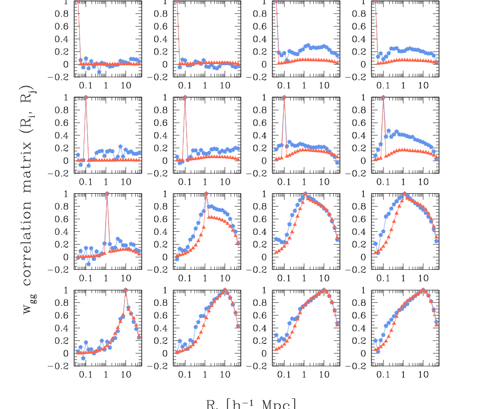
Figure 8: The correlation matrix from Eq. (50) for the projected galaxy correlation function. From top to bottom, the rows present four scales: Ri=0.04,0.1,1,10​h−1​MpcR_{i}=0.04,0.1,1,10\,\,h^{-1}{\rm Mpc}. From left to right, the columns depict the four magnitude bins, as indicated in each panel. The symbols are the same as in the figure above.

6.1 Covariance of the projected correlation function

In Figure 8 we present the errors on the mean projected galaxy correlation function, divided through by the signal, as a function of the transverse scale RR, and for the magnitude bins discussed previously. The blue pentagons in the figure represent the noise-to-signal ratio estimated directly from the N=216N=216 subcubes. The unbiased estimator of the mean and covariance is:

⟨w¯^gg​(Ri)⟩≡1N​∑k=1Nw¯^gg,k​(Ri),\left<\widehat{\widebar{w}}_{\rm gg}(R_{i})\right>\equiv\frac{1}{N}\sum_{k=1}^{N}\widehat{\widebar{w}}_{\rm gg,k}(R_{i}), (48)
Cov⁡[w¯^gg]​(Ri,Rj)\displaystyle{\rm Cov}[\widehat{\widebar{w}}_{\rm gg}](R_{i},R_{j}) ≡1N−1​∑k=1N[w¯^gg,k​(Ri)−⟨w¯^gg​(Ri)⟩]\displaystyle\hskip-17.07182pt\equiv\frac{1}{N-1}\sum_{k=1}^{N}\left[\widehat{\widebar{w}}_{\rm gg,k}(R_{i})-\left<\widehat{\widebar{w}}_{\rm gg}(R_{i})\right>\right]{} (49)
×[w¯^gg,k​(Rj)−⟨w¯^gg​(Rj)⟩],\displaystyle\hskip-17.07182pt\times\left[\widehat{\widebar{w}}_{\rm gg,k}(R_{j})-\left<\widehat{\widebar{w}}_{\rm gg}(R_{j})\right>\right],

where w¯^gg,k\widehat{\widebar{w}}_{\rm gg,k} is the bin-averaged estimate of the projected correlation function from the kkth subcube. The covariance and error on the mean are then simply obtained by further dividing the right-hand side of Eq. (49) by the number of subcubes NN. The red triangles denote the predictions obtained from direct evaluation of Eqs. (26) and (32), where we scaled the variance to the entire MXXL volume.

The theoretical predictions for the brightest galaxies agree extremely well with the measured errors. This owes to the fact that on large scales, R>10​h−1​MpcR>10\,h^{-1}{\rm Mpc}, the errors are determined by the Gaussian part of the variance. On smaller scales these objects are relatively sparse, and so the shot-noise contribution to the variance quickly dominates. Both of these two limits are well characterized by our formula.

For the fainter magnitude bins there is reasonably good agreement between our model and the data on both large (R>10​h−1​MpcR>10\,\,h^{-1}{\rm Mpc}) and small (R<0.1​h−1​MpcR<0.1\,\,h^{-1}{\rm Mpc}) scales. The former is due to the prominence of Gaussian contributions on large scales, whereas the latter is due to the shot noise dominance on small scales. However, on intermediate scales (0.1​h−1​Mpc<R<1​h−1​Mpc0.1\,\,h^{-1}{\rm Mpc}<R<1\,\,h^{-1}{\rm Mpc}), the agreement is not so good, and we see that the data have errors roughly a factor of ∼\sim2 larger than the predictions. This is to be expected, since for these scales the non-Gaussian corrections (e.g. the connected part of the trispectrum and also the bispectrum), which we neglected in deriving Eq. (32) are significant and have the effect of increasing the errors.

To compare the off-diagonal elements of the predicted and measured covariance from Eqs. (32) and (49), we choose to examine the correlation matrix. For any covariance matrix C​[X]\textbf{{C}}[X], the correlation matrix r​[X]\textbf{{r}}[X], can be defined as:

r​[X]i​j=C​[X]i​jC​[X]i​i​C​[X]j​j,r[X]_{ij}=\frac{C[X]_{ij}}{\sqrt{C[X]_{ii}\,C[X]_{jj}}}\ , (50)

where the subscript X{\rm X} is a place-holder for the statistic. The correlation matrix obeys the constraint |r​[X]i​j|≤1,∀i,j\left|r[X]_{ij}\right|\leq 1,\,\forall i,j.

Figure 8 shows four rows of the correlation matrix of r​[w¯^gg]\textbf{{r}}[\widehat{\widebar{w}}_{\rm gg}] at radii (Ri,Rj)(R_{i},R_{j}) as a function of RjR_{j} and at fixed radius RiR_{i}. The fixed scales correspond roughly to Ri=0.04, 0.1, 1, 10​h−1​MpcR_{i}=0.04,\,0.1,\,1,\,10\,\,h^{-1}{\rm Mpc}, and in each panel can be quickly determined by noting that r⁡[w¯^gg]​(Ri=Rj)=1r[\widehat{\widebar{w}}_{\rm gg}](R_{i}=R_{j})=1. From left to right, each column represents a magnitude bin.

There are some notable trends: when the fixed scale RiR_{i} is large (bottom row of the figure), the neighbouring bins of the matrix are significantly correlated, and the strength of the correlations is r⁡[w¯^gg]>0.5r[\widehat{\widebar{w}}_{\rm gg}]>0.5. There is a decrease in the correlation coefficient as one considers brighter magnitude bins. These findings are in good agreement with our Gaussian model. When the fixed scale is small (Ri=0.04)(R_{i}=0.04), for the brighter galaxy bins there is virtually no evidence for bin-to-bin correlations. Again this is consistent with the predictions of our model, and is attributed to the fact that for so few objects the shot-noise errors simply dominate. However, when we consider the intermediate scales (second and third rows of panels in the figure), the model predictions underestimate the bin-to-bin correlations that are exhibited by the data. We interpret this as a sign that the non-Gaussian contributions to the covariance matrix, which we have neglected in our model, are significant. For a more intuitive but less quantitative depiction of the GC correlation matrix, as well as the GGL one and their cross-correlation, we refer the reader to Figures 13-16.

Refer to caption
Figure 9: The noise-to-signal for the stacked tangential shear. The red triangles represent the theory predictions, while the blue pentagons correspond to the simulation measurements.
Refer to caption
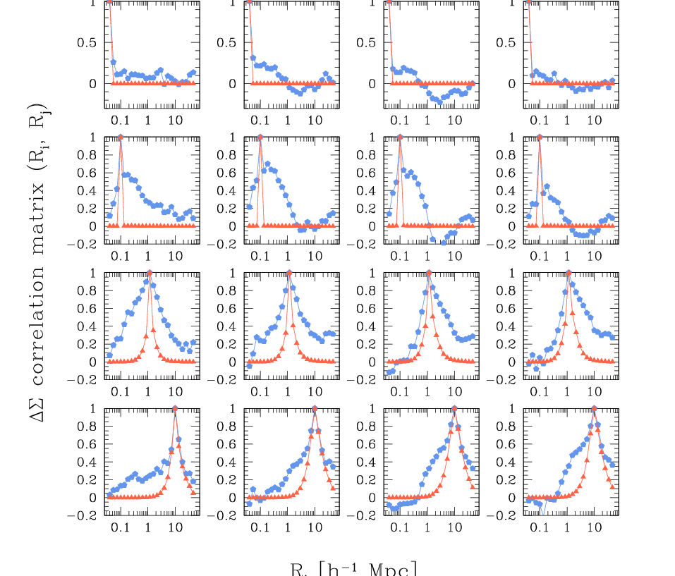
Figure 10: The correlation matrix from Eq. (50) for the stacked tangential shear. Just like in Figure 8, the rows present four scales: Ri=0.04,0.1,1,10​h−1​MpcR_{i}=0.04,0.1,1,10\,\,h^{-1}{\rm Mpc}. From left to right, the columns depict results for increasingly fainter galaxies, as indicated in each panel.

6.2 Covariance of the stacked tangential shear

Figure 10 presents the errors on the mean of the stacked tangential shear as a function of the transverse scale RR. The blue pentagons in the figure represent the noise-to-signal ratio estimated directly from the 216 MXXL-subcubes estimated through:

⟨γ¯^tg​(Ri)⟩≡1Σcrit​1N​∑k=1NΔ​Σ^k​(Ri),\langle\widehat{\widebar{\gamma}}_{t}^{g}(R_{i})\rangle\equiv\frac{1}{\Sigma_{\rm crit}}\frac{1}{N}\sum_{k=1}^{N}\widehat{\Delta\Sigma}_{k}(R_{i}), (51)
Cov⁡[γ¯^tg]​(Ri,Rj)\displaystyle{\rm Cov}[\widehat{\widebar{\gamma}}_{t}^{g}](R_{i},R_{j}) ≡1Σcrit2​1N−1​∑k=1N[Δ​Σ^k​(Ri)−⟨Δ​Σ^k​(Ri)⟩]\displaystyle\hskip-17.07182pt\equiv\frac{1}{\Sigma_{\rm crit}^{2}}\frac{1}{N-1}\hskip-2.84544pt\sum_{k=1}^{N}\left[\widehat{\Delta\Sigma}_{k}(R_{i})-\langle\widehat{\Delta\Sigma}_{k}(R_{i})\rangle\right]{} (52)
×[Δ​Σ^k​(Rj)−⟨Δ​Σ^k​(Rj)⟩],\displaystyle\hskip-17.07182pt\times\left[\widehat{\Delta\Sigma}_{k}(R_{j})-\langle\widehat{\Delta\Sigma}_{k}(R_{j})\rangle\right],

where Δ​Σ^k​(Ri)\widehat{\Delta\Sigma}_{k}(R_{i}) is the estimate of the excess surface density from the kkth subcube.

Let us now turn to the theoretical predictions. We note that Eq. (29) can be rewritten for Δ​Σ\Delta\Sigma at the lens redshift zlz_{l} and using the Limber approximation as done in section §3.2 and Eq. (47). In the following, we shall ignore the shape-noise contribution from Eq. (29), since the latter is not an issue for our measurements. What is an issue however, given that we determine the matter distribution from an NN-body simulation of finite resolution, is the particle shot noise which accompanies 𝒫mm\mathcal{P}_{\rm mm}. We therefore write the final expression for the measured bin-averaged covariance of the excess surface density as:

Cov⁡[Δ​Σ¯^]​(Ri,Rj)\displaystyle{\rm Cov}[\widehat{\widebar{\Delta\Sigma}}](R_{i},R_{j}) =1As​(ρm0)2​∫d2​k⟂(2​π)2​J¯2​(k⟂​Ri)​J¯2​(k⟂​Rj)\displaystyle\hskip-14.22636pt=\frac{1}{A_{s}}(\rho_{m}^{0})^{2}\int\frac{d^{2}k_{\perp}}{(2\pi)^{2}}\widebar{J}_{2}(k_{\perp}R_{i})\widebar{J}_{2}(k_{\perp}R_{j}){} (53)
×{[𝒫mm​(k⟂)+1n¯p]​[𝒫gg​(k⟂)+1n¯g]+𝒫gm2​(k⟂)},\displaystyle\hskip-85.35826pt\times\left\{\left[\mathcal{P}_{\rm mm}(k_{\perp})+\frac{1}{\bar{n}_{p}}\right]\,\left[\mathcal{P}_{\rm gg}(k_{\perp})+\frac{1}{\bar{n}_{g}}\right]+\mathcal{P}_{\rm gm}^{2}(k_{\perp})\right\},

where all the power spectra are taken at redshift zlz_{l}; the transverse area of the survey AsA_{s} was introduced in §3.2; n¯p\bar{n}_{p} and n¯g\bar{n}_{g} are the mean particle and galaxy densities in the simulation. The above covariance has dimension of L−4L^{-4}, as expected.

The theory predictions of Eq. (53) are presented as the red triangles in Figure 10 . As in the case of wggw_{\rm gg}, we see that the agreement between theory and measurements is good on large (R>10​h−1​MpcR>10\,\,h^{-1}{\rm Mpc}) and small (R<0.1​h−1​MpcR<0.1\,\,h^{-1}{\rm Mpc}) scales. However, on intermediate scales the theory underestimates the true errors. We also notice the predictions are increasingly poor for the fainter galaxies. For the brightest galaxies the discrepancy at R∼1​h−1​MpcR\sim 1\,h^{-1}{\rm Mpc} is roughly a factor of ∼2\sim 2, whereas for the faintest galaxies it is roughly ∼3\sim 3. Thus, compared to wggw_{\rm gg}, the predictions for the stacked shear seem worse, even for the shot-noise-dominated brightest galaxies. This suggests that the non-Gaussian contributions to the variance are more important for the stacked tangential shear than for the projected correlation function. However, in a real shear survey this discrepancy may not be so crucial, since the addition of the shape noise term will certainly be a strong source of noise on small-scales. In Appendix §C we present a theoretical estimation of the impact of shape noise on the GGL variance and correlation matrix.

Refer to caption
Figure 11: The cross-correlation matrix of the projected galaxy correlation function and the stacked tangential shear. As in the previous Figures 8 and 10, the rows present four scales: Ri=0.04,0.1,1,10​h−1​MpcR_{i}=0.04,0.1,1,10\,\,h^{-1}{\rm Mpc}. From left to right, the columns depict the galaxy bins with decreasing brightness.
Refer to caption
Figure 12: The cross-correlation matrix of the projected galaxy correlation function and the stacked tangential shear, this time fixing Rj=0.04,0.1,1,10​h−1​MpcR_{j}=0.04,0.1,1,10\,\,h^{-1}{\rm Mpc}.

Figure 10 presents four rows of the correlation matrix of γ¯^tg\widehat{\widebar{\gamma}}^{g}_{t} at {Ri,Rj}\{R_{i},R_{j}\} as a function of RjR_{j} and for fixed RiR_{i}, with the covariance estimated according to Eq. (52). The measurements are represented in the figure as the blue pentagons. The theoretical predictions are obtained by evaluating Eq. (53), and are denoted by the red triangles. The general trends are similar to those found in Figure 8: on small scales (Ri=0.04​h−1​MpcR_{i}=0.04\,\,h^{-1}{\rm Mpc}, i.e. the top row of the figure), the theory and measurements show weak bin-to-bin correlations and the measurements seem somewhat noisy. Qualitatively they are consistent with uncorrelated noise. On large scales (Ri=10.0​h−1​MpcR_{i}=10.0\,\,h^{-1}{\rm Mpc}, i.e. the bottom row of the figure), the measurements show significant bin-to-bin correlations. However, the correlations appear to be somewhat weaker than was found for the projected correlation function for more distant bins. In addition, the Gaussian predictions of our model do not describe these correlations as well as in the case of wggw_{\rm gg}. On intermediate scales, 1<Ri<10​[h−1​Mpc]1<R_{i}<10[\,h^{-1}{\rm Mpc}], the correlations are significantly stronger for all magnitude bins than predicted by our theoretical model. Once again, this suggests that the tangential shear signal is significantly more non-Gaussian on these scales than the projected galaxy correlation function.

6.3 Cross-covariance of the projected correlation function and stacked tangential shear

Refer to caption Refer to caption
Figure 13: The correlation matrix of wggw_{\rm gg} for the four magnitude bins considered. The upper right triangle of the matrix represents the correlation matrix measured from the whole simulation, i.e. the same as in Figure 8. The lower left triangle is the correlation matrix obtained from jackknife samplings of one of the subcubes of the simulation.
Refer to caption Refer to caption
Figure 14: The same as in the figure above, only for the case of Δ​Σ\Delta\Sigma.
Refer to caption Refer to caption
Figure 15: The cross-correlation matrix of wggw_{\rm gg} and Δ​Σ\Delta\Sigma, as computed from the whole MXXL data and presented also in Figures 12 and 12.
Refer to caption Refer to caption
Figure 16: The jackknife cross-correlation matrix of wggw_{\rm gg} and Δ​Σ\Delta\Sigma, estimated from 64 samplings of one of the MXXL subcubes.

In order to perform a joint likelihood analysis of the combination of the projected galaxy correlation function and the stacked tangential shear profile, one would start by writing the joint vector of measurements:

𝐗T=(w¯^gg​(R1)σ⁡[w¯^gg]​(R1),…,w¯^gg​(R𝒩)σ⁡[w¯^gg]​(R𝒩),…​γ¯^tg​(R𝒩)σ⁡[γ¯^tg]​(R𝒩)),{\bf X}^{T}=\left(\frac{\widehat{\widebar{w}}_{\rm gg}(R_{1})}{\sigma[\widehat{\widebar{w}}_{\rm gg}](R_{1})},\dots,\frac{\widehat{\widebar{w}}_{\rm gg}(R_{\mathcal{N}})}{\sigma[\widehat{\widebar{w}}_{\rm gg}](R_{\mathcal{N}})},\dots\frac{\widehat{\widebar{\gamma}}^{g}_{t}(R_{\mathcal{N}})}{\sigma[\widehat{\widebar{\gamma}}^{g}_{t}](R_{\mathcal{N}})}\right)\ , (54)

where we have normalized the measurements by their diagonal errors, so as to obtain dimensionless numbers. 𝒩\mathcal{N} is the number of transverse radial bins. Assuming a Gaussian likelihood, the normalized data would then be written:

log⁡ℒ⁡(𝐗|ϕ)∝∑i,j=1𝒩[Xi−X¯i​(ϕ)]​r​[X]i​j−1​[Xj−X¯j​(ϕ)],\log{\mathcal{L}}({\bf X}|{{\mbox{\boldmath$\phi$}}})\ \propto\sum_{i,j=1}^{\mathcal{N}}[X_{i}-\bar{X}_{i}({{\mbox{\boldmath$\phi$}}})]\ r[X]^{-1}_{ij}\left[X_{j}-\bar{X}_{j}({{\mbox{\boldmath$\phi$}}})\right]\ , (55)

where X¯i​(ϕ)\bar{X}_{i}({\mbox{\boldmath$\phi$}}) is the expectation of the theoretical model, and r​[X]−1\textbf{{r}}[X]^{-1} is the inverse correlation matrix. The correlation matrix is built from four blocks:

r​[X]=(r​[w¯^gg]r​[w¯^gg,γ¯^tg]r​[γ¯^tg,w¯^gg]r​[γ¯^tg])\textbf{{r}}[X]=\left(\begin{array}[]{cc}\textbf{{r}}[\widehat{\widebar{w}}_{\rm gg}]&\textbf{{r}}[\widehat{\widebar{w}}_{\rm gg},\widehat{\widebar{\gamma}}^{g}_{t}]\\ \textbf{{r}}[\widehat{\widebar{\gamma}}^{g}_{t},\widehat{\widebar{w}}_{\rm gg}]&\textbf{{r}}[\widehat{\widebar{\gamma}}^{g}_{t}]\end{array}\right) (56)

where the off-diagonal blocks are simply the transpose of one another. Again we see that |rX|≤1\left|\textbf{{r}}_{X}\right|\leq{1}, i.e. the absolute value of the determinant must be less than unity, through the Cauchy-Schwarz inequality.

Figures 12 and 12 present four rows and columns through the off-diagonal block r​[w¯^gg,γ¯^tg]\textbf{{r}}[\widehat{\widebar{w}}_{\rm gg},\widehat{\widebar{\gamma}}^{g}_{t}] of the full correlation matrix, respectively. Note that unlike the other block matrices, the off-diagonal block is not symmetric, hence the need to examine the columns as well as the rows. Just like before, the blue pentagons denote the measurements from the 216 MXXL subcubes. The cross-covariance was estimated similarly to Eqs. (49) and (52):

Cov⁡[w¯^gg,γ¯^tg]​(Ri,Rj)\displaystyle{\rm Cov}[\widehat{\widebar{w}}_{\rm gg},\widehat{\widebar{\gamma}}_{t}^{g}](R_{i},R_{j}) ≡1Σcrit​1N−1​∑k=1N[w¯^gg,k​(Ri)−⟨w¯^gg​(Ri)⟩]\displaystyle\hskip-17.07182pt\equiv\frac{1}{\Sigma_{\rm crit}}\frac{1}{N-1}\hskip-2.84544pt\sum_{k=1}^{N}\hskip-2.84544pt\left[\widehat{\widebar{w}}_{\rm gg,k}(R_{i})-\left<\widehat{\widebar{w}}_{\rm gg}(R_{i})\right>\right]{} (57)
×[Δ​Σ^k​(Rj)−⟨Δ​Σ^k​(Rj)⟩].\displaystyle\hskip-17.07182pt\times\left[\widehat{\Delta\Sigma}_{k}(R_{j})-\langle\widehat{\Delta\Sigma}_{k}(R_{j})\rangle\right].

Owing to the fact that we use the excess surface mass density as a proxy for tangential shear, we may rewrite Eq. (34) as:

Cov⁡[w¯^gg​(Ri),Δ​Σ¯^​(Rj)]\displaystyle{\rm Cov}[\widehat{\widebar{w}}_{\rm gg}(R_{i}),\widehat{\widebar{\Delta\Sigma}}(R_{j})] =2​ρm0As​∫d2​k⟂(2​π)2​J¯0​(k⟂​Ri)​J¯2​(k⟂​Rj)\displaystyle\hskip-17.07182pt=\frac{2\rho_{m}^{0}}{A_{s}}\int\frac{d^{2}k_{\perp}}{(2\pi)^{2}}\widebar{J}_{0}(k_{\perp}R_{i})\widebar{J}_{2}(k_{\perp}R_{j}){} (58)
×𝒫gm​(k⟂)​[𝒫gg​(k⟂)+1n¯g].\displaystyle\hskip-16.50264pt\times\hskip 2.84544pt\mathcal{P}_{\rm gm}(k_{\perp})\left[\mathcal{P}_{\rm gg}(k_{\perp})+\frac{1}{\bar{n}_{g}}\right].

The theoretical predictions from this expression are presented in Figures 12 and 12 as the red triangles.

On small scales (R<0.1​h−1​MpcR<0.1\,h^{-1}{\rm Mpc}, i.e. the top row of the figures), we see that for all of the magnitude bins considered, the cross-correlation coefficient is small (r<0.2)(r<0.2), and reasonably consistent with the theoretical predictions from Eq. (58). On large scales (R∼10​h−1​MpcR\sim 10\,h^{-1}{\rm Mpc}, i.e. the bottom row in the figures), the cross-correlation coefficient is larger, with r∼0.8r\sim 0.8 for some of the bins. Also, the theoretical predictions are qualitatively in agreement, although the measurements do show a stronger degree of correlation. On intermediate scales (the middle two rows), the measurements show stronger bin-to-bin correlations than predicted by the theory. These correlations on intermediate to large scales are important to include in any joint likelihood analysis of galaxy clustering and galaxy-galaxy lensing. Otherwise, the likelihood search may lead to biased and over-optimistic parameter constraints.

6.4 Testing the jackknife method to estimate covariances

We now want to see how the correlation matrices estimated from the entire MXXL data compare to those evaluated through the jackknife method.

We pick one of the subcubes of the simulation, and generate 64 jackknife samples by removing a region of the subcube and estimating the projected correlation functions from the remaining data. The regions that are removed are in the shape of a rectangular parallelepiped, with the long side aligned with the 𝐳^{\bf\hat{z}} direction of the subcube, i.e. the projection direction, and the shorter sides describing a square in the 𝐱^−𝐲^{\bf\hat{x}}-{\bf\hat{y}} plane. The latter is obtained by dividing the subcube side in 8 equal segments along both 𝐱^{\bf\hat{x}} and 𝐲^{\bf\hat{y}} directions, resulting in 64 adjacent squares. Thus the dimensions of each parallelepiped are 62.5×62.5×500​[h−1​Mpc]362.5\times 62.5\times 500\,[\,h^{-1}{\rm Mpc}]^{3}.

The rest of the calculations follow the same path as detailed in section 5.1. Each jackknife sample requires its own random catalogue. Just as before, the galaxies and dark matter particles are subsampled 32 times, in order to reduce the shot noise and the α\alpha parameter describing the relative density of the simulation and random data. The resulting correlation functions are the average of the 32 subsample measurements. Once the projected correlation functions and excess surface density are computed for each jackknife sample, we combine them to estimate the covariance matrices for Δ​Σ\Delta\Sigma and wggw_{\rm gg}:

Cov⁡[X^,Y^]​(Ri,Rj)=Nsamp−1Nsamp​∑k=1Nsamp[X^k​(Ri)−⟨X^k​(Ri)⟩]\displaystyle{\rm Cov}[\widehat{X},\widehat{Y}](R_{i},R_{j})=\frac{N_{\rm samp}-1}{N_{\rm samp}}\sum_{k=1}^{N_{\rm samp}}\left[\widehat{X}_{k}(R_{i})-\langle\widehat{X}_{k}(R_{i})\rangle\right]{}
×[Y^k​(Rj)−⟨Y^k​(Rj)⟩],\displaystyle\times\left[\widehat{Y}_{k}(R_{j})-\langle\widehat{Y}_{k}(R_{j})\rangle\right]\ ,\hskip 65.44142pt (59)

where Nsamp=64N_{\rm samp}=64; XX and YY stand in for wggw_{\rm gg} or Δ​Σ\Delta\Sigma and the mean is the average of the jackknife samples:

⟨X^​(R)⟩=1Nsamp​∑k=1NsampX^k​(R).\langle\widehat{X}(R)\rangle=\frac{1}{N_{\rm samp}}\sum_{k=1}^{N_{\rm samp}}\widehat{X}_{k}(R)\ .{}

In Figure 13 we present a comparison between our original measurement of the correlation matrix of wggw_{\rm gg} and the one obtained through jackknife resamplings, for the four magnitude bins that we have considered. In each panel, the upper right half depicts the original correlation matrix, while the lower left shows the jackknife result. The agreement is remarkable, with the jackknife result being slightly noisier than the full one. Similarly, Figure 14 shows the same comparison for the excess surface density. Figures 15 and 16 present the original and jackknife cross-correlation matrices respectively. In all figures the jackknife result appears a little more correlated than the original measurement, but in general the agreement is surprising. Although not shown, we have also compared the variance for wggw_{\rm gg} and Δ​Σ\Delta\Sigma: the findings were very similar, with the jackknife variance being a little noisier, but essentially matching the original measurement rather well.

7 Conclusions

In this paper we have explored the required ingredients for performing a joint likelihood analysis of galaxy clustering and galaxy-galaxy lensing. The combination of these probes has the potential to enable simultaneous constraints of the cosmological and galaxy formation model parameters.

In §2, we developed an analytic framework to predict the projected correlation function and the stacked tangential shears of a population of galaxies. We provided both exact and Limber-approximated expressions for the observables in the flat-sky limit. In appendix A we presented the full derivations of the auto- and cross-covariance matrices. In §3 we summarized the results for the case where the underlying density fluctuations are Gaussian and modulated by a shot-noise contribution. The two necessary ingredients for the results of sections §2 and §3 are the galaxy-galaxy and galaxy-matter power spectra or alternatively a model for the bias defined by Eqs (39) and (40).

The theoretical predictions of the models were then tested against measurements from numerical simulations of structure formation. In §4 we provided a brief overview of the MXXL simulation. The galaxy catalogues were generated using the Garching semi-analytic model (SAM) of galaxy formation, which enabled us to compute the uu, gg, rr, ii, zz SDSS absolute magnitudes. As a diagnostic of the SAM galaxies we presented the evolution of the galaxy luminosity function for the five bands. We also explored certain properties of the galaxies as a function of absolute rr band magnitude (MrM_{r}), allowing us to understand the impact of the finite mass resolution of the MXXL simulation on the derived galaxy properties. Through detailed comparison with the Millennium simulation, we determined that resolution effects were qualitatively important only for magnitudes fainter than Mr>−19M_{r}>-19.

In §5 we described our methods for estimating the projected correlations from the MXXL. This required the implementation of fast and efficient algorithms, since the dark matter distribution was represented by over 300 billion dark matter particles and the galaxy catalogue contained more than a billion objects. We thus developed a parallel k-D tree-algorithm for computing the correlation functions of the subsampled matter and galaxy distributions.

We split the galaxy catalogues into four sub-samples based on their MrM_{r}, with the constraint that Mr<−19M_{r}<-19. We also sliced the dark matter and galaxy catalogues into a series of 216 subcubes of volume 500​h−3​Mpc3500\,h^{-3}\,{\rm Mpc}^{3}. As a step towards modelling the GC and GGL signals, we examined the projected galaxy-galaxy and galaxy-matter correlation functions using the estimator proposed by Landy & Szalay (1993). We also computed the bias coefficients as a function of scale from these statistics. We found that on large scales, R>10​h−1​MpcR>10\,h^{-1}{\rm Mpc}, the bias was consistent with being linear and deterministic. On smaller scales, the bias possessed a complex scale dependence, which varied with the magnitude bin through the larger number of satellites and their spatial distribution, as well as the decreasing host mass for the centrals in the fainter bins. We also found that the cross-correlation coefficient was significantly greater than unity on small scales. This could be explained as a consequence of an exclusion effect – no two galaxies may be closer than the sum of their respective virial radii.

We next computed the excess surface-mass density Δ​Σ\Delta\Sigma, which is directly proportional to the tangential shear, and the projected galaxy correlation function for each of the magnitude bins and for each of the 216 subcubes. These were compared to the theoretical predictions in the Limber approximation. The evaluation of the theory required a model for the nonlinear matter power spectrum and the scale-dependence of the bias. For the former we used the halofit code (Smith et al., 2003), and for the latter we took directly the measured bias. We found that on small scales the theory underpredicted the measurements by ≲20%\lesssim 20\% for wggw_{\rm gg} and by ≲30%\lesssim 30\% for Δ​Σ\Delta\Sigma. This was attributed to the diminished accuracy of halofit on small scales. Both functions displayed complicated features for galaxies in the faintest magnitude bin Mr>−20M_{r}>-20. This was again attributed to the increased abundance of satellite galaxies.

In §6 we used the measured estimates of wggw_{\rm gg} and Δ​Σ\Delta\Sigma from the subcubes to construct the auto- and cross- covariance matrices. We found that on large and small scales the errors were reasonably well described by the Gaussian plus shot-noise model. However, on intermediate scales, 0.1<R<10​h−1​Mpc0.1<R<10\,h^{-1}{\rm Mpc}, the measured errors were significantly larger by a factor of ∼2\sim 2–3. This suggests that in order to accurately model the covariance matrix one needs to take account of the non-Gaussian contributions from the bi- and trispectrum. Note that in the case of GGL, the presence of shape noise does alleviate some of the non-Gaussianities on intermediate scales, as shown in Appendix §C.

Importantly, we found that the cross-covariance between wggw_{\rm gg} and Δ​Σ\Delta\Sigma was not zero. The elements of the cross-covariance matrix showed significant bin-to-bin correlations with r∼0.8r\sim 0.8 for some elements on large-scales. This result is important, since in a number of previous analyses neglected the cross-correlation of GC and GGL. Our results suggest that if these correlations are ignored then a standard likelihood analysis would lead to biased and over-optimistic constraints on the parameters of the models.

Finally, we compared the auto- and cross-covariances obtained from the jackknife samplings of one of the subcubes of MXXL with the full simulation covariances. We concluded that the jackknife method is remarkably effective, for both auto- and cross-covariances.

In the future, more work will be required to establish an accurate model of the GC and GGL signals on scales R<5​h−1​MpcR<5\,h^{-1}{\rm Mpc}. We note that, whilst the SAM model of galaxy formation is not to be taken as an exact replica of reality, it nevertheless captures many of the effects that we expect to have to model when constraining model parameters with real data. It will also be important to determine how well the combination of GC and GGL can actually break the degeneracies between the galaxy-formation and cosmological parameters. We shall aim to explore this in a future paper. In the meantime, we note that Eifler et al. (2014) have explored clustering and lensing probe combinations and have included additional non-Gaussian terms in the modelling of the covariances. However, they have assumed a rather simplistic modelling of the galaxy bias, which we showed here it is not the case. This leads us to suspect that their results will be somewhat over-optimistic.

Another possibility is the exploration of the Υ\Upsilon statistic (Baldauf et al., 2010; Mandelbaum et al., 2013), which was developed to remove the complicated scale-dependences of the bias. However, what is not clear, is whether the Υ\Upsilon statistic in combination with galaxy clustering can provide constraints on both the cosmological and galaxy formation model that are competitive with the standard statistics. We leave this for future work.

Acknowledgements

The authors would like thank Simon White, Eiichiro Komatsu, Peter Schneider, and Gary Bernstein for useful discussions, Bruno Henriques for providing the Millennium simulation galaxy catalogue used in Figure 17. We are also grateful to Volker Springel, Adrian Jenkins, Carlos Frenk and Carlton Baugh for their contribution to the MXXL simulation used in this study.The MXXL was carried out on Juropa at the Jülich Supercomputer Centre in Germany. LM thanks MPA for its kind hospitality while this work was being performed. LM was supported by the DFG through the grant MA 4967/1-2. RES acknowledges support from ERC Advanced Grant 246797 GALFORMOD.

References

  • Angulo et al. (2012) Angulo R. E., Springel V., White S. D. M., Jenkins A., Baugh C. M., Frenk C. S., 2012, MNRAS, 426, 2046
  • Angulo et al. (2014) Angulo R. E., White S. D. M., Springel V., Henriques B., 2014, MNRAS, 442, 2131
  • Baldauf et al. (2010) Baldauf T., Smith R. E., Seljak U., Mandelbaum R., 2010, PRD, 81, 063531
  • Bartelmann & Schneider (2001) Bartelmann M., Schneider P., 2001, Phys.  Rep. , 340, 291
  • Blanton et al. (2003) Blanton M. R. et al., 2003, ApJ, 592, 819
  • Brainerd, Blandford & Smail (1996) Brainerd T. G., Blandford R. D., Smail I., 1996, ApJ, 466, 623
  • Cacciato et al. (2009) Cacciato M., van den Bosch F. C., More S., Li R., Mo H. J., Yang X., 2009, MNRAS, 394, 929
  • Cacciato et al. (2013) Cacciato M., van den Bosch F. C., More S., Mo H., Yang X., 2013, MNRAS, 430, 767
  • Dekel & Lahav (1999) Dekel A., Lahav O., 1999, ApJ, 520, 24
  • dell’Antonio & Tyson (1996) dell’Antonio I. P., Tyson J. A., 1996, ApJL, 473, L17
  • Eifler et al. (2014) Eifler T., Krause E., Schneider P., Honscheid K., 2014, MNRAS, 440, 1379
  • Fosalba et al. (2015a) Fosalba P., Crocce M., Gaztañaga E., Castander F. J., 2015a, MNRAS, 448, 2987
  • Fosalba et al. (2015b) Fosalba P., Gaztañaga E., Castander F. J., Crocce M., 2015b, MNRAS, 447, 1319
  • Griffiths et al. (1996) Griffiths R. E., Casertano S., Im M., Ratnatunga K. U., 1996, MNRAS, 282, 1159
  • Guo et al. (2011) Guo Q. et al., 2011, MNRAS, 413, 101
  • Guzik & Seljak (2001) Guzik J., Seljak U., 2001, MNRAS, 321, 439
  • Guzik & Seljak (2002) Guzik J., Seljak U., 2002, MNRAS, 335, 311
  • Hayashi & White (2008) Hayashi E., White S. D. M., 2008, MNRAS, 388, 2
  • Henriques et al. (2012) Henriques B. M. B., White S. D. M., Lemson G., Thomas P. A., Guo Q., Marleau G.-D., Overzier R. A., 2012, MNRAS, 421, 2904
  • Hirata et al. (2004) Hirata C. M. et al., 2004, MNRAS, 353, 529
  • Hoekstra et al. (2002) Hoekstra H., van Waerbeke L., Gladders M. D., Mellier Y., Yee H. K. C., 2002, ApJ, 577, 604
  • Hoekstra, Yee & Gladders (2004) Hoekstra H., Yee H. K. C., Gladders M. D., 2004, ApJ, 606, 67
  • Hudson et al. (2015) Hudson M. J. et al., 2015, MNRAS, 447, 298
  • Hudson et al. (1998) Hudson M. J., Gwyn S. D. J., Dahle H., Kaiser N., 1998, ApJ, 503, 531
  • Jarvis, Bernstein & Jain (2004) Jarvis M., Bernstein G., Jain B., 2004, MNRAS, 352, 338
  • Jeong, Komatsu & Jain (2009) Jeong D., Komatsu E., Jain B., 2009, PRD, 80, 123527
  • Johnston et al. (2007) Johnston D. E. et al., 2007, ArXiv e-prints astro-ph/0709.1159
  • Landy & Szalay (1993) Landy S. D., Szalay A. S., 1993, ApJ, 412, 64
  • Leauthaud et al. (2012) Leauthaud et al., 2012, ApJ, 744, 159
  • Mandelbaum et al. (2006a) Mandelbaum R., Hirata C. M., Broderick T., Seljak U., Brinkmann J., 2006a, MNRAS, 370, 1008
  • Mandelbaum et al. (2005) Mandelbaum R. et al., 2005, MNRAS, 361, 1287
  • Mandelbaum et al. (2006b) Mandelbaum R., Seljak U., Cool R. J., Blanton M., Hirata C. M., Brinkmann J., 2006b, MNRAS, 372, 758
  • Mandelbaum et al. (2006c) Mandelbaum R., Seljak U., Kauffmann G., Hirata C. M., Brinkmann J., 2006c, MNRAS, 368, 715
  • Mandelbaum et al. (2013) Mandelbaum R., Slosar A., Baldauf T., Seljak U., Hirata C. M., Nakajima R., Reyes R., Smith R. E., 2013, MNRAS, 432, 1544
  • McKay et al. (2001) McKay et al., 2001, ArXiv e-prints astro-ph/0108013
  • Miyatake et al. (2013) Miyatake H. et al., 2013, ArXiv e-prints astro-ph/1311.1480
  • Moore et al. (2001) Moore A. W. et al., 2001, in Mining the Sky, Banday A. J., Zaroubi S., Bartelmann M., eds., p. 71
  • More et al. (2014) More S., Miyatake H., Mandelbaum R., Takada M., Spergel D., Brownstein J., Schneider D. P., 2014, ArXiv e-prints astro-ph/1407.1856
  • More et al. (2013) More S., van den Bosch F. C., Cacciato M., More A., Mo H., Yang X., 2013, MNRAS, 430, 747
  • Nakajima et al. (2012) Nakajima R., Mandelbaum R., Seljak U., Cohn J. D., Reyes R., Cool R., 2012, MNRAS, 420, 3240
  • Parker et al. (2007) Parker L. C., Hoekstra H., Hudson M. J., van Waerbeke L., Mellier Y., 2007, ApJ, 669, 21
  • Saghiha et al. (2012) Saghiha H., Hilbert S., Schneider P., Simon P., 2012, A&A, 547, A77
  • Schneider (1998) Schneider P., 1998, ApJ, 498, 43
  • Schneider (2005) Schneider P., 2005, ArXiv e-prints astro-ph/0509252
  • Seljak et al. (2005) Seljak U. et al., 2005, PRD, 71, 043511
  • Seljak & Warren (2004) Seljak U., Warren M. S., 2004, MNRAS, 355, 129
  • Sheldon et al. (2004) Sheldon E. S. et al., 2004, Astronomical Journal, 127, 2544
  • Sheldon et al. (2009a) Sheldon E. S. et al., 2009a, ApJ, 703, 2232
  • Sheldon et al. (2009b) Sheldon E. S. et al., 2009b, ApJ, 703, 2217
  • Smith (2009) Smith R. E., 2009, MNRAS, 400, 851
  • Smith (2012) Smith R. E., 2012, MNRAS, 426, 531
  • Smith & Marian (2014) Smith R. E., Marian L., 2014, ArXiv e-prints astro-ph/1406.1800
  • Smith & Marian (2015) Smith R. E., Marian L., 2015, ArXiv e-prints astro-ph/1503.06830
  • Smith et al. (2003) Smith R. E. et al., 2003, MNRAS, 341, 1311
  • Spergel et al. (2003) Spergel et al., 2003, ApJS, 148, 175
  • Spergel et al. (2007) Spergel et al., 2007, ApJS, 170, 377
  • Springel et al. (2005) Springel V. et al., 2005, Nature, 435, 629
  • Takahashi et al. (2012) Takahashi R., Sato M., Nishimichi T., Taruya A., Oguri M., 2012, ApJ, 761, 152
  • Tyson et al. (1984) Tyson J. A., Valdes F., Jarvis J. F., Mills, Jr. A. P., 1984, ApJL, 281, L59
  • van den Bosch et al. (2013) van den Bosch F. C., More S., Cacciato M., Mo H., Yang X., 2013, MNRAS, 430, 725
  • van Uitert et al. (2011) van Uitert E., Hoekstra H., Velander M., Gilbank D. G., Gladders M. D., Yee H. K. C., 2011, A&A, 534, A14
  • Velander et al. (2014) Velander et al., 2014, MNRAS, 437, 2111
  • Wilson et al. (2001) Wilson G., Kaiser N., Luppino G. A., Cowie L. L., 2001, ApJ, 555, 572
  • Yang, Mo & van den Bosch (2003) Yang X., Mo H. J., van den Bosch F. C., 2003, MNRAS, 339, 1057
  • Yoo et al. (2006) Yoo J., Tinker J. L., Weinberg D. H., Zheng Z., Katz N., Davé R., 2006, ApJ, 652, 26

Appendix A Derivation of the auto- and cross-covariance matrices

A.1 Derivation of the covariance matrix of stacked tangential shear

To simplify the notation, from now on we shall consider that all 2D integrals are implicitly done on the survey area Ωs\Omega_{s} without explicitly stating so in every case.

Using Eq. (11) we write:

⟨γ^tg​(𝜽1)​γ^tg​(𝜽2)⟩\displaystyle\langle\widehat{\gamma}_{t}^{g}({\mbox{\boldmath$\theta$}}_{1})\widehat{\gamma}_{t}^{g}({\mbox{\boldmath$\theta$}}_{2})\rangle =\displaystyle= 1Ng2​∫d2​x​d2​y​∑i,j=1Ng⟨δD​(𝒙−𝒙i)​δD​(𝒚−𝒙j)​γt​(𝒙+𝜽1,𝒙)​γt​(𝒚+𝜽2,𝒚)⟩\displaystyle\frac{1}{N_{g}^{2}}\int d^{2}x\,d^{2}y\sum_{i,j=1}^{N_{g}}\langle\delta_{D}({\mbox{\boldmath$x$}}-{\mbox{\boldmath$x$}}_{i})\delta_{D}({\mbox{\boldmath$y$}}-{\mbox{\boldmath$x$}}_{j})\gamma_{t}({\mbox{\boldmath$x$}}+{\mbox{\boldmath$\theta$}}_{1};{\mbox{\boldmath$x$}})\gamma_{t}({\mbox{\boldmath$y$}}+{\mbox{\boldmath$\theta$}}_{2};{\mbox{\boldmath$y$}})\rangle (60)
=\displaystyle= 1Ng2​[∫d2​x​⟨ng​(𝒙)​γt​(𝒙+𝜽1,𝒙)​γt​(𝒙+𝜽2,𝒙)⟩+∫d2​x​d2​y​⟨ng​(𝒙)​ng​(𝒚)​γt​(𝒙+𝜽1,𝒙)​γt​(𝒚+𝜽2,𝒚)⟩].\displaystyle\frac{1}{N_{g}^{2}}\left[\int d^{2}x\langle n_{g}({\mbox{\boldmath$x$}})\gamma_{t}({\mbox{\boldmath$x$}}+{\mbox{\boldmath$\theta$}}_{1};{\mbox{\boldmath$x$}})\gamma_{t}({\mbox{\boldmath$x$}}+{\mbox{\boldmath$\theta$}}_{2};{\mbox{\boldmath$x$}})\rangle+\int d^{2}x\,d^{2}y\,\langle n_{g}({\mbox{\boldmath$x$}})n_{g}({\mbox{\boldmath$y$}})\gamma_{t}({\mbox{\boldmath$x$}}+{\mbox{\boldmath$\theta$}}_{1};{\mbox{\boldmath$x$}})\gamma_{t}({\mbox{\boldmath$y$}}+{\mbox{\boldmath$\theta$}}_{2};{\mbox{\boldmath$y$}})\rangle\right].

In the above double sum, the special case where i=ji=j gives rise to the 3-point function ⟨ng​(𝒙)​γt​(𝒙+𝜽1,𝒙)​γt​(𝒙+𝜽2,𝒙)⟩=n¯g​[⟨γt​(𝒙+𝜽1,𝒙)​γt​(𝒙+𝜽2,𝒙)⟩+⟨δg​(𝒙)​γt​(𝒙+𝜽1,𝒙)​γt​(𝒙+𝜽2,𝒙)⟩]\langle n_{g}({\mbox{\boldmath$x$}})\gamma_{t}({\mbox{\boldmath$x$}}+{\mbox{\boldmath$\theta$}}_{1};{\mbox{\boldmath$x$}})\gamma_{t}({\mbox{\boldmath$x$}}+{\mbox{\boldmath$\theta$}}_{2};{\mbox{\boldmath$x$}})\rangle=\bar{n}_{g}[\langle\gamma_{t}({\mbox{\boldmath$x$}}+{\mbox{\boldmath$\theta$}}_{1};{\mbox{\boldmath$x$}})\gamma_{t}({\mbox{\boldmath$x$}}+{\mbox{\boldmath$\theta$}}_{2};{\mbox{\boldmath$x$}})\rangle+\langle\delta_{g}({\mbox{\boldmath$x$}})\gamma_{t}({\mbox{\boldmath$x$}}+{\mbox{\boldmath$\theta$}}_{1};{\mbox{\boldmath$x$}})\gamma_{t}({\mbox{\boldmath$x$}}+{\mbox{\boldmath$\theta$}}_{2};{\mbox{\boldmath$x$}})\rangle]. Similarly, the case where i≠ji\neq j yields a 4-point function which can be expressed as ⟨ng​(𝒙)​ng​(𝒚)​γt​(𝒙+𝜽1,𝒙)​γt​(𝒚+𝜽2,𝒚)⟩=n¯g2​{⟨γt​(𝒙+𝜽1,𝒙)​γt​(𝒚+𝜽2,𝒚)⟩+⟨δg​(𝒙)​δg​(𝒚)​γt​(𝒙+𝜽1,𝒙)​γt​(𝒚+𝜽2,𝒚)⟩+⟨δg​(𝒙)​γt​(𝒙+𝜽1,𝒙)​γt​(𝒚+𝜽2,𝒚)⟩+⟨δg​(𝒚)​γt​(𝒙+𝜽1,𝒙)​γt​(𝒚+𝜽2,𝒚)⟩}.\langle n_{g}({\mbox{\boldmath$x$}})n_{g}({\mbox{\boldmath$y$}})\gamma_{t}({\mbox{\boldmath$x$}}+{\mbox{\boldmath$\theta$}}_{1};{\mbox{\boldmath$x$}})\gamma_{t}({\mbox{\boldmath$y$}}+{\mbox{\boldmath$\theta$}}_{2};{\mbox{\boldmath$y$}})\rangle=\bar{n}_{g}^{2}\,\{\langle\gamma_{t}({\mbox{\boldmath$x$}}+{\mbox{\boldmath$\theta$}}_{1};{\mbox{\boldmath$x$}})\gamma_{t}({\mbox{\boldmath$y$}}+{\mbox{\boldmath$\theta$}}_{2};{\mbox{\boldmath$y$}})\rangle+\langle\delta_{g}({\mbox{\boldmath$x$}})\delta_{g}({\mbox{\boldmath$y$}})\gamma_{t}({\mbox{\boldmath$x$}}+{\mbox{\boldmath$\theta$}}_{1};{\mbox{\boldmath$x$}})\gamma_{t}({\mbox{\boldmath$y$}}+{\mbox{\boldmath$\theta$}}_{2};{\mbox{\boldmath$y$}})\rangle+\langle\delta_{g}({\mbox{\boldmath$x$}})\gamma_{t}({\mbox{\boldmath$x$}}+{\mbox{\boldmath$\theta$}}_{1};{\mbox{\boldmath$x$}})\gamma_{t}({\mbox{\boldmath$y$}}+{\mbox{\boldmath$\theta$}}_{2};{\mbox{\boldmath$y$}})\rangle+\langle\delta_{g}({\mbox{\boldmath$y$}})\gamma_{t}({\mbox{\boldmath$x$}}+{\mbox{\boldmath$\theta$}}_{1};{\mbox{\boldmath$x$}})\gamma_{t}({\mbox{\boldmath$y$}}+{\mbox{\boldmath$\theta$}}_{2};{\mbox{\boldmath$y$}})\rangle\}. Since this work assumes the Gaussianity of all cosmological fields, we ignore their odd-point functions, as well as the connected functions. After decomposing the 4-point function in the above relation in products of 2-point functions, in accordance to Wick’s theorem, we write Eq. (60) as

⟨γ^tg​(𝜽1)​γ^tg​(𝜽2)⟩\displaystyle\langle\widehat{\gamma}_{t}^{g}({\mbox{\boldmath$\theta$}}_{1})\widehat{\gamma}_{t}^{g}({\mbox{\boldmath$\theta$}}_{2})\rangle =\displaystyle= 1Ωs2{1n¯g∫d2x⟨γt(𝒙+𝜽1;𝒙)γt(𝒙+𝜽2;𝒙)⟩+∫d2xd2y[⟨γt(𝒙+𝜽1;𝒙)γt(𝒚+𝜽2;𝒚)⟩\displaystyle\frac{1}{\Omega_{s}^{2}}\left\{\frac{1}{\bar{n}_{g}}\int d^{2}x\,\langle\gamma_{t}({\mbox{\boldmath$x$}}+{\mbox{\boldmath$\theta$}}_{1};{\mbox{\boldmath$x$}})\gamma_{t}({\mbox{\boldmath$x$}}+{\mbox{\boldmath$\theta$}}_{2};{\mbox{\boldmath$x$}})\rangle+\int d^{2}x\,d^{2}y\left[\langle\gamma_{t}({\mbox{\boldmath$x$}}+{\mbox{\boldmath$\theta$}}_{1};{\mbox{\boldmath$x$}})\gamma_{t}({\mbox{\boldmath$y$}}+{\mbox{\boldmath$\theta$}}_{2};{\mbox{\boldmath$y$}})\rangle\right.\right. (61)
+\displaystyle+ ⟨δg​(𝒙)​δg​(𝒚)⟩​⟨γt​(𝒙+𝜽1,𝒙)​γt​(𝒚+𝜽2,𝒚)⟩+⟨δg​(𝒙)​γt​(𝒙+𝜽1,𝒙)⟩​⟨δg​(𝒚)​γt​(𝒚+𝜽2,𝒚)⟩\displaystyle\left.\left.\langle\delta_{g}({\mbox{\boldmath$x$}})\delta_{g}({\mbox{\boldmath$y$}})\rangle\langle\gamma_{t}({\mbox{\boldmath$x$}}+{\mbox{\boldmath$\theta$}}_{1};{\mbox{\boldmath$x$}})\gamma_{t}({\mbox{\boldmath$y$}}+{\mbox{\boldmath$\theta$}}_{2};{\mbox{\boldmath$y$}})\rangle+\langle\delta_{g}({\mbox{\boldmath$x$}})\gamma_{t}({\mbox{\boldmath$x$}}+{\mbox{\boldmath$\theta$}}_{1};{\mbox{\boldmath$x$}})\rangle\langle\delta_{g}({\mbox{\boldmath$y$}})\gamma_{t}({\mbox{\boldmath$y$}}+{\mbox{\boldmath$\theta$}}_{2};{\mbox{\boldmath$y$}})\rangle\right.\right.
+\displaystyle+ ⟨δg(𝒙)γt(𝒚+𝜽2;𝒚)⟩⟨δg(𝒚)γt(𝒙+𝜽1;𝒙)⟩]}.\displaystyle\left.\left.\langle\delta_{g}({\mbox{\boldmath$x$}})\gamma_{t}({\mbox{\boldmath$y$}}+{\mbox{\boldmath$\theta$}}_{2};{\mbox{\boldmath$y$}})\rangle\langle\delta_{g}({\mbox{\boldmath$y$}})\gamma_{t}({\mbox{\boldmath$x$}}+{\mbox{\boldmath$\theta$}}_{1};{\mbox{\boldmath$x$}})\rangle\right]\frac{}{}\right\}.

We now proceed to the computation of each of the five terms in Eq. (61), omitting for now the inverse square of the survey area that multiplies the whole covariance. Our final goal is in fact the azimuthal average of the covariance in Eq. (27). We first introduce the shape-noise contribution to the covariance of the tangential shear at 𝜽1,𝜽2{\mbox{\boldmath$\theta$}}_{1},{\mbox{\boldmath$\theta$}}_{2} with respect to the origins 𝜽01,𝜽02{\mbox{\boldmath$\theta$}}_{01},{\mbox{\boldmath$\theta$}}_{02}:

⟨γt​(𝜽1,𝜽01)​γt​(𝜽2,𝜽02)⟩=σγ22​n¯s​cos⁡[2​(ϕ𝜽1−𝜽01−ϕ𝜽2−𝜽02)]​δD​(𝜽1−𝜽2),\langle\gamma_{t}({\mbox{\boldmath$\theta$}}_{1};{\mbox{\boldmath$\theta$}}_{01})\gamma_{t}({\mbox{\boldmath$\theta$}}_{2};{\mbox{\boldmath$\theta$}}_{02})\rangle=\frac{\sigma_{\gamma}^{2}}{2\bar{n}_{s}}\cos[2(\phi_{{\mbox{\boldmath$\theta$}}_{1}-{\mbox{\boldmath$\theta$}}_{01}}-\phi_{{\mbox{\boldmath$\theta$}}_{2}-{\mbox{\boldmath$\theta$}}_{02}})]\,\delta_{D}({\mbox{\boldmath$\theta$}}_{1}-{\mbox{\boldmath$\theta$}}_{2}), (62)

where we defined σγ2/2≡σγ12=σγ22\sigma_{\gamma}^{2}/2\equiv\sigma_{\gamma_{1}}^{2}=\sigma_{\gamma_{2}}^{2} as the variance per shear component in the measurement of one source galaxy. We assume the source galaxies to have a mean angular density of n¯s\bar{n}_{s}. In the above we also assumed that the shape noise does not correlate different positions in the source plane, i.e. we ignore for example the effect of intrinsic alignments which might introduce precisely such correlations.

Starting with the first term, we employ Eq. (6) to write:

T1​(𝜽1,𝜽2)\displaystyle T_{1}({\mbox{\boldmath$\theta$}}_{1},{\mbox{\boldmath$\theta$}}_{2}) ≡\displaystyle\equiv 1n¯g​∫d2​x​⟨γt​(𝒙+𝜽1,𝒙)​γt​(𝒙+𝜽2,𝒙)⟩=Ωsn¯g​⟨γt​(𝜽1,𝟎)​γt​(𝜽2,𝟎)⟩\displaystyle\frac{1}{\bar{n}_{g}}\int d^{2}x\,\langle\gamma_{t}({\mbox{\boldmath$x$}}+{\mbox{\boldmath$\theta$}}_{1};{\mbox{\boldmath$x$}})\gamma_{t}({\mbox{\boldmath$x$}}+{\mbox{\boldmath$\theta$}}_{2};{\mbox{\boldmath$x$}})\rangle=\frac{\Omega_{s}}{\bar{n}_{g}}\langle\gamma_{t}({\mbox{\boldmath$\theta$}}_{1};{\bf 0})\gamma_{t}({\mbox{\boldmath$\theta$}}_{2};{\bf 0})\rangle
=\displaystyle= Ωsn¯g​[∫d2​l(2​π)2​cos⁡[2​(ϕ𝜽1−ϕ𝒍)]​cos⁡[2​(ϕ𝜽2−ϕ𝒍)]​𝒞κ​κ​(l)+σγ22​n¯s​cos⁡[2​(ϕ𝜽1−ϕ𝜽2)]​δD​(𝜽1−𝜽2)],\displaystyle\frac{\Omega_{s}}{\bar{n}_{g}}\left[\int\frac{d^{2}l}{(2\pi)^{2}}\cos[2(\phi_{{\mbox{\boldmath$\theta$}}_{1}}-\phi_{{\mbox{\boldmath$l$}}})]\cos[2(\phi_{{\mbox{\boldmath$\theta$}}_{2}}-\phi_{{\mbox{\boldmath$l$}}})]\mathcal{C}_{\kappa\kappa}(l)+\frac{\sigma_{\gamma}^{2}}{2\bar{n}_{s}}\cos[2(\phi_{{\mbox{\boldmath$\theta$}}_{1}}-\phi_{{\mbox{\boldmath$\theta$}}_{2}})]\delta_{D}({\mbox{\boldmath$\theta$}}_{1}-{\mbox{\boldmath$\theta$}}_{2})\right],

Writing that δD​(𝜽1−𝜽2)=δD​(θ1−θ2)​δD​(ϕ𝜽1−ϕ𝜽2)/θ1\delta_{D}({\mbox{\boldmath$\theta$}}_{1}-{\mbox{\boldmath$\theta$}}_{2})=\delta_{D}(\theta_{1}-\theta_{2})\delta_{D}(\phi_{{\mbox{\boldmath$\theta$}}_{1}}-\phi_{{\mbox{\boldmath$\theta$}}_{2}})/\theta_{1}, we compute the azimuthal average of the above equation using Eqs. (7) and (9). Thus the first term of the covariance of the stacked shear estimator is:

T1,a​(θ1,θ2)≡∫02​πd​ϕ𝜽12​π​d​ϕ𝜽22​π​T1​(𝜽1,𝜽2)\displaystyle T_{1,a}(\theta_{1},\theta_{2})\equiv\int_{0}^{2\pi}\frac{d\phi_{{\mbox{\boldmath$\theta$}}_{1}}}{2\pi}\frac{d\phi_{{\mbox{\boldmath$\theta$}}_{2}}}{2\pi}T_{1}({\mbox{\boldmath$\theta$}}_{1},{\mbox{\boldmath$\theta$}}_{2}) =\displaystyle= Ωsn¯g​[∫d2​l(2​π)2​𝒞κ​κ​(l)​J2​(l​θ1)​J2​(l​θ2)+σγ22​n¯s​δD​(θ1−θ2)2​π​θ1]\displaystyle\frac{\Omega_{s}}{\bar{n}_{g}}\left[\int\frac{d^{2}l}{(2\pi)^{2}}\mathcal{C}_{\kappa\kappa}(l)J_{2}(l\theta_{1})J_{2}(l\theta_{2})+\frac{\sigma_{\gamma}^{2}}{2\bar{n}_{s}}\frac{\delta_{D}(\theta_{1}-\theta_{2})}{2\pi\theta_{1}}\right] (63)
=\displaystyle= Ωsn¯g​∫d2​l(2​π)2​[𝒞κ​κ​(l)+σγ22​n¯s]​J2​(l​θ1)​J2​(l​θ2),\displaystyle\frac{\Omega_{s}}{\bar{n}_{g}}\int\frac{d^{2}l}{(2\pi)^{2}}\left[\mathcal{C}_{\kappa\kappa}(l)+\frac{\sigma_{\gamma}^{2}}{2\bar{n}_{s}}\right]J_{2}(l\theta_{1})J_{2}(l\theta_{2}),

where we have put the shape noise term in a similar form to the rest of the first term by using the Bessel identity:

δD​(θ1−θ2)2​π​θ1=∫d2​l(2​π)2​J2​(l​θ1)​J2​(l​θ2).\frac{\delta_{D}(\theta_{1}-\theta_{2})}{2\pi\theta_{1}}=\int\frac{d^{2}l}{(2\pi)^{2}}J_{2}(l\theta_{1})J_{2}(l\theta_{2}).

The second term of the covariance matrix is a constant, equal in fact to 00. This can be seen through a simple change of variables: 𝒙′=𝒙+𝜽1{\mbox{\boldmath$x$}}^{\prime}={\mbox{\boldmath$x$}}+{\mbox{\boldmath$\theta$}}_{1} and 𝒚′=𝒚+𝜽2{\mbox{\boldmath$y$}}^{\prime}={\mbox{\boldmath$y$}}+{\mbox{\boldmath$\theta$}}_{2} which leaves the Jacobian unchanged, d2​x′=d2​x,d2​y′=d2​yd^{2}x^{\prime}=d^{2}x,\,d^{2}y^{\prime}=d^{2}y. Relabelling 𝒙′=𝒙{\mbox{\boldmath$x$}}^{\prime}={\mbox{\boldmath$x$}} and 𝒚′=𝒚{\mbox{\boldmath$y$}}^{\prime}={\mbox{\boldmath$y$}}, we write:

T2​(𝜽1,𝜽2)\displaystyle T_{2}({\mbox{\boldmath$\theta$}}_{1},{\mbox{\boldmath$\theta$}}_{2}) ≡\displaystyle\equiv ∫d2​x​d2​y​⟨γt​(𝒙+𝜽1,𝒙)​γt​(𝒚+𝜽2,𝒚)⟩\displaystyle\int d^{2}x\,d^{2}y\,\langle\gamma_{t}({\mbox{\boldmath$x$}}+{\mbox{\boldmath$\theta$}}_{1};{\mbox{\boldmath$x$}})\gamma_{t}({\mbox{\boldmath$y$}}+{\mbox{\boldmath$\theta$}}_{2};{\mbox{\boldmath$y$}})\rangle (64)
=\displaystyle= ∫d2​x​∫d2​y​⟨γt​(𝒙,𝒙−𝜽1)​γt​(𝒚,𝒚−𝜽2)⟩=⟨∫d2​x​γt​(𝒙,𝒙−𝜽1)​∫d2​y​γt​(𝒚,𝒚−𝜽2)⟩=0.\displaystyle\int d^{2}x\int d^{2}y\,\langle\gamma_{t}({\mbox{\boldmath$x$}};{\mbox{\boldmath$x$}}-{\mbox{\boldmath$\theta$}}_{1})\gamma_{t}({\mbox{\boldmath$y$}};{\mbox{\boldmath$y$}}-{\mbox{\boldmath$\theta$}}_{2})\rangle=\langle\int d^{2}x\,\gamma_{t}({\mbox{\boldmath$x$}};{\mbox{\boldmath$x$}}-{\mbox{\boldmath$\theta$}}_{1})\int d^{2}y\,\gamma_{t}({\mbox{\boldmath$y$}};{\mbox{\boldmath$y$}}-{\mbox{\boldmath$\theta$}}_{2})\rangle=0.

In the above we have used the ergodic theorem and implicitly assumed that the survey area is sufficiently large so that the tangential shear integrated over it behaves like the ensemble average of the tangential shear, and is therefore equal to 0.

We now turn our attention to the calculation of the third term of Eq. (61), henceforth denoted as T3T_{3}.

T3​(𝜽1,𝜽2)≡∫d2​x​d2​y​⟨δg​(𝒙)​δg​(𝒚)⟩​⟨γt​(𝒙+𝜽1,𝒙)​γt​(𝒚+𝜽2,𝒚)⟩.T_{3}({\mbox{\boldmath$\theta$}}_{1},{\mbox{\boldmath$\theta$}}_{2})\equiv\int d^{2}x\,d^{2}y\,\langle\delta_{g}({\mbox{\boldmath$x$}})\delta_{g}({\mbox{\boldmath$y$}})\rangle\langle\gamma_{t}({\mbox{\boldmath$x$}}+{\mbox{\boldmath$\theta$}}_{1};{\mbox{\boldmath$x$}})\gamma_{t}({\mbox{\boldmath$y$}}+{\mbox{\boldmath$\theta$}}_{2};{\mbox{\boldmath$y$}})\rangle. (65)

Using the invariance under translation due to the homogeneity of the Universe, we have that ⟨δg​(𝒙)​δg​(𝒚)⟩=⟨δg​(𝒙−𝒚)​δg​(𝟎)⟩\langle\delta_{g}({\mbox{\boldmath$x$}})\delta_{g}({\mbox{\boldmath$y$}})\rangle=\langle\delta_{g}({\mbox{\boldmath$x$}}-{\mbox{\boldmath$y$}})\delta_{g}({\bf 0})\rangle, and ⟨γt​(𝒙+𝜽1,𝒙)​γt​(𝒚+𝜽2,𝒚)⟩=⟨γt​(𝒙−𝒚+𝜽1,𝒙−𝒚)​γt​(𝜽2,𝟎)⟩\langle\gamma_{t}({\mbox{\boldmath$x$}}+{\mbox{\boldmath$\theta$}}_{1};{\mbox{\boldmath$x$}})\gamma_{t}({\mbox{\boldmath$y$}}+{\mbox{\boldmath$\theta$}}_{2};{\mbox{\boldmath$y$}})\rangle=\langle\gamma_{t}({\mbox{\boldmath$x$}}-{\mbox{\boldmath$y$}}+{\mbox{\boldmath$\theta$}}_{1};{\mbox{\boldmath$x$}}-{\mbox{\boldmath$y$}})\gamma_{t}({\mbox{\boldmath$\theta$}}_{2};{\bf 0})\rangle. Changing variables 𝒙′=𝒙−𝒚{\mbox{\boldmath$x$}}^{\prime}={\mbox{\boldmath$x$}}-{\mbox{\boldmath$y$}} and relabelling 𝒙′=𝒙{\mbox{\boldmath$x$}}^{\prime}={\mbox{\boldmath$x$}}, we write

T3​(𝜽1,𝜽2)=Ωs​∫d2​x​⟨δg​(𝒙)​δg​(𝟎)⟩​⟨γt​(𝒙+𝜽1,𝒙)​γt​(𝜽2,𝟎)⟩T_{3}({\mbox{\boldmath$\theta$}}_{1},{\mbox{\boldmath$\theta$}}_{2})=\Omega_{s}\int d^{2}x\,\langle\delta_{g}({\mbox{\boldmath$x$}})\delta_{g}({\bf 0})\rangle\langle\gamma_{t}({\mbox{\boldmath$x$}}+{\mbox{\boldmath$\theta$}}_{1};{\mbox{\boldmath$x$}})\gamma_{t}({\mbox{\boldmath$\theta$}}_{2};{\bf 0})\rangle (66)

Note that T3T_{3} also has a contribution from shape noise, which we address below. We shall evaluate Eq. (66) in Fourier space. The Fourier transforms of the shear and galaxy density fluctuations are written as four integrals over the wave vectors which can be reduced to two integrals, by using the definitions of the convergence and galaxy power spectra in Eq. (13):

T3​(𝜽1,𝜽2)\displaystyle T_{3}({\mbox{\boldmath$\theta$}}_{1},{\mbox{\boldmath$\theta$}}_{2}) =\displaystyle= Ωs{∫d2​l1(2​π)2d2​l2(2​π)2𝒞g​g(l1)𝒞κ​κ(l2)ei​𝒍2⋅(𝜽1−𝜽2)cos[2(ϕ𝜽1−ϕ𝒍2)]cos[2(ϕ𝜽2−ϕ𝒍2)]∫d2xei​𝒙⋅(𝒍1+𝒍2)\displaystyle\Omega_{s}\left\{\int\frac{d^{2}l_{1}}{(2\pi)^{2}}\frac{d^{2}l_{2}}{(2\pi)^{2}}\mathcal{C}_{gg}(l_{1})\,\mathcal{C}_{\kappa\kappa}(l_{2})\,e^{i\,{\mbox{\boldmath$l$}}_{2}\cdot({\mbox{\boldmath$\theta$}}_{1}-{\mbox{\boldmath$\theta$}}_{2})}\cos[2(\phi_{{\mbox{\boldmath$\theta$}}_{1}}-\phi_{{\mbox{\boldmath$l$}}_{2}})]\cos[2(\phi_{{\mbox{\boldmath$\theta$}}_{2}}-\phi_{{\mbox{\boldmath$l$}}_{2}})]\int d^{2}x\,e^{i\,{\mbox{\boldmath$x$}}\cdot({\mbox{\boldmath$l$}}_{1}+{\mbox{\boldmath$l$}}_{2})}\right. (67)
+\displaystyle+ σγ22​n¯s∫d2x⟨δg(𝒙)δg(𝟎)⟩cos[2(ϕ𝜽1−ϕ𝜽2)]δD(𝒙+𝜽1−𝜽2)}\displaystyle\left.\frac{\sigma_{\gamma}^{2}}{2\bar{n}_{s}}\,\int d^{2}x\,\langle\delta_{g}({\mbox{\boldmath$x$}})\delta_{g}({\bf 0})\rangle\,\cos[2(\phi_{{\mbox{\boldmath$\theta$}}_{1}}-\phi_{{\mbox{\boldmath$\theta$}}_{2}})]\,\delta_{D}({\mbox{\boldmath$x$}}+{\mbox{\boldmath$\theta$}}_{1}-{\mbox{\boldmath$\theta$}}_{2})\right\}
=\displaystyle= Ωs{∫d2​l(2​π)2𝒞g​g(l)𝒞κ​κ(l)ei​𝒍⋅(𝜽1−𝜽2)cos[2(ϕ𝜽1−ϕ𝒍)]cos[2(ϕ𝜽2−ϕ𝒍)]\displaystyle\Omega_{s}\left\{\int\frac{d^{2}l}{(2\pi)^{2}}\mathcal{C}_{gg}(l)\,\mathcal{C}_{\kappa\kappa}(l)\,e^{i\,{\mbox{\boldmath$l$}}\cdot({\mbox{\boldmath$\theta$}}_{1}-{\mbox{\boldmath$\theta$}}_{2})}\cos[2(\phi_{{\mbox{\boldmath$\theta$}}_{1}}-\phi_{{\mbox{\boldmath$l$}}})]\cos[2(\phi_{{\mbox{\boldmath$\theta$}}_{2}}-\phi_{{\mbox{\boldmath$l$}}})]\right.
+\displaystyle+ σγ22​n¯s∫d2​l(2​π)2𝒞g​g(l)ei​𝒍⋅(𝜽2−𝜽1)cos[2(ϕ𝜽1−ϕ𝜽2)]}.\displaystyle\left.\frac{\sigma_{\gamma}^{2}}{2\bar{n}_{s}}\int\frac{d^{2}l}{(2\pi)^{2}}\mathcal{C}_{gg}(l)e^{i\,{\mbox{\boldmath$l$}}\cdot({\mbox{\boldmath$\theta$}}_{2}-{\mbox{\boldmath$\theta$}}_{1})}\cos[2(\phi_{{\mbox{\boldmath$\theta$}}_{1}}-\phi_{{\mbox{\boldmath$\theta$}}_{2}})]\right\}.

We now calculate the azimuthal average of this term, using just as before Eq. (9). For the shape noise term we also change variables to ϕ𝜽1,2′=ϕ𝜽1,2−ϕ𝒍\phi^{\prime}_{{\mbox{\boldmath$\theta$}}_{1,2}}=\phi_{{\mbox{\boldmath$\theta$}}_{1,2}}-\phi_{{\mbox{\boldmath$l$}}}.

T3,a​(θ1,θ2)\displaystyle T_{3,a}(\theta_{1},\theta_{2}) ≡\displaystyle\equiv ∫02​πd​ϕ𝜽12​πd​ϕ𝜽22​πT3(𝜽1,𝜽2)=Ωs{∫d2​l(2​π)2𝒞g​g(l)𝒞κ​κ(l)J2(lθ1)J2(lθ2)\displaystyle\int_{0}^{2\pi}\frac{d\phi_{{\mbox{\boldmath$\theta$}}_{1}}}{2\pi}\frac{d\phi_{{\mbox{\boldmath$\theta$}}_{2}}}{2\pi}T_{3}({\mbox{\boldmath$\theta$}}_{1},{\mbox{\boldmath$\theta$}}_{2})=\Omega_{s}\left\{\int\frac{d^{2}l}{(2\pi)^{2}}\mathcal{C}_{gg}(l)\,\mathcal{C}_{\kappa\kappa}(l)J_{2}(l\theta_{1})J_{2}(l\theta_{2})\right. (68)
+\displaystyle+ σγ22​n¯s∫d2​l(2​π)2𝒞g​g(l)∫d​ϕ𝜽1′2​πd​ϕ𝜽2′2​πei⁡[l​θ2​cos⁡(ϕ𝜽2′)−l​θ1​cos⁡(ϕ𝜽1′)]cos[2(ϕ𝜽1′−ϕ𝜽2′)]}\displaystyle\left.\frac{\sigma_{\gamma}^{2}}{2\bar{n}_{s}}\int\frac{d^{2}l}{(2\pi)^{2}}\mathcal{C}_{gg}(l)\int\frac{d\phi^{\prime}_{{\mbox{\boldmath$\theta$}}_{1}}}{2\pi}\frac{d\phi^{\prime}_{{\mbox{\boldmath$\theta$}}_{2}}}{2\pi}\,e^{i\,[l\theta_{2}\cos(\phi^{\prime}_{{\mbox{\boldmath$\theta$}}_{2}})-l\theta_{1}\cos(\phi^{\prime}_{{\mbox{\boldmath$\theta$}}_{1}})]}\cos[2(\phi^{\prime}_{{\mbox{\boldmath$\theta$}}_{1}}-\phi^{\prime}_{{\mbox{\boldmath$\theta$}}_{2}})]\right\}
=\displaystyle= Ωs​{∫d2​l(2​π)2​𝒞g​g​(l)​[𝒞κ​κ​(l)+σγ22​n¯s]​J2​(l​θ1)​J2​(l​θ2)}.\displaystyle\Omega_{s}\left\{\int\frac{d^{2}l}{(2\pi)^{2}}\mathcal{C}_{gg}(l)\,\left[\mathcal{C}_{\kappa\kappa}(l)+\frac{\sigma_{\gamma}^{2}}{2\bar{n}_{s}}\right]J_{2}(l\theta_{1})J_{2}(l\theta_{2})\right\}.

Moving on to the fourth term of Eq. (61), we take advantage of the homogeneity of the Universe and of Eq. (14) to write:

T4​(𝜽1,𝜽2)≡∫d2​x​d2​y​⟨δg​(𝒙)​γt​(𝒙+𝜽1,𝒙)⟩​⟨δg​(𝒚)​γt​(𝒚+𝜽2,𝒚)⟩=Ωs2​⟨δg​(𝟎)​γt​(𝜽1,𝟎)⟩​⟨δg​(𝟎)​γt​(𝜽2,𝟎)⟩=Ωs2​⟨γ^tg​(𝜽1)⟩​⟨γ^tg​(𝜽2)⟩T_{4}({\mbox{\boldmath$\theta$}}_{1},{\mbox{\boldmath$\theta$}}_{2})\equiv\int d^{2}x\,d^{2}y\,\langle\delta_{g}({\mbox{\boldmath$x$}})\gamma_{t}({\mbox{\boldmath$x$}}+{\mbox{\boldmath$\theta$}}_{1};{\mbox{\boldmath$x$}})\rangle\langle\delta_{g}({\mbox{\boldmath$y$}})\gamma_{t}({\mbox{\boldmath$y$}}+{\mbox{\boldmath$\theta$}}_{2};{\mbox{\boldmath$y$}})\rangle=\Omega_{s}^{2}\,\langle\delta_{g}({\bf 0})\gamma_{t}({\mbox{\boldmath$\theta$}}_{1};{\bf 0})\rangle\langle\delta_{g}({\bf 0})\gamma_{t}({\mbox{\boldmath$\theta$}}_{2};{\bf 0})\rangle=\Omega_{s}^{2}\,\langle\widehat{\gamma}_{t}^{g}({\mbox{\boldmath$\theta$}}_{1})\rangle\langle\widehat{\gamma}_{t}^{g}({\mbox{\boldmath$\theta$}}_{2})\rangle (69)

Note how this fourth term exactly cancels the second one of the covariance in Eq. (27), once we remember the factor of 1/Ωs21/\Omega_{s}^{2} that we deliberately left out.

Proceeding to the fifth term, we once again use the invariance under translation due to the inhomogeneity of the Universe to write: ⟨δg​(𝒙)​γt​(𝒚+𝜽2,𝒚)⟩=⟨δg​(𝒙−𝒚)​γt​(𝜽2,𝟎)⟩\langle\delta_{g}({\mbox{\boldmath$x$}})\gamma_{t}({\mbox{\boldmath$y$}}+{\mbox{\boldmath$\theta$}}_{2};{\mbox{\boldmath$y$}})\rangle=\langle\delta_{g}({\mbox{\boldmath$x$}}-{\mbox{\boldmath$y$}})\gamma_{t}({\mbox{\boldmath$\theta$}}_{2};{\bf 0})\rangle, and ⟨δg​(𝒚)​γt​(𝒙+𝜽1,𝒙)⟩=⟨δg​(𝒚−𝒙)​γt​(𝜽1,𝟎)⟩\langle\delta_{g}({\mbox{\boldmath$y$}})\gamma_{t}({\mbox{\boldmath$x$}}+{\mbox{\boldmath$\theta$}}_{1};{\mbox{\boldmath$x$}})\rangle=\langle\delta_{g}({\mbox{\boldmath$y$}}-{\mbox{\boldmath$x$}})\gamma_{t}({\mbox{\boldmath$\theta$}}_{1};{\bf 0})\rangle. Making the change of variables 𝒙′=𝒙−𝒚{\mbox{\boldmath$x$}}^{\prime}={\mbox{\boldmath$x$}}-{\mbox{\boldmath$y$}} to eliminate one of the surface-area integrals on the right-hand side, and relabelling 𝒙′=𝒙{\mbox{\boldmath$x$}}^{\prime}={\mbox{\boldmath$x$}}, we obtain:

T5​(𝜽1,𝜽2)≡∫d2​x​d2​y​⟨δg​(𝒙)​γt​(𝒚+𝜽2,𝒚)⟩​⟨δg​(𝒚)​γt​(𝒙+𝜽1,𝒙)⟩=Ωs​∫d2​x​⟨δg​(𝒙)​γt​(𝜽2,𝟎)⟩​⟨δg​(−𝒙)​γt​(𝜽1,𝟎)⟩.T_{5}({\mbox{\boldmath$\theta$}}_{1},{\mbox{\boldmath$\theta$}}_{2})\equiv\int d^{2}x\,d^{2}y\,\langle\delta_{g}({\mbox{\boldmath$x$}})\gamma_{t}({\mbox{\boldmath$y$}}+{\mbox{\boldmath$\theta$}}_{2};{\mbox{\boldmath$y$}})\rangle\,\langle\delta_{g}({\mbox{\boldmath$y$}})\gamma_{t}({\mbox{\boldmath$x$}}+{\mbox{\boldmath$\theta$}}_{1};{\mbox{\boldmath$x$}})\rangle=\Omega_{s}\int d^{2}x\,\langle\delta_{g}({\mbox{\boldmath$x$}})\gamma_{t}({\mbox{\boldmath$\theta$}}_{2};{\bf 0})\rangle\langle\delta_{g}(-{\mbox{\boldmath$x$}})\gamma_{t}({\mbox{\boldmath$\theta$}}_{1};{\bf 0})\rangle. (70)

Using Eqs. (6), (13), we can further write

T5​(𝜽1,𝜽2)=Ωs​∫d2​l(2​π)2​𝒞g​κ2​(l)​cos⁡[2​(ϕ𝜽1−ϕ𝒍)]​cos⁡[2​(ϕ𝜽2−ϕ𝒍)]​ei​𝒍⋅(𝜽1+𝜽2).T_{5}({\mbox{\boldmath$\theta$}}_{1},{\mbox{\boldmath$\theta$}}_{2})=\Omega_{s}\int\frac{d^{2}l}{(2\pi)^{2}}\mathcal{C}_{g\kappa}^{2}(l)\cos[2(\phi_{{\mbox{\boldmath$\theta$}}_{1}}-\phi_{{\mbox{\boldmath$l$}}})]\cos[2(\phi_{{\mbox{\boldmath$\theta$}}_{2}}-\phi_{{\mbox{\boldmath$l$}}})]\,e^{i\,{\mbox{\boldmath$l$}}\cdot({\mbox{\boldmath$\theta$}}_{1}+{\mbox{\boldmath$\theta$}}_{2})}. (71)

The azimuthal average of this expression can be obtained with the help of Eq. (9):

T5,a​(θ1,θ2)≡∫02​πd​ϕ𝜽12​π​d​ϕ𝜽22​π​T5​(𝜽1,𝜽2)=Ωs​∫d2​l(2​π)2​𝒞g​κ2​(l)​J2​(l​θ1)​J2​(l​θ2).T_{5,a}(\theta_{1},\theta_{2})\equiv\int_{0}^{2\pi}\frac{d\phi_{{\mbox{\boldmath$\theta$}}_{1}}}{2\pi}\frac{d\phi_{{\mbox{\boldmath$\theta$}}_{2}}}{2\pi}T_{5}({\mbox{\boldmath$\theta$}}_{1},{\mbox{\boldmath$\theta$}}_{2})=\Omega_{s}\int\frac{d^{2}l}{(2\pi)^{2}}\mathcal{C}_{g\kappa}^{2}(l)J_{2}(l\theta_{1})J_{2}(l\theta_{2}). (72)

Finally, putting together all the terms in Eqs. (63), (64, (68, (69), and (72), as well as the factor 1Ωs2\frac{1}{\Omega_{s}^{2}} that we left out earlier, we reexpress Eq. (61) as

Cov⁡[γ^tg]​(θ1,θ2)=1Ωs​∫0∞d2​l(2​π)2​J2​(l​θ1)​J2​(l​θ2)​{[𝒞κ​κ​(l)+σγ22​n¯s]​[𝒞gg​(l)+1n¯g]+𝒞g​κ2​(l)}.{\rm Cov}[\widehat{\gamma}_{t}^{g}](\theta_{1},\theta_{2})=\frac{1}{\Omega_{s}}\int_{0}^{\infty}\frac{d^{2}l}{(2\pi)^{2}}\,J_{2}(l\theta_{1})J_{2}(l\theta_{2})\left\{\left[\mathcal{C}_{\kappa\kappa}(l)+\frac{\sigma_{\gamma}^{2}}{2\bar{n}_{s}}\right]\left[\mathcal{C}_{\rm gg}(l)+\frac{1}{\bar{n}_{g}}\right]+\mathcal{C}_{g\kappa}^{2}(l)\right\}. (73)

This equation concludes the theoretical predictions for the stacked tangential shear estimator and its covariance.

A.2 Derivation of the covariance matrix of the 3D-galaxy correlation function

We define a general estimator for the galaxy overdensity field with respect to a random galaxy catalogue as:

Fg^​(𝒙)≡w⁡(𝒙)A​[ng​(𝒙)−α​nR​(𝒙)],\widehat{F_{g}}({\mbox{\boldmath$x$}})\equiv\frac{w({\mbox{\boldmath$x$}})}{\sqrt{A}}[n_{g}({\mbox{\boldmath$x$}})-\alpha n_{R}({\mbox{\boldmath$x$}})], (74)

where ng​(𝒙)n_{g}({\mbox{\boldmath$x$}}) is the galaxy number density field; w⁡(𝒙)w({\mbox{\boldmath$x$}}) is a weight function; nR​(𝒙)n_{R}({\mbox{\boldmath$x$}}) is the number density of a mock galaxy catalogue, used to compute any excess correlation in our data set; α\alpha quantifies how dense the random catalogue is compared to the galaxy data, i.e. the smaller α\alpha, the better the estimator:

α=⟨ng​(𝒙)⟩⟨nR​(𝒙)⟩≈∫d3​x​n¯g​(𝒙)∫d3​x​n¯R​(𝒙).\alpha=\frac{\langle n_{g}({\mbox{\boldmath$x$}})\rangle}{\langle n_{R}({\mbox{\boldmath$x$}})\rangle}\approx\frac{\int d^{3}x\,\bar{n}_{g}({\mbox{\boldmath$x$}})}{\int d^{3}x\,\bar{n}_{R}({\mbox{\boldmath$x$}})}.

In the above, the mean density of galaxies can vary across the survey, if the survey is a small volume-limited one or simply flux-limited. Note that the above definition of α\alpha insures that the density fluctuation estimator is unbiased, i.e. ⟨Fg^​(𝒙)⟩=0\langle\widehat{F_{g}}({\mbox{\boldmath$x$}})\rangle=0. Finally, the normalization constant is:

A≡∫d3​x​n¯g2​(𝒙)​w2​(𝒙).A\equiv\int d^{3}x\,\bar{n}_{g}^{2}({\mbox{\boldmath$x$}})w^{2}({\mbox{\boldmath$x$}}). (75)

This estimator for the galaxy overdensity field has been reviewed in the recent work of Smith & Marian (2014), who showed that the galaxy correlation function is related to the covariance of the galaxy overdensity field estimator:

⟨Fg^​(𝒙1)​Fg^​(𝒙2)⟩=w⁡(𝒙1)​w​(𝒙2)​n¯g​(𝒙1)​n¯g​(𝒙2)A​[ξgg​(𝒙1,𝒙2)+(1+α)n¯g​(𝒙2)​δD​(𝒙1−𝒙2)].\langle\widehat{F_{g}}({\mbox{\boldmath$x$}}_{1})\widehat{F_{g}}({\mbox{\boldmath$x$}}_{2})\rangle=\frac{w({\mbox{\boldmath$x$}}_{1})w({\mbox{\boldmath$x$}}_{2})\bar{n}_{g}({\mbox{\boldmath$x$}}_{1})\bar{n}_{g}({\mbox{\boldmath$x$}}_{2})}{A}\left[\xi_{\rm gg}({\mbox{\boldmath$x$}}_{1},{\mbox{\boldmath$x$}}_{2})+\frac{(1+\alpha)}{\bar{n}_{g}({\mbox{\boldmath$x$}}_{2})}\delta_{D}({\mbox{\boldmath$x$}}_{1}-{\mbox{\boldmath$x$}}_{2})\right]. (76)

In the following, we shall assume that: i) our survey is volume-limited and large enough so that the galaxy number density field has constant mean density; ii) the random catalogue also has constant mean density; iii) the weights are constant and equal to 11. Whilst this means that our estimator is sub-optimal in terms of maximizing the signal-to-noise for the galaxy correlation function, it is perfectly adequate for the purpose of this work. Under these assumptions, we define the estimator for the galaxy correlation function as:

ξ^gg​(𝒙)=∫d3​y​Fg^​(𝒚)​Fg^​(𝒚+𝒙),with​𝒙≠𝟎\widehat{\xi}_{\rm gg}({\mbox{\boldmath$x$}})=\int d^{3}y\,\widehat{F_{g}}({\mbox{\boldmath$y$}})\widehat{F_{g}}({\mbox{\boldmath$y$}}+{\mbox{\boldmath$x$}}),\hskip 14.22636pt\mbox{with}\hskip 2.84544pt{\mbox{\boldmath$x$}}\neq{\bf 0} (77)

where we ignore the 0-lag correlation, affected by a shot noise term as seen in Eq. (76). The reason for this is that our measurements from numerical simulations will not contain the 0-lag contribution. The normalization constant also has the simple expression A=n¯g2​VsA=\bar{n}_{g}^{2}V_{s}, where VsV_{s} is the survey volume. The estimator is unitless, and in the limit that the survey volume is large, it is also unbiased. Its covariance is given by:

Cov⁡[ξ^gg]​(𝐫1,𝐫2)=∫d3​x​d3​y​[⟨Fg^​(𝒙)​Fg^​(𝒙+𝐫1)​Fg^​(𝒚)​Fg^​(𝒚+𝐫2)⟩−⟨Fg^​(𝒙)​Fg^​(𝒙+𝐫1)⟩​⟨Fg^​(𝒚)​Fg^​(𝒚+𝐫2)⟩]{\rm Cov}[\widehat{\xi}_{\rm gg}]({\bf r}_{1},{\bf r}_{2})=\int d^{3}x\,d^{3}y\,\left[\langle\widehat{F_{g}}({\mbox{\boldmath$x$}})\widehat{F_{g}}({\mbox{\boldmath$x$}}+{\bf r}_{1})\widehat{F_{g}}({\mbox{\boldmath$y$}})\widehat{F_{g}}({\mbox{\boldmath$y$}}+{\bf r}_{2})\rangle-\langle\widehat{F_{g}}({\mbox{\boldmath$x$}})\widehat{F_{g}}({\mbox{\boldmath$x$}}+{\bf r}_{1})\rangle\langle\widehat{F_{g}}({\mbox{\boldmath$y$}})\widehat{F_{g}}({\mbox{\boldmath$y$}}+{\bf r}_{2})\rangle\right] (78)

To shorten the notation, we shall denote any function g⁡(𝒙1)≡g1g({\mbox{\boldmath$x$}}_{1})\equiv g_{1}, g⁡(𝒙1,𝒙2)≡g12g({\mbox{\boldmath$x$}}_{1},{\mbox{\boldmath$x$}}_{2})\equiv g_{12}, g⁡(𝒙1,𝒙2,𝒙3)≡g123g({\mbox{\boldmath$x$}}_{1},{\mbox{\boldmath$x$}}_{2},{\mbox{\boldmath$x$}}_{3})\equiv g_{123} and so on. We shall also temporarily drop the subscript gg from ‘galaxy’ in the correlation functions. The above covariance requires us to compute the 4-point function ⟨F^1​F^2​F^3​F^4⟩\langle\widehat{F}_{1}\widehat{F}_{2}\widehat{F}_{3}\widehat{F}_{4}\rangle. Since the details for this calculation are fully explained in Smith & Marian (2014), here we just write directly the result, retaining the weights and varying mean densities for the moment in order to preserve the generality of the calculation. For the same reason, we also retain some terms originating in the 0-lag correlations, and drop them later.

⟨F^1​F^2​F^3​F^4⟩\displaystyle\langle\widehat{F}_{1}\widehat{F}_{2}\widehat{F}_{3}\widehat{F}_{4}\rangle =\displaystyle= ∏i=14(wi​n¯i)A2{ξ1234+ξ123n¯4(δD14+δD24+δD34)+ξ124n¯3(δD13+δD23)+ξ134n¯2δD12+ξ12ξ34+ξ13ξ24+ξ14ξ23\displaystyle\frac{\prod_{i=1}^{4}(w_{i}\bar{n}_{i})}{A^{2}}\left\{\xi_{1234}+\frac{\xi_{123}}{\bar{n}_{4}}(\delta_{D}^{14}+\delta_{D}^{24}+\delta_{D}^{34})+\frac{\xi_{124}}{\bar{n}_{3}}(\delta_{D}^{13}+\delta_{D}^{23})+\frac{\xi_{134}}{\bar{n}_{2}}\delta_{D}^{12}+\xi_{12}\xi_{34}+\xi_{13}\xi_{24}+\xi_{14}\xi_{23}\right. (79)
+\displaystyle+ ξ12n¯3​n¯4​(δD13​δD24+δD14​δD23+δD24​δD23+δD13​δD14)+ξ13n¯2​n¯4​(δD12​δD14+δD12​δD34)+ξ14n¯2​n¯3​δD12​δD13+1+αn¯2​ξ34​δD12\displaystyle\left.\frac{\xi_{12}}{\bar{n}_{3}\bar{n}_{4}}(\delta_{D}^{13}\delta_{D}^{24}+\delta_{D}^{14}\delta_{D}^{23}+\delta_{D}^{24}\delta_{D}^{23}+\delta_{D}^{13}\delta_{D}^{14})+\frac{\xi_{13}}{\bar{n}_{2}\bar{n}_{4}}(\delta_{D}^{12}\delta_{D}^{14}+\delta_{D}^{12}\delta_{D}^{34})+\frac{\xi_{14}}{\bar{n}_{2}\bar{n}_{3}}\delta_{D}^{12}\delta_{D}^{13}+\frac{1+\alpha}{\bar{n}_{2}}\xi_{34}\delta_{D}^{12}\right.
+\displaystyle+ 1+αn¯3​(ξ14​δD23+ξ24​δD13)+1+αn¯4​(ξ12​δD34+ξ13​δD24+ξ23​δD14)+(1+α)2n¯3​n¯4​(δD13​δD24+δD14​δD23)\displaystyle\left.\frac{1+\alpha}{\bar{n}_{3}}(\xi_{14}\delta_{D}^{23}+\xi_{24}\delta_{D}^{13})+\frac{1+\alpha}{\bar{n}_{4}}(\xi_{12}\delta_{D}^{34}+\xi_{13}\delta_{D}^{24}+\xi_{23}\delta_{D}^{14})+\frac{(1+\alpha)^{2}}{\bar{n}_{3}\bar{n}_{4}}(\delta_{D}^{13}\delta_{D}^{24}+\delta_{D}^{14}\delta_{D}^{23})\right.
+\displaystyle+ (1+α)2n¯2​n¯4δD12δD34+1+α3n¯2​n¯3​n¯4δD12δD13δD14}.\displaystyle\left.\frac{(1+\alpha)^{2}}{\bar{n}_{2}\bar{n}_{4}}\delta_{D}^{12}\delta_{D}^{34}+\frac{1+\alpha^{3}}{\bar{n}_{2}\bar{n}_{3}\bar{n}_{4}}\delta_{D}^{12}\delta_{D}^{13}\delta_{D}^{14}\right\}.

We also need the ingredient ⟨F^1​F^2⟩​⟨F^3​F^4⟩\langle\widehat{F}_{1}\widehat{F}_{2}\rangle\langle\widehat{F}_{3}\widehat{F}_{4}\rangle which is shown in Smith & Marian (2014) to be

⟨F^1​F^2⟩​⟨F^3​F^4⟩=∏i=14(wi​n¯i)A2​[ξ12​ξ34+1+αn¯2​ξ34​δD12+1+αn¯4​ξ12​δD34+(1+α)2n¯2​n¯4​δD12​δD34].\langle\widehat{F}_{1}\widehat{F}_{2}\rangle\langle\widehat{F}_{3}\widehat{F}_{4}\rangle=\frac{\prod_{i=1}^{4}(w_{i}\bar{n}_{i})}{A^{2}}\left[\xi_{12}\xi_{34}+\frac{1+\alpha}{\bar{n}_{2}}\xi_{34}\delta_{D}^{12}+\frac{1+\alpha}{\bar{n}_{4}}\xi_{12}\delta_{D}^{34}+\frac{(1+\alpha)^{2}}{\bar{n}_{2}\bar{n}_{4}}\delta_{D}^{12}\delta_{D}^{34}\right]. (80)

Putting together Eqs. (79) and (80) and rearanging the terms, we write

⟨F^1​F^2​F^3​F^4⟩−⟨F^1​F^2⟩​⟨F^3​F^4⟩\displaystyle\langle\widehat{F}_{1}\widehat{F}_{2}\widehat{F}_{3}\widehat{F}_{4}\rangle-\langle\widehat{F}_{1}\widehat{F}_{2}\rangle\langle\widehat{F}_{3}\widehat{F}_{4}\rangle =\displaystyle= ∏i=14(wi​n¯i)A2{(ξ1234+ξ123n¯4(δD14+δD24+δD34)+ξ124n¯3(δD13+δD23)+ξ134n¯2δD12)+ξ14n¯2​n¯3δD12δD13\displaystyle\frac{\prod_{i=1}^{4}(w_{i}\bar{n}_{i})}{A^{2}}\left\{\left(\xi_{1234}+\frac{\xi_{123}}{\bar{n}_{4}}(\delta_{D}^{14}+\delta_{D}^{24}+\delta_{D}^{34})+\frac{\xi_{124}}{\bar{n}_{3}}(\delta_{D}^{13}+\delta_{D}^{23})+\frac{\xi_{134}}{\bar{n}_{2}}\delta_{D}^{12}\right)+\frac{\xi_{14}}{\bar{n}_{2}\bar{n}_{3}}\delta_{D}^{12}\delta_{D}^{13}\right. (81)
+\displaystyle+ [ξ13+1+αn¯3​δD13]​[ξ24+1+αn¯4​δD24]+[ξ14+1+αn¯4​δD14]​[ξ23+1+αn¯3​δD23]\displaystyle\left.\left[\xi_{13}+\frac{1+\alpha}{\bar{n}_{3}}\delta_{D}^{13}\right]\left[\xi_{24}+\frac{1+\alpha}{\bar{n}_{4}}\delta_{D}^{24}\right]+\left[\xi_{14}+\frac{1+\alpha}{\bar{n}_{4}}\delta_{D}^{14}\right]\left[\xi_{23}+\frac{1+\alpha}{\bar{n}_{3}}\delta_{D}^{23}\right]\right.
+\displaystyle+ ξ12n¯3​n¯4(δD13δD24+δD14δD23+δD24δD23+δD13δD14)+ξ13​δD12n¯2​n¯4(δD14+δD34)+1+α3n¯2​n¯3​n¯4δD12δD13δD14}\displaystyle\left.\frac{\xi_{12}}{\bar{n}_{3}\bar{n}_{4}}(\delta_{D}^{13}\delta_{D}^{24}+\delta_{D}^{14}\delta_{D}^{23}+\delta_{D}^{24}\delta_{D}^{23}+\delta_{D}^{13}\delta_{D}^{14})+\frac{\xi_{13}\delta_{D}^{12}}{\bar{n}_{2}\bar{n}_{4}}(\delta_{D}^{14}+\delta_{D}^{34})+\frac{1+\alpha^{3}}{\bar{n}_{2}\bar{n}_{3}\bar{n}_{4}}\delta_{D}^{12}\delta_{D}^{13}\delta_{D}^{14}\right\}

Just as in the case of the stacked tangential shear of galaxies from the previous section, here too we work under the assumption of Gaussianity of the galaxy density field. In the above equation, the first term in round brackets on the right-hand side vanishes under this assumption, i.e. we ignore the connected 4-point correlation function, as well as the 3-point functions of the galaxy density field. We shall also ignore all terms with contributions from the 0-lag correlations, e.g. terms containing δD12\delta_{D}^{12} and δD34\delta_{D}^{34}, and also contributions from the bin containing the value 𝐫=𝟎{\bf r}={\bf 0}, e.g. the terms with the products δD24​δD23\delta_{D}^{24}\delta_{D}^{23} and δD13​δD14\delta_{D}^{13}\delta_{D}^{14}. The reason for the latter is that the binning of the simulation data starts from values larger than 0.

To write down the covariance for the estimator defined by Eq. (77), we set the n¯i=n¯g,wi=1,(i=1,2,3,4){\bar{n}}_{i}={\bar{n}}_{g},\,w_{i}=1,\>\>(i=1,2,3,4), and we combine Eqs. (78), (81) discarding all the above-mentioned terms:

Cov⁡[ξ^gg]​(𝐫1,𝐫2)\displaystyle{\rm Cov}[\widehat{\xi}_{\rm gg}]({\bf r}_{1},{\bf r}_{2}) =\displaystyle= ∫d3xd3y{[ξgg(𝒙,𝒚)+1+αn¯gδD(𝒙−𝒚)][ξgg(𝒙+𝐫1,𝒚+𝐫2)+1+αn¯gδD(𝒙+𝐫1−𝒚−𝐫2)]\displaystyle\int d^{3}x\,d^{3}y\,\left\{\left[\xi_{\rm gg}({\mbox{\boldmath$x$}},{\mbox{\boldmath$y$}})+\frac{1+\alpha}{\bar{n}_{g}}\delta_{D}({\mbox{\boldmath$x$}}-{\mbox{\boldmath$y$}})\right]\left[\xi_{\rm gg}({\mbox{\boldmath$x$}}+{\bf r}_{1},{\mbox{\boldmath$y$}}+{\bf r}_{2})+\frac{1+\alpha}{\bar{n}_{g}}\delta_{D}({\mbox{\boldmath$x$}}+{\bf r}_{1}-{\mbox{\boldmath$y$}}-{\bf r}_{2})\right]\right. (82)
+\displaystyle+ [ξgg​(𝒙,𝒚+𝐫2)+1+αn¯g​δD​(𝒙−𝒚−𝐫2)]​[ξgg​(𝒙+𝐫1,𝒚)+1+αn¯g​δD​(𝒙+𝐫1−𝒚)]\displaystyle\left.\left[\xi_{\rm gg}({\mbox{\boldmath$x$}},{\mbox{\boldmath$y$}}+{\bf r}_{2})+\frac{1+\alpha}{\bar{n}_{g}}\delta_{D}({\mbox{\boldmath$x$}}-{\mbox{\boldmath$y$}}-{\bf r}_{2})\right]\left[\xi_{\rm gg}({\mbox{\boldmath$x$}}+{\bf r}_{1},{\mbox{\boldmath$y$}})+\frac{1+\alpha}{\bar{n}_{g}}\delta_{D}({\mbox{\boldmath$x$}}+{\bf r}_{1}-{\mbox{\boldmath$y$}})\right]\right.
+\displaystyle+ ξgg​(𝐫1)n¯g2[δD(𝒙−𝒚)δD(𝒙+𝐫1−𝒚−𝐫2)+δD(𝒙−𝒚−𝐫2)δD(𝒙+𝐫1−𝒚)]},\displaystyle\left.\frac{\xi_{\rm gg}({\bf r}_{1})}{\bar{n}_{g}^{2}}\left[\delta_{D}({\mbox{\boldmath$x$}}-{\mbox{\boldmath$y$}})\delta_{D}({\mbox{\boldmath$x$}}+{\bf r}_{1}-{\mbox{\boldmath$y$}}-{\bf r}_{2})+\delta_{D}({\mbox{\boldmath$x$}}-{\mbox{\boldmath$y$}}-{\bf r}_{2})\delta_{D}({\mbox{\boldmath$x$}}+{\bf r}_{1}-{\mbox{\boldmath$y$}})\right]\frac{}{}\right\},

where we have used the homogeneity of the Universe to write ξgg​(𝐫1,𝐫2)=ξgg​(𝐫1−𝐫2)\xi_{\rm gg}({\bf r}_{1},{\bf r}_{2})=\xi_{\rm gg}({\bf r}_{1}-{\bf r}_{2}). A little further manipulation of the above equation gives us the expression for the covariance of the galaxy correlation function estimator in Eq. (77)

Cov⁡[ξ^gg]​(𝐫1,𝐫2)\displaystyle{\rm Cov}[\widehat{\xi}_{\rm gg}]({\bf r}_{1},{\bf r}_{2}) =\displaystyle= 1Vs{∫d3x[ξgg(𝒙)ξgg(𝒙+𝐫1−𝐫2)+ξgg(𝒙+𝐫1)ξgg(𝒙−𝐫2)]+2​(1+α)n¯g[ξgg(𝐫1+𝐫2)+ξgg(𝐫1−𝐫2)]\displaystyle\frac{1}{V_{s}}\left\{\int d^{3}x\,\left[\xi_{\rm gg}({\mbox{\boldmath$x$}})\xi_{\rm gg}({\mbox{\boldmath$x$}}+{\bf r}_{1}-{\bf r}_{2})+\xi_{\rm gg}({\mbox{\boldmath$x$}}+{\bf r}_{1})\xi_{\rm gg}({\mbox{\boldmath$x$}}-{\bf r}_{2})\right]+\frac{2(1+\alpha)}{\bar{n}_{g}}\left[\xi_{\rm gg}({\bf r}_{1}+{\bf r}_{2})+\xi_{\rm gg}({\bf r}_{1}-{\bf r}_{2})\right]\right. (83)
+\displaystyle+ 1n¯g2[ξgg(𝐫1)[δD(𝐫1−𝐫2)+δD(𝐫1+𝐫2)]+(1+α)2[δD(𝐫1−𝐫2)+δD(𝐫1+𝐫2)]]}.\displaystyle\left.\frac{1}{\bar{n}_{g}^{2}}\left[\xi_{\rm gg}({\bf r}_{1})\left[\delta_{D}({\bf r}_{1}-{\bf r}_{2})+\delta_{D}({\bf r}_{1}+{\bf r}_{2})\right]+(1+\alpha)^{2}\left[\delta_{D}({\bf r}_{1}-{\bf r}_{2})+\delta_{D}({\bf r}_{1}+{\bf r}_{2})\right]\right]\frac{}{}\right\}.

Note that this expression is in accord with the work of Smith (2009), with the lag-0 and bin-0 contributions excluded.

Just like in the previous section on stacked tangential shear, we are actually interested in the azimuthally-averaged covariance. To obtain the azimuthal average, we shall work in cylindrical coordinates, suitable to the projected correlation functions discussed in subsection §2.3. Writing δD​(𝐫1−𝐫2)=δD​(R1−R2)R1​δD​(χ1−χ2)​δD​(ϕ𝐑1−ϕ𝐑2)\delta_{D}({\bf r}_{1}-{\bf r}_{2})=\frac{\delta_{D}(R_{1}-R_{2})}{R_{1}}\delta_{D}(\chi_{1}-\chi_{2})\delta_{D}(\phi_{{\bf R}_{1}}-\phi_{{\bf R}_{2}}) and δD​(𝐫1+𝐫2)=δD​(R1−R2)R1​δD​(χ1−χ2)​δD​(ϕ𝐑1−ϕ𝐑2+π)\delta_{D}({\bf r}_{1}+{\bf r}_{2})=\frac{\delta_{D}(R_{1}-R_{2})}{R_{1}}\delta_{D}(\chi_{1}-\chi_{2})\delta_{D}(\phi_{{\bf R}_{1}}-\phi_{{\bf R}_{2}}+\pi), we compute

Cov⁡[ξ^gg]​(r1,r2)\displaystyle{\rm Cov}[\widehat{\xi}_{\rm gg}](r_{1},r_{2}) =\displaystyle= ∫02​πd​ϕ𝐑12​π​∫02​πd​ϕ𝐑22​π​Cov​[ξ^gg]​(𝐫1,𝐫2)\displaystyle\int_{0}^{2\pi}\frac{d\phi_{{\bf R}_{1}}}{2\pi}\int_{0}^{2\pi}\frac{d\phi_{{\bf R}_{2}}}{2\pi}{\rm Cov}[\widehat{\xi}_{\rm gg}]({\bf r}_{1},{\bf r}_{2}) (84)
=\displaystyle= 1Vs{∫0∞d​k⟂(2​π)2k⟂J0(k⟂R1)J0(k⟂R2)∫−∞∞dkz𝒫gg(k)[𝒫gg(k)+2​(1+α)n¯g][ei​kz​(χ1−χ2)+ei​kz​(χ1+χ2)]\displaystyle\frac{1}{V_{s}}\left\{\int_{0}^{\infty}\frac{dk_{\perp}}{(2\pi)^{2}}\,k_{\perp}J_{0}(k_{\perp}R_{1})J_{0}(k_{\perp}R_{2})\int_{-\infty}^{\infty}dk_{z}\mathcal{P}_{\rm gg}(k)\left[\mathcal{P}_{\rm gg}(k)+\frac{2(1+\alpha)}{\bar{n}_{g}}\right]\left[e^{i\,k_{z}(\chi_{1}-\chi_{2})}+e^{i\,k_{z}(\chi_{1}+\chi_{2})}\right]\right.
+\displaystyle+ 2n¯g2[[ξgg(r1)+(1+α)2]δD(χ1−χ2)δD​(R1−R2)2​π​R1]}\displaystyle\left.\frac{2}{\bar{n}_{g}^{2}}\left[\left[\xi_{\rm gg}(r_{1})+(1+\alpha)^{2}\right]\delta_{D}(\chi_{1}-\chi_{2})\frac{\delta_{D}(R_{1}-R_{2})}{2\pi R_{1}}\right]\right\}

where we have used k=k⟂2+kz2k=\sqrt{k^{2}_{\perp}+k_{z}^{2}}, ri=Ri2+χi2,i=1,2r_{i}=\sqrt{R_{i}^{2}+\chi_{i}^{2}},\>i=1,2 for more compact notation, and Eq. (21) to express ξgg\xi_{\rm gg} in terms of 𝒫gg\mathcal{P}_{\rm gg}. Eq. (84) represents the azimuthally-averaged covariance matrix of the galaxy correlation function estimator introduced in Eq. (77).

A.3 Cross-covariance matrix of stacked tangential shear and the projected galaxy correlation function

We shall compute the cross-covariance of the estimators for the angular correlation function of galaxies and the stacked tangential shear. We take this approach because the angular correlation function in a thin redshift shell – which is our assumption for the lens population throughout this study – is in fact equal to the projected correlation function.

Eq. (33) defines the cross-covariance, which can be further written as:

Cov⁡[w^gg​(𝜽1),γ^tg​(𝜽2)]=1Ng​∫Ωsd2​x​d2​y​{⟨F^g​(𝒙)​F^g​(𝒙+𝜽1)​ng​(𝒚)​γt​(𝜽2+𝒚,𝒚)⟩−⟨F^g​(𝒙)​F^g​(𝒙+𝜽1)⟩​⟨ng​(𝒚)​γt​(𝜽2+𝒚,𝒚)⟩},{\rm Cov}[\widehat{w}_{\rm gg}({\mbox{\boldmath$\theta$}}_{1}),\widehat{\gamma}^{g}_{t}({\mbox{\boldmath$\theta$}}_{2})]=\frac{1}{N_{g}}\int_{\Omega_{s}}d^{2}x\,d^{2}y\left\{\langle\widehat{F}_{g}({\mbox{\boldmath$x$}})\widehat{F}_{g}({\mbox{\boldmath$x$}}+{\mbox{\boldmath$\theta$}}_{1})n_{g}({\mbox{\boldmath$y$}})\gamma_{t}({\mbox{\boldmath$\theta$}}_{2}+{\mbox{\boldmath$y$}};{\mbox{\boldmath$y$}})\rangle-\langle\widehat{F}_{g}({\mbox{\boldmath$x$}})\widehat{F}_{g}({\mbox{\boldmath$x$}}+{\mbox{\boldmath$\theta$}}_{1})\rangle\,\langle n_{g}({\mbox{\boldmath$y$}})\gamma_{t}({\mbox{\boldmath$\theta$}}_{2}+{\mbox{\boldmath$y$}};{\mbox{\boldmath$y$}})\rangle\right\}, (85)

where 𝜽1{\mbox{\boldmath$\theta$}}_{1} and 𝜽2{\mbox{\boldmath$\theta$}}_{2} are two angular position vectors, and the estimator for the galaxy overdensity field is defined by Eq. (74), only in this case for 2D vectors. The normalization constant is defined just as before A2​D=∫d2​x​n¯g2​(𝒙)​w2​(𝒙)A_{2D}=\int d^{2}x\,\bar{n}_{g}^{2}({\mbox{\boldmath$x$}})w^{2}({\mbox{\boldmath$x$}}). Here we shall assume unitary weights for which A2​D=Ωs​n¯g2=Ng2/ΩsA_{2D}=\Omega_{s}\bar{n}_{g}^{2}=N_{g}^{2}/\Omega_{s}.

The first factor in the curly brackets on the right-hand-side of the above equation can be written:

⟨F^1​F^2​n3​γt​4;3⟩\displaystyle\langle\widehat{F}_{1}\widehat{F}_{2}n_{3}\gamma_{t4;3}\rangle ≡\displaystyle\equiv ⟨F^g​(𝒛1)​F^g​(𝒛2)​ng​(𝒛3)​γt​(𝒛4+𝒛3,𝒛3)⟩\displaystyle\langle\widehat{F}_{g}({\mbox{\boldmath$z$}}_{1})\widehat{F}_{g}({\mbox{\boldmath$z$}}_{2})n_{g}({\mbox{\boldmath$z$}}_{3})\gamma_{t}({\mbox{\boldmath$z$}}_{4}+{\mbox{\boldmath$z$}}_{3};{\mbox{\boldmath$z$}}_{3})\rangle{} (86)
=\displaystyle= 1A2​D​{⟨ng​1​ng​2​ng​3​γt​4;3⟩−α⁡[⟨ng​1​nR​2​ng​3​γt​4;3⟩+⟨nR​1​ng​2​ng​3​γt​4;3⟩]+α2​⟨nR​1​nR​2​ng​3​γt​4;3⟩}\displaystyle\frac{1}{A_{2D}}\left\{\langle n_{g1}n_{g2}n_{g3}\gamma_{t4;3}\rangle-\alpha\left[\langle n_{g1}n_{R2}n_{g3}\gamma_{t4;3}\rangle+\langle n_{R1}n_{g2}n_{g3}\gamma_{t4;3}\rangle\right]+\alpha^{2}\langle n_{R1}n_{R2}n_{g3}\gamma_{t4;3}\rangle\right\}

We compute these terms using the expansion of the galaxy number density as a sum of Dirac delta functions at the positions of the galaxies, e.g. Eq. (11). Starting with the first term,

⟨ng​1​ng​2​ng​3​γt​4;3⟩\displaystyle\langle n_{g1}n_{g2}n_{g3}\gamma_{t4;3}\rangle =\displaystyle= ∑i,j,k⟨δD​(𝒛1−𝒙i)​δD​(𝒛2−𝒙j)​δD​(𝒛3−𝒙k)​γt​(𝒛4,𝒛3)⟩\displaystyle\sum_{i,j,k}\langle\delta_{D}({\mbox{\boldmath$z$}}_{1}-{\mbox{\boldmath$x$}}_{i})\delta_{D}({\mbox{\boldmath$z$}}_{2}-{\mbox{\boldmath$x$}}_{j})\delta_{D}({\mbox{\boldmath$z$}}_{3}-{\mbox{\boldmath$x$}}_{k})\gamma_{t}({\mbox{\boldmath$z$}}_{4};{\mbox{\boldmath$z$}}_{3})\rangle{} (87)
≡\displaystyle\equiv Ti≠j≠k+Ti=j≠k+Ti=k≠j+Tj=k≠i+Ti=j=k\displaystyle T_{i\neq j\neq k}+T_{i=j\neq k}+T_{i=k\neq j}+T_{j=k\neq i}+T_{i=j=k}

Considering now the term with i≠j≠ki\neq j\neq k, we use the fluctuation in the number density of galaxies ng​(𝒛)=n¯g​[1+δg​(𝒛)]n_{g}({\mbox{\boldmath$z$}})=\bar{n}_{g}[1+\delta_{g}({\mbox{\boldmath$z$}})] just like in sections §2.1. Dropping the subscript ‘g’ for simplicity, we write:

Ti≠j≠k\displaystyle T_{i\neq j\neq k} =\displaystyle= n¯g3​⟨(1+δ1)​(1+δ2)​(1+δ3)​γt​4;3⟩\displaystyle\bar{n}_{g}^{3}\langle(1+\delta_{1})(1+\delta_{2})(1+\delta_{3})\gamma_{t4;3}\rangle{} (88)
=\displaystyle= n¯g3​[⟨δ1​δ2​δ3​γt​4;3⟩+⟨δ1​δ2​γt​4;3⟩+⟨δ1​δ3​γt​4;3⟩+⟨δ2​δ3​γt​4;3⟩+⟨δ1​γt​4;3⟩+⟨δ2​γt​4;3⟩+⟨δ3​γt​4;3⟩+⟨γt​4;3⟩]\displaystyle\bar{n}_{g}^{3}\left[\langle\delta_{1}\delta_{2}\delta_{3}\gamma_{t4;3}\rangle+\langle\delta_{1}\delta_{2}\gamma_{t4;3}\rangle+\langle\delta_{1}\delta_{3}\gamma_{t4;3}\rangle+\langle\delta_{2}\delta_{3}\gamma_{t4;3}\rangle+\langle\delta_{1}\gamma_{t4;3}\rangle+\langle\delta_{2}\gamma_{t4;3}\rangle+\langle\delta_{3}\gamma_{t4;3}\rangle+\langle\gamma_{t4;3}\rangle\right]{}
=\displaystyle= n¯g3[⟨δ1δ2δ3γt​4;3⟩c+⟨δ1δ2⟩⟨δ3γt​4;3⟩+⟨δ1δ3⟩⟨δ2γt​4;3⟩+⟨δ2δ3⟩⟨δ1γt​4;3⟩+⟨δ1δ2γt​4;3⟩+⟨δ1δ3γt​4;3⟩+⟨δ2δ3γt​4;3⟩\displaystyle\bar{n}_{g}^{3}\left[\langle\delta_{1}\delta_{2}\delta_{3}\gamma_{t4;3}\rangle_{c}+\langle\delta_{1}\delta_{2}\rangle\langle\delta_{3}\gamma_{t4;3}\rangle+\langle\delta_{1}\delta_{3}\rangle\langle\delta_{2}\gamma_{t4;3}\rangle+\langle\delta_{2}\delta_{3}\rangle\langle\delta_{1}\gamma_{t4;3}\rangle+\langle\delta_{1}\delta_{2}\gamma_{t4;3}\rangle+\langle\delta_{1}\delta_{3}\gamma_{t4;3}\rangle+\langle\delta_{2}\delta_{3}\gamma_{t4;3}\rangle\right.{}
+\displaystyle+ ⟨δ1γt​4;3⟩+⟨δ2γt​4;3⟩+⟨δ3γt​4;3⟩],\displaystyle\left.\langle\delta_{1}\gamma_{t4;3}\rangle+\langle\delta_{2}\gamma_{t4;3}\rangle+\langle\delta_{3}\gamma_{t4;3}\rangle\right],

where we applied Wick’s theorem to the 4-point function in order to arrive at the last line. The subscript ‘c’ in the remaining 4-point function indicates that it is connected. We also used ⟨γt⟩=0\langle\gamma_{t}\rangle=0 to remove the last term on the second line, and will repeat this step henceforth without mentioning it explicitly. We proceed similarly with the other four terms in Eq. (87).

Ti=j≠k\displaystyle T_{i=j\neq k} =\displaystyle= n¯g2​δD12​⟨(1+δ1)​(1+δ3)​γt​4;3⟩=n¯g2​δD12​[⟨δ1​γt​4;3⟩+⟨δ3​γt​4;3⟩+⟨δ1​δ3​γt​4;3⟩],\displaystyle\bar{n}_{g}^{2}\delta_{D}^{12}\,\langle(1+\delta_{1})(1+\delta_{3})\gamma_{t4;3}\rangle=\bar{n}_{g}^{2}\delta_{D}^{12}\left[\langle\delta_{1}\gamma_{t4;3}\rangle+\langle\delta_{3}\gamma_{t4;3}\rangle+\langle\delta_{1}\delta_{3}\gamma_{t4;3}\rangle\right],{}
Ti=k≠j\displaystyle T_{i=k\neq j} =\displaystyle= n¯g2​δD13​[⟨δ1​γt​4;3⟩+⟨δ2​γt​4;3⟩+⟨δ1​δ2​γt​4;3⟩],\displaystyle\bar{n}_{g}^{2}\delta_{D}^{13}\left[\langle\delta_{1}\gamma_{t4;3}\rangle+\langle\delta_{2}\gamma_{t4;3}\rangle+\langle\delta_{1}\delta_{2}\gamma_{t4;3}\rangle\right],{}
Tj=k≠i\displaystyle T_{j=k\neq i} =\displaystyle= n¯g2​δD23​[⟨δ1​γt​4;3⟩+⟨δ2​γt​4;3⟩+⟨δ1​δ2​γt​4;3⟩],\displaystyle\bar{n}_{g}^{2}\delta_{D}^{23}\left[\langle\delta_{1}\gamma_{t4;3}\rangle+\langle\delta_{2}\gamma_{t4;3}\rangle+\langle\delta_{1}\delta_{2}\gamma_{t4;3}\rangle\right],{}
Ti=j=k\displaystyle T_{i=j=k} =\displaystyle= n¯g​δD12​δD13​⟨δ1​γt​4;3⟩.\displaystyle\bar{n}_{g}\,\delta_{D}^{12}\delta_{D}^{13}\,\langle\delta_{1}\gamma_{t4;3}\rangle. (89)

Putting together all these terms, we rewrite Eq. (87) as

⟨ng​1​ng​2​ng​3​γt​4;3⟩\displaystyle\langle n_{g1}n_{g2}n_{g3}\gamma_{t4;3}\rangle =\displaystyle= n¯g3{⟨δ1δ2δ3γt​4;3⟩c+⟨δ1δ2γt​4;3⟩(1+δD13+δD23n¯g)+⟨δ1δ3γt​4;3⟩(1+δD12n¯g)+⟨δ2δ3γt​4;3⟩\displaystyle\bar{n}_{g}^{3}\left\{\langle\delta_{1}\delta_{2}\delta_{3}\gamma_{t4;3}\rangle_{c}+\langle\delta_{1}\delta_{2}\gamma_{t4;3}\rangle\left(1+\frac{\delta_{D}^{13}+\delta_{D}^{23}}{\bar{n}_{g}}\right)+\langle\delta_{1}\delta_{3}\gamma_{t4;3}\rangle\left(1+\frac{\delta_{D}^{12}}{\bar{n}_{g}}\right)+\langle\delta_{2}\delta_{3}\gamma_{t4;3}\rangle\right.{} (90)
+\displaystyle+ ⟨δ1​δ2⟩​⟨δ3​γt​4;3⟩+⟨δ1​δ3⟩​⟨δ2​γt​4;3⟩+⟨δ2​δ3⟩​⟨δ1​γt​4;3⟩\displaystyle\left.\langle\delta_{1}\delta_{2}\rangle\langle\delta_{3}\gamma_{t4;3}\rangle+\langle\delta_{1}\delta_{3}\rangle\langle\delta_{2}\gamma_{t4;3}\rangle+\langle\delta_{2}\delta_{3}\rangle\langle\delta_{1}\gamma_{t4;3}\rangle\right.{}
+\displaystyle+ ⟨δ1γt​4;3⟩(1+δD12+δD13+δD23n¯g+δD12​δD13n¯g2)+⟨δ2γt​4;3⟩(1+δD13+δD23n¯g)+⟨δ3γt​4;3⟩(1+δD12n¯g)}.\displaystyle\left.\langle\delta_{1}\gamma_{t4;3}\rangle\left(1+\frac{\delta_{D}^{12}+\delta_{D}^{13}+\delta_{D}^{23}}{\bar{n}_{g}}+\frac{\delta_{D}^{12}\delta_{D}^{13}}{\bar{n}_{g}^{2}}\right)+\langle\delta_{2}\gamma_{t4;3}\rangle\left(1+\frac{\delta_{D}^{13}+\delta_{D}^{23}}{\bar{n}_{g}}\right)+\langle\delta_{3}\gamma_{t4;3}\rangle\left(1+\frac{\delta_{D}^{12}}{\bar{n}_{g}}\right)\right\}.

We now address the second term of Eq. (86) and use the fact that n¯g=α​n¯R\bar{n}_{g}=\alpha\bar{n}_{R}:

⟨ng​1​nR​2​ng​3​γt​4;3⟩\displaystyle\langle n_{g1}n_{R2}n_{g3}\gamma_{t4;3}\rangle =\displaystyle= n¯R​∑i,j⟨δD​(𝒛1−𝒙i)​δD​(𝒛3−𝒙j)​γt​(𝒛4,𝒛3)⟩=n¯g3α​{⟨δ1​δ3​γt​4;3⟩+⟨δ1​γt​4;3⟩​(1+δD13n¯g)+⟨δ3​γt​4;3⟩},\displaystyle\bar{n}_{R}\sum_{i,j}\langle\delta_{D}({\mbox{\boldmath$z$}}_{1}-{\mbox{\boldmath$x$}}_{i})\delta_{D}({\mbox{\boldmath$z$}}_{3}-{\mbox{\boldmath$x$}}_{j})\gamma_{t}({\mbox{\boldmath$z$}}_{4};{\mbox{\boldmath$z$}}_{3})\rangle=\frac{\bar{n}_{g}^{3}}{\alpha}\left\{\langle\delta_{1}\delta_{3}\gamma_{t4;3}\rangle+\langle\delta_{1}\gamma_{t4;3}\rangle\left(1+\frac{\delta_{D}^{13}}{\bar{n}_{g}}\right)+\langle\delta_{3}\gamma_{t4;3}\rangle\right\},{}
⟨nR​1​ng​2​ng​3​γt​4;3⟩\displaystyle\langle n_{R1}n_{g2}n_{g3}\gamma_{t4;3}\rangle =\displaystyle= n¯g3α​{⟨δ2​δ3​γt​4;3⟩+⟨δ2​γt​4;3⟩​(1+δD23n¯g)+⟨δ3​γt​4;3⟩},\displaystyle\frac{\bar{n}_{g}^{3}}{\alpha}\left\{\langle\delta_{2}\delta_{3}\gamma_{t4;3}\rangle+\langle\delta_{2}\gamma_{t4;3}\rangle\left(1+\frac{\delta_{D}^{23}}{\bar{n}_{g}}\right)+\langle\delta_{3}\gamma_{t4;3}\rangle\right\},{}
⟨nR​1​nR​2​ng​3​γt​4;3⟩\displaystyle\langle n_{R1}n_{R2}n_{g3}\gamma_{t4;3}\rangle =\displaystyle= n¯g3α2​⟨δ3​γt​4;3⟩.\displaystyle\frac{\bar{n}_{g}^{3}}{\alpha^{2}}\langle\delta_{3}\gamma_{t4;3}\rangle. (91)

Combining Eqs. (90) and (91), we obtain a final expression for the first part of the cross-covariance, i.e. Eq. (86):

⟨F^1​F^2​n3​γt​4;3⟩\displaystyle\langle\widehat{F}_{1}\widehat{F}_{2}n_{3}\gamma_{t4;3}\rangle =\displaystyle= n¯g3A2​D{⟨δ1δ2δ3γt​4;3⟩c+⟨δ1δ2γt​4;3⟩(1+δD13+δD23n¯g)+⟨δ1δ3γt​4;3⟩δD12n¯g+⟨δ1δ2⟩⟨δ3γt​4;3⟩\displaystyle\frac{\bar{n}_{g}^{3}}{A_{2D}}\left\{\langle\delta_{1}\delta_{2}\delta_{3}\gamma_{t4;3}\rangle_{c}+\langle\delta_{1}\delta_{2}\gamma_{t4;3}\rangle\left(1+\frac{\delta_{D}^{13}+\delta_{D}^{23}}{\bar{n}_{g}}\right)+\langle\delta_{1}\delta_{3}\gamma_{t4;3}\rangle\frac{\delta_{D}^{12}}{\bar{n}_{g}}+\langle\delta_{1}\delta_{2}\rangle\langle\delta_{3}\gamma_{t4;3}\rangle\right.{} (92)
+\displaystyle+ ⟨δ1δ3⟩⟨δ2γt​4;3⟩+⟨δ2δ3⟩⟨δ1γt​4;3⟩+⟨δ1γt​4;3⟩(δD12+δD23n¯g+δD12​δD13n¯g2)+⟨δ2γt​4;3⟩δD13n¯g+⟨δ3γt​4;3⟩δD12n¯g}.\displaystyle\left.\langle\delta_{1}\delta_{3}\rangle\langle\delta_{2}\gamma_{t4;3}\rangle+\langle\delta_{2}\delta_{3}\rangle\langle\delta_{1}\gamma_{t4;3}\rangle+\langle\delta_{1}\gamma_{t4;3}\rangle\left(\frac{\delta_{D}^{12}+\delta_{D}^{23}}{\bar{n}_{g}}+\frac{\delta_{D}^{12}\delta_{D}^{13}}{\bar{n}_{g}^{2}}\right)+\langle\delta_{2}\gamma_{t4;3}\rangle\frac{\delta_{D}^{13}}{\bar{n}_{g}}+\langle\delta_{3}\gamma_{t4;3}\rangle\frac{\delta_{D}^{12}}{\bar{n}_{g}}\right\}.

We also need to compute the second part of the cross-covariance matrix given by Eq. (33). In completely similar way to the calculation above, we write:

⟨F^g​(𝒛1)​F^g​(𝒛2)⟩​⟨ng​(𝒛3)​γt​(𝒛4,𝒛3)⟩\displaystyle\langle\widehat{F}_{g}({\mbox{\boldmath$z$}}_{1})\widehat{F}_{g}({\mbox{\boldmath$z$}}_{2})\rangle\,\langle n_{g}({\mbox{\boldmath$z$}}_{3})\gamma_{t}({\mbox{\boldmath$z$}}_{4};{\mbox{\boldmath$z$}}_{3})\rangle ≡\displaystyle\equiv ⟨F^1​F^2⟩​⟨n3​γt​4;3⟩\displaystyle\langle\widehat{F}_{1}\widehat{F}_{2}\rangle\langle n_{3}\gamma_{t4;3}\rangle{} (93)
=\displaystyle= 1A2​D​[⟨ng​1​ng​2⟩−α⁡(⟨nR​1​ng​2⟩+⟨ng​1​nR​2⟩)+α2​⟨nR​1​nR​2⟩]​⟨ng​3​γt​4;3⟩\displaystyle\frac{1}{A_{2D}}\left[\langle n_{g1}n_{g2}\rangle-\alpha\left(\langle n_{R1}n_{g2}\rangle+\langle n_{g1}n_{R2}\rangle\right)+\alpha^{2}\langle n_{R1}n_{R2}\rangle\right]\langle n_{g3}\gamma_{t4;3}\rangle{}
=\displaystyle= n¯g3A2​D​[⟨δ3​γt​4;3⟩​(⟨δ1​δ2⟩+δD12n¯g)].\displaystyle\frac{\bar{n}_{g}^{3}}{A_{2D}}\left[\langle\delta_{3}\gamma_{t4;3}\rangle\left(\langle\delta_{1}\delta_{2}\rangle+\frac{\delta_{D}^{12}}{\bar{n}_{g}}\right)\right].

Finally, putting together Eqs. (92) and (93), we obtain the desired result:

⟨F^1​F^2​n3​γt​4;3⟩−⟨F^1​F^2⟩​⟨n3​γt​4;3⟩\displaystyle\langle\widehat{F}_{1}\widehat{F}_{2}n_{3}\gamma_{t4;3}\rangle-\langle\widehat{F}_{1}\widehat{F}_{2}\rangle\langle n_{3}\gamma_{t4;3}\rangle =\displaystyle= n¯g3A2​D{⟨δ1δ2δ3γt​4;3⟩c+⟨δ1δ2γt​4;3⟩(1+δD13+δD23n¯g)+⟨δ1δ3γt​4;3⟩δD12n¯g+⟨δ1δ3⟩⟨δ2γt​4;3⟩\displaystyle\frac{\bar{n}_{g}^{3}}{A_{2D}}\left\{\langle\delta_{1}\delta_{2}\delta_{3}\gamma_{t4;3}\rangle_{c}+\langle\delta_{1}\delta_{2}\gamma_{t4;3}\rangle\left(1+\frac{\delta_{D}^{13}+\delta_{D}^{23}}{\bar{n}_{g}}\right)+\langle\delta_{1}\delta_{3}\gamma_{t4;3}\rangle\frac{\delta_{D}^{12}}{\bar{n}_{g}}+\langle\delta_{1}\delta_{3}\rangle\langle\delta_{2}\gamma_{t4;3}\rangle\right.{} (94)
+\displaystyle+ ⟨δ2δ3⟩⟨δ1γt​4;3⟩+⟨δ1γt​4;3⟩(δD12+δD23n¯g+δD12​δD13n¯g2)+⟨δ2γt​4;3⟩δD13n¯g}.\displaystyle\left.\langle\delta_{2}\delta_{3}\rangle\langle\delta_{1}\gamma_{t4;3}\rangle+\langle\delta_{1}\gamma_{t4;3}\rangle\left(\frac{\delta_{D}^{12}+\delta_{D}^{23}}{\bar{n}_{g}}+\frac{\delta_{D}^{12}\delta_{D}^{13}}{\bar{n}_{g}^{2}}\right)+\langle\delta_{2}\gamma_{t4;3}\rangle\frac{\delta_{D}^{13}}{\bar{n}_{g}}\right\}.

The above equation is general in the sense that it contains both Gaussian and non-Gaussian terms, as well as contributions from the 0-lag correlations, i.e. all terms containing δD12\delta_{D}^{12}. Discarding the latter contributions, as well as the non-Gaussian ones, we write a final and simplified expression:

⟨F^1​F^2​n3​γt​4;3⟩−⟨F^1​F^2⟩​⟨n3​γt​4;3⟩\displaystyle\langle\widehat{F}_{1}\widehat{F}_{2}n_{3}\gamma_{t4;3}\rangle-\langle\widehat{F}_{1}\widehat{F}_{2}\rangle\langle n_{3}\gamma_{t4;3}\rangle =\displaystyle= n¯g3A2​D​{⟨δ1​δ3⟩​⟨δ2​γt​4;3⟩+⟨δ2​δ3⟩​⟨δ1​γt​4;3⟩+⟨δ1​γt​4;3⟩​δD23n¯g+⟨δ2​γt​4;3⟩​δD13n¯g}.\displaystyle\frac{\bar{n}_{g}^{3}}{A_{2D}}\left\{\langle\delta_{1}\delta_{3}\rangle\langle\delta_{2}\gamma_{t4;3}\rangle+\langle\delta_{2}\delta_{3}\rangle\langle\delta_{1}\gamma_{t4;3}\rangle+\langle\delta_{1}\gamma_{t4;3}\rangle\frac{\delta_{D}^{23}}{\bar{n}_{g}}+\langle\delta_{2}\gamma_{t4;3}\rangle\frac{\delta_{D}^{13}}{\bar{n}_{g}}\right\}. (95)

While Eq. (94) provides the general result, Eq. (95) encompasses the approximations that we have made throughout this paper. Replacing this latter equation into Eq. (85), we write:

Cov⁡[w^gg​(𝜽1),γ^tg​(𝜽2)]\displaystyle{\rm Cov}[\widehat{w}_{\rm gg}({\mbox{\boldmath$\theta$}}_{1}),\widehat{\gamma}^{g}_{t}({\mbox{\boldmath$\theta$}}_{2})] =\displaystyle= n¯g3Ng​A2​D∫Ωsd2xd2y{⟨δg(𝒙)δg(𝒚)⟩⟨δg(𝒙+𝜽1)γt(𝜽2+𝒚;𝒚)⟩+⟨δg(𝒙+𝜽1)δg(𝒚)⟩⟨δg(𝒙)γt(𝜽2+𝒚;𝒚)⟩\displaystyle\frac{\bar{n}_{g}^{3}}{N_{g}\,A_{2D}}\int_{\Omega_{s}}d^{2}x\,d^{2}y\left\{\hskip-2.84544pt\frac{}{}\langle\delta_{g}({\mbox{\boldmath$x$}})\delta_{g}({\mbox{\boldmath$y$}})\rangle\langle\delta_{g}({\mbox{\boldmath$x$}}+{\mbox{\boldmath$\theta$}}_{1})\gamma_{t}({\mbox{\boldmath$\theta$}}_{2}+{\mbox{\boldmath$y$}};{\mbox{\boldmath$y$}})\rangle+\langle\delta_{g}({\mbox{\boldmath$x$}}+{\mbox{\boldmath$\theta$}}_{1})\delta_{g}({\mbox{\boldmath$y$}})\rangle\langle\delta_{g}({\mbox{\boldmath$x$}})\gamma_{t}({\mbox{\boldmath$\theta$}}_{2}+{\mbox{\boldmath$y$}};{\mbox{\boldmath$y$}})\rangle\right. (96)
+\displaystyle+ ⟨δg(𝒙)γt(𝜽2+𝒚;𝒚)⟩δD​(𝒙+𝜽1−𝒚)n¯g+⟨δg(𝒙+𝜽1)γt(𝜽2+𝒚;𝒚)⟩δD​(𝒙−𝒚)n¯g}.\displaystyle\left.\langle\delta_{g}({\mbox{\boldmath$x$}})\gamma_{t}({\mbox{\boldmath$\theta$}}_{2}+{\mbox{\boldmath$y$}};{\mbox{\boldmath$y$}})\rangle\frac{\delta_{D}({\mbox{\boldmath$x$}}+{\mbox{\boldmath$\theta$}}_{1}-{\mbox{\boldmath$y$}})}{\bar{n}_{g}}+\langle\delta_{g}({\mbox{\boldmath$x$}}+{\mbox{\boldmath$\theta$}}_{1})\gamma_{t}({\mbox{\boldmath$\theta$}}_{2}+{\mbox{\boldmath$y$}};{\mbox{\boldmath$y$}})\rangle\frac{\delta_{D}({\mbox{\boldmath$x$}}-{\mbox{\boldmath$y$}})}{\bar{n}_{g}}\right\}.

We shall detail only the computation of first term of the above equation, since the steps are fairly similar to those taken in sections §A.1 and §A.2. We label this first term C1C_{1} to shorten the notation. Using the definition of the correlation function as the Fourier transform of the power spectrum, and noting that n¯g3/Ng/A2​D=1/Ωs2\bar{n}_{g}^{3}/N_{g}/A_{2D}=1/\Omega_{s}^{2}, we write

C1\displaystyle C_{1} =\displaystyle= −1Ωs2∫Ωsd2xd2y∫d2​l(2​π)2ei​𝒍⋅(𝒙−𝒚)𝒞gg(l)∫d2​l′(2​π)2ei​𝒍′⋅(𝒙+𝜽1−𝒚−𝜽2)cos[2(ϕ𝜽2−ϕ𝒍′)]𝒞g​κ(l′)\displaystyle-\frac{1}{\Omega_{s}^{2}}\int_{\Omega_{s}}d^{2}x\,d^{2}y\int\frac{d^{2}l}{(2\pi)^{2}}e^{i\,{\mbox{\boldmath$l$}}\cdot({\mbox{\boldmath$x$}}-{\mbox{\boldmath$y$}})}\mathcal{C}_{\rm gg}(l)\int\frac{d^{2}l^{\prime}}{(2\pi)^{2}}e^{i\,{\mbox{\boldmath$l$}}^{\prime}\cdot({\mbox{\boldmath$x$}}+{\mbox{\boldmath$\theta$}}_{1}-{\mbox{\boldmath$y$}}-{\mbox{\boldmath$\theta$}}_{2})}\cos[2(\phi_{{\mbox{\boldmath$\theta$}}_{2}}-\phi_{{\mbox{\boldmath$l$}}^{\prime}})]\,\mathcal{C}_{g\kappa}(l^{\prime}) (97)
=\displaystyle= −1Ωs2∫d2​l(2​π)2d2​l′(2​π)2𝒞gg(l)𝒞g​κ(l′)cos[2(ϕ𝜽2−ϕ𝒍′)]ei​𝒍′⋅(𝜽1−𝜽2)∫Ωsd2xei​𝒙⋅(𝒍+𝒍′)∫Ωsd2ye−i𝒚⋅(𝒍+𝒍′)\displaystyle-\frac{1}{\Omega_{s}^{2}}\int\frac{d^{2}l}{(2\pi)^{2}}\frac{d^{2}l^{\prime}}{(2\pi)^{2}}\mathcal{C}_{\rm gg}(l)\mathcal{C}_{g\kappa}(l^{\prime})\cos[2(\phi_{{\mbox{\boldmath$\theta$}}_{2}}-\phi_{{\mbox{\boldmath$l$}}^{\prime}})]e^{i\,{\mbox{\boldmath$l$}}^{\prime}\cdot({\mbox{\boldmath$\theta$}}_{1}-{\mbox{\boldmath$\theta$}}_{2})}\int_{\Omega_{s}}d^{2}x\,e^{i\,{\mbox{\boldmath$x$}}\cdot({\mbox{\boldmath$l$}}+{\mbox{\boldmath$l$}}^{\prime})}\int_{\Omega_{s}}d^{2}y\,e^{-i\,{\mbox{\boldmath$y$}}\cdot({\mbox{\boldmath$l$}}+{\mbox{\boldmath$l$}}^{\prime})}
=\displaystyle= −1Ωs∫d2​l(2​π)2𝒞gg(l)𝒞g​κ(l)cos[2(ϕ𝜽2−ϕ𝒍)]ei​𝒍⋅(𝜽2−𝜽1).\displaystyle-\frac{1}{\Omega_{s}}\int\frac{d^{2}l}{(2\pi)^{2}}\mathcal{C}_{\rm gg}(l)\mathcal{C}_{g\kappa}(l)\cos[2(\phi_{{\mbox{\boldmath$\theta$}}_{2}}-\phi_{{\mbox{\boldmath$l$}}})]e^{i\,{\mbox{\boldmath$l$}}\cdot({\mbox{\boldmath$\theta$}}_{2}-{\mbox{\boldmath$\theta$}}_{1})}.

The remaining three terms of Eq. (96) are computed in the same way, leading to the following result for the cross-covariance:

Cov⁡[w^gg​(𝜽1),γ^tg​(𝜽2)]\displaystyle{\rm Cov}[\widehat{w}_{\rm gg}({\mbox{\boldmath$\theta$}}_{1}),\widehat{\gamma}^{g}_{t}({\mbox{\boldmath$\theta$}}_{2})] =\displaystyle= −1Ωs∫d2​l(2​π)2cos[2(ϕ𝜽2−ϕ𝒍)][ei​𝒍⋅(𝜽2−𝜽1)+ei​𝒍⋅(𝜽2+𝜽1)]𝒞g​κ(l)[𝒞gg(l)+1n¯g].\displaystyle-\frac{1}{\Omega_{s}}\int\frac{d^{2}l}{(2\pi)^{2}}\cos[2(\phi_{{\mbox{\boldmath$\theta$}}_{2}}-\phi_{{\mbox{\boldmath$l$}}})]\left[e^{i\,{\mbox{\boldmath$l$}}\cdot({\mbox{\boldmath$\theta$}}_{2}-{\mbox{\boldmath$\theta$}}_{1})}+e^{i\,{\mbox{\boldmath$l$}}\cdot({\mbox{\boldmath$\theta$}}_{2}+{\mbox{\boldmath$\theta$}}_{1})}\right]\mathcal{C}_{g\kappa}(l)\left[\mathcal{C}_{\rm gg}(l)+\frac{1}{\bar{n}_{g}}\right]. (98)

Appendix B Galaxy catalogue comparison

Figure 17 presents various properties of galaxies from the Millennium simulation as a function of rr-band magnitude, e.g. the fraction of each galaxy type, the host halo mass, the distance to the central galaxy, and the subhalo mass. The galaxy catalogue is very similar to the MXXL one, used throughout this paper. The figure serves as a diagnostic for the impact of resolution effects on the distribution of galaxies, and by comparing it to Figure 2 we selected only MXXL galaxies with Mr<−19M_{r}<-19 as a ‘reliable’ sample.

Refer to caption
Figure 17: The analogue of Figure 2 for the Millennium simulation. The galaxy catalogue is very similar to that described in Guo et al. (2011). The redshift is 0.24.

Appendix C The impact of shape noise

Refer to caption Refer to caption
Figure 18: Theoretical estimates of the GGL correlation matrix and variance, illustrating the impact of shape noise for our brightest and faintest galaxy bins. Top panels: For each magnitude bin, the upper right triangle corresponds to the level of noise from our MXXL measurements, while the bottom left triangle has a shape noise similar to the SDSS measurements of Mandelbaum et al. (2013). Bottom panels: The noise-to-signal for the excess surface density. Green pentagons depict the prediction for the SDSS shape noise, and red triangles for the MXXL noise, i.e. the same as in Figure 10.

We present a theoretical calculation of the impact of shape noise on the GGL results. Whilst we do not have shape noise in our simulations, we have particle shot noise, which qualitatively acts in a similar way to shape noise, but quantitatively is different.

As an example, we use the shape noise values of Mandelbaum et al. (2013). We take σγ2/2=0.3652\sigma_{\gamma}^{2}/2=0.365^{2}, n¯s=1.2\bar{n}_{s}=1.2 galaxies/arcmin2\rm{arcmin}^{2}. Our approach is to translate the contribution that this shape noise level would have on our GGL covariance into an effective shot noise contribution that we can just replace into Eq. (53). Matching the constants multiplying the shape noise and shot noise terms in Eqs (29) and (53), we write:

σγ22​n¯s​1n¯g2​D=(ρm0Σcrit)2​1D4​(zl)​1n¯p​1n¯g3​D,\frac{\sigma_{\gamma}^{2}}{2\bar{n}_{s}}\frac{1}{\bar{n}^{2D}_{\rm g}}=\left(\frac{\rho_{m}^{0}}{\Sigma_{\rm crit}}\right)^{2}\frac{1}{D^{4}(z_{l})}\frac{1}{\bar{n}_{p}}\frac{1}{\bar{n}^{3D}_{\rm g}}\ , (99)

where we have differentiated between angular and volume densities; D⁡(zl)D(z_{l}) denotes the angular diameter distance to the lens redshift. Assuming all lenses to be at the same redshift zlz_{l}, the relationship between the angular and volume density of lens galaxies is given by n¯g2​D=D2​(zl)​(2​χmax)​n¯g3​D\bar{n}^{2D}_{\rm g}=D^{2}(z_{l})(2\chi_{\rm max})\bar{n}^{3D}_{\rm g}, where χmax\chi_{\rm max} is the projection length used throughout this work. Using this, the equation above can be expressed as:

σγ22​n¯s=(ρm0Σcrit)2​2​χmaxD2​(zl)​1n¯p.\frac{\sigma_{\gamma}^{2}}{2\bar{n}_{s}}=\left(\frac{\rho_{m}^{0}}{\Sigma_{\rm crit}}\right)^{2}\frac{2\chi_{\rm max}}{D^{2}(z_{l})}\frac{1}{\bar{n}_{p}}\ . (100)

Evaluating Eq. (100) for a general source redshift of zs=1z_{s}=1, we obtain the effective particle shot noise for the SDSS measurements of Mandelbaum et al. (2013): n¯pSDSS=2.88×10⁻⁵​[h−1​Mpc]−3\bar{n}^{\rm SDSS}_{p}=2.88\times 10^{-5}\,[\,h^{-1}{\rm Mpc}]^{-3}. This is to be compared to our shot noise value n¯pMXXL=1.58×10⁻²​[h−1​Mpc]−3\bar{n}^{\rm MXXL}_{p}=1.58\times 10^{-2}\,[\,h^{-1}{\rm Mpc}]^{-3}. Equivalently, the MXXL shot noise would correspond to an effective source galaxy density of ∼660​galaxies/arcmin2\sim 660\>{\rm galaxies/arcmin^{2}}. For a survey with σγ2/2=0.32\sigma^{2}_{\gamma}/2=0.3^{2}, the MXXL shot noise would be equivalent to n¯s=440​galaxies/arcmin2\bar{n}_{s}=440\,{\rm galaxies/arcmin^{2}}. Note however that the SDSS survey volume is significantly larger than that of our subcubes.

The top panels of Figure 18 illustrate the effect of shape noise on the GGL correlation matrix, for the brightest and faintest galaxy bins considered in this work. There are two consequences of increased shape noise, or equivalently, particle shot noise. First, the off-diagonal elements are present mostly on larger scales, e.g. ∼5−10​h−1​Mpc\sim 5-10\,\,h^{-1}{\rm Mpc}, compared to the lower MXXL noise, where they stretch to ∼1​h−1​Mpc\sim 1\,\,h^{-1}{\rm Mpc}. Second, the correlations are weaker. Since our predictions are obtained using the measured bias, there is also a dependence on magnitude, with the brighter galaxies being less correlated than the fainter ones. The bottom panels of the figure show the noise-to-signal, with the area of SDSS accounted for. As expected, the SDSS predictions are higher.