Locally-Smeared Operator Product Expansions
Abstract:
We propose a “locally-smeared Operator Product Expansion” (sOPE) to decompose non-local operators in terms of a basis of locally-smeared operators. The sOPE formally connects nonperturbative matrix elements of smeared degrees of freedom, determined numerically using the gradient flow, to non-local operators in the continuum. The nonperturbative matrix elements do not suffer from power-divergent mixing on the lattice, provided the smearing scale is kept fixed in the continuum limit. The presence of this smearing scale prevents a simple connection to the standard operator product expansion and therefore requires the construction of a two-scale formalism. We demonstrate the feasibility of our approach using the example of real scalar field theory.
23-28 June, 2014
Columbia University New York, NY
1 Introduction
Deep inelastic scattering (DIS) has been one of the primary experimental and theoretical tools used to study the strong force and establish quantum chromodynamics (QCD) as the theory of quarks and hadrons. The strong dynamics of DIS processes are captured by the hadronic tensor, which can be factored into infrared-safe perturbative coefficients and parton distribution functions (PDFs). The PDFs, which are the leading contribution to the nucleon structure functions in the twist expansion, characterise low-energy physics and must be determined nonperturbatively.
PDFs cannot be directly calculated on a Euclidean lattice, because they are defined in terms of light-cone matrix elements. So PDFs–which depend on the target nucleon, but are independent of the scattering process–are usually determined using global analyses [1]. A direct nonperturbative method to compute PDFs would be highly desirable, both as an important test of lattice QCD and as a means to constrain global fits of PDFs in regions that are experimentally inaccessible.
Traditionally, lattice calculations have focussed on the Mellin moments of PDFs, determined via matrix elements of local twist-2 operators, where twist is the dimension minus the spin of the operator, that can be directly computed in Euclidean space. However, the reduced symmetry of the cubic group induces radiative mixing between operators of different spin. Moreover, operators of different mass dimension suffer from power-divergent mixing, which means that the continuum limit cannot be taken. Moments up to the fourth moment can be extracted using carefully chosen external momenta, but beyond this power-divergent mixing is inevitable.
A method was recently proposed to directly compute PDFs on the lattice using a large-momentum effective theory [2]. The first lattice calculations were presented in [3], but there are some unsolved challenges [4]: the renormalisation of the nonperturbative matrix elements has yet to be fully understood and the practical difficulty of the resolution of sufficiently large momenta on the lattices has not been addressed.
Here we propose a new formalism–the “smeared Operator Product Expansion” (sOPE)– that removes mixing in the continuum limit and, in principle, enables the determination of higher moments of PDFs on the lattice. This formalism applies to any lattice calculation that suffers from power-divergent mixing. We expand non-local continuum operators in a basis of smeared operators. Matrix elements of these smeared operators can be determined directly on the lattice and these matrix elements require no further renormalisation, up to wavefunction renormalisation, provided the physical smearing scale is kept fixed as the continuum limit is taken.
Smearing has been widely applied in lattice computations to reduce ultraviolet fluctuations, partially restore rotational symmetry and systematically improve the precision of lattice calculations. In the sOPE, we implement smearing via the gradient flow, a classical evolution of the original degrees of freedom towards the stationary points of the action in a new dimension, the flow time [5, 6, 7]. The gradient flow corresponds to a continuous stout-smearing procedure [8] and generally enables the use of smearing lengths of only one or two lattice spacings, which is much smaller than typical hadronic length scales and does not distort the low energy physics [9]. Moreover, the gradient flow is computationally very cheap to implement.
We demonstrate the feasibility of our approach by studying the sOPE applied to scalar field theory. We introduce the gradient flow for scalar fields, the simplicity of which facilitates instructive comparison between the sOPE and the local OPE. We start with a brief discussion of Wilson’s formulation of the OPE applied to scalar field theory and then outline the sOPE. In Section 3 we calculate smeared Wilson coefficients and derive renormalisation group equations in the small flow time limit. We conclude by discussing the application of the sOPE to realistic lattice computations of twist-2 matrix elements.
2 The operator product expansion
The OPE for a non-local operator is well-known, so here we simply introduce the notation necessary for the following discussions. We write the OPE for a non-local operator, , as
| (1) |
The perturbative Wilson coefficients, , are complex functions that capture the short-distance physics associated with the renormalised local operator , which is a polynomial in the scalar field and its derivatives. The renormalisation scale is and the free-field mass dimension of the local operator governs the leading spacetime dependence of the Wilson coefficients. This equation is understood in the weak sense of holding between matrix elements.
The most straightforward example is the time-ordered two-point function, , with spacetime separation . For free scalar field theory, the OPE is a Laurent expansion around zero spacetime separation,
| (2) |
Incorporating interactions, the OPE becomes
| (3) |
where we denote renormalised operators by and we have factored out the leading spacetime dependence from the Wilson coefficients. Radiative corrections generate sub-leading dependence on the spacetime separation and, written in this form, the Wilson coefficients are dimensionless functions of the spacetime separation , the (renormalised) mass , and the renormalisation scale, . The represents terms of order , up to logarithmic corrections.
2.1 Our proposal: the smeared OPE
We propose a new expansion in terms of smeared operators, the sOPE:
| (4) |
The smeared Wilson coefficients are now functions of three scales: the smearing scale, ; the spacetime separation, ; and the renormalisation scale, . The leading spacetime dependence of the smeared Wilson coefficients is dictated by the mass dimension of the corresponding smeared operator, ; hence the leading spacetime dependence is unchanged.
Returning to the time-ordered two-point function, the sOPE is
| (5) |
where we denote smeared fields by . The smeared fields are often referred to as “bulk” fields and the unsmeared fields as “boundary” fields and we note that the flow time has mass dimension . The sOPE is only valid for small flow time values, just as the OPE only converges for small spacetime separations.
3 Scalar field theory
Scalar field theory is a particularly straightforward arena in which to apply the sOPE, because we can solve the flow time equations exactly and there are no gauge-fixing [6] or fermion renormalisation complications [7]. Moreover, we can view the sOPE for scalar fields as a resummation of the local OPE and, although it is not necessary for our work, it is interesting to note that the OPE converges for Euclidean -theory in four dimensions [10].
We work with -theory in four-dimensional Euclidean spacetime, defined by the action
| (6) |
and introduce the scalar gradient flow via the flow evolution equation
| (7) |
Here is the Euclidean, four-dimensional Laplacian operator.
We impose the Dirichlet boundary condition , so that the full solution is
| (8) |
This demonstrates explicitly the “smearing” effect of the gradient flow: the flow time exponentially damps ultraviolet fluctuations. We can parameterise the smearing radius by the root-mean-square smearing length, , which is given by .
Formally we can write the solution to the flow time equation as , which we can expand for sufficiently small flow times as
| (9) |
Therefore, the (renormalised) smeared fields that appear in the smeared operators of the sOPE can be represented by an infinite tower of Laplacian operators acting on an unsmeared field. Clearly, in this case, the sOPE corresponds to nothing more than a reorganisation of the local OPE.
At this stage it is worth commenting on the small flow-time expansion, which has proved an important tool for analysing the gradient flow in several different contexts, both perturbatively and nonperturbatively [11, 12]. These studies incorporate a small flow-time expansion of smeared fields in terms of local fields. We can view such an expansion as a local OPE in the flow time and thereby relate smeared field correlation functions to the corresponding renormalised correlation functions in the original theory, which would otherwise be difficult to compute.
In this work, we take a related approach with an interpretation that is tailored to the study of power-divergent mixing in lattice calculations. We do not expand the bulk fields in terms of boundary fields, but rather take as the fundamental objects of study the (matrix elements of) fields at positive flow time. We formally expand matrix elements of non-local operators at vanishing flow time in terms of a basis of “smeared” operators at positive, but small, flow time.
3.1 Computing smeared Wilson coefficients
We show Feynman diagrams that contribute to the Wilson coefficient at one loop and at tree level in Figure 1.
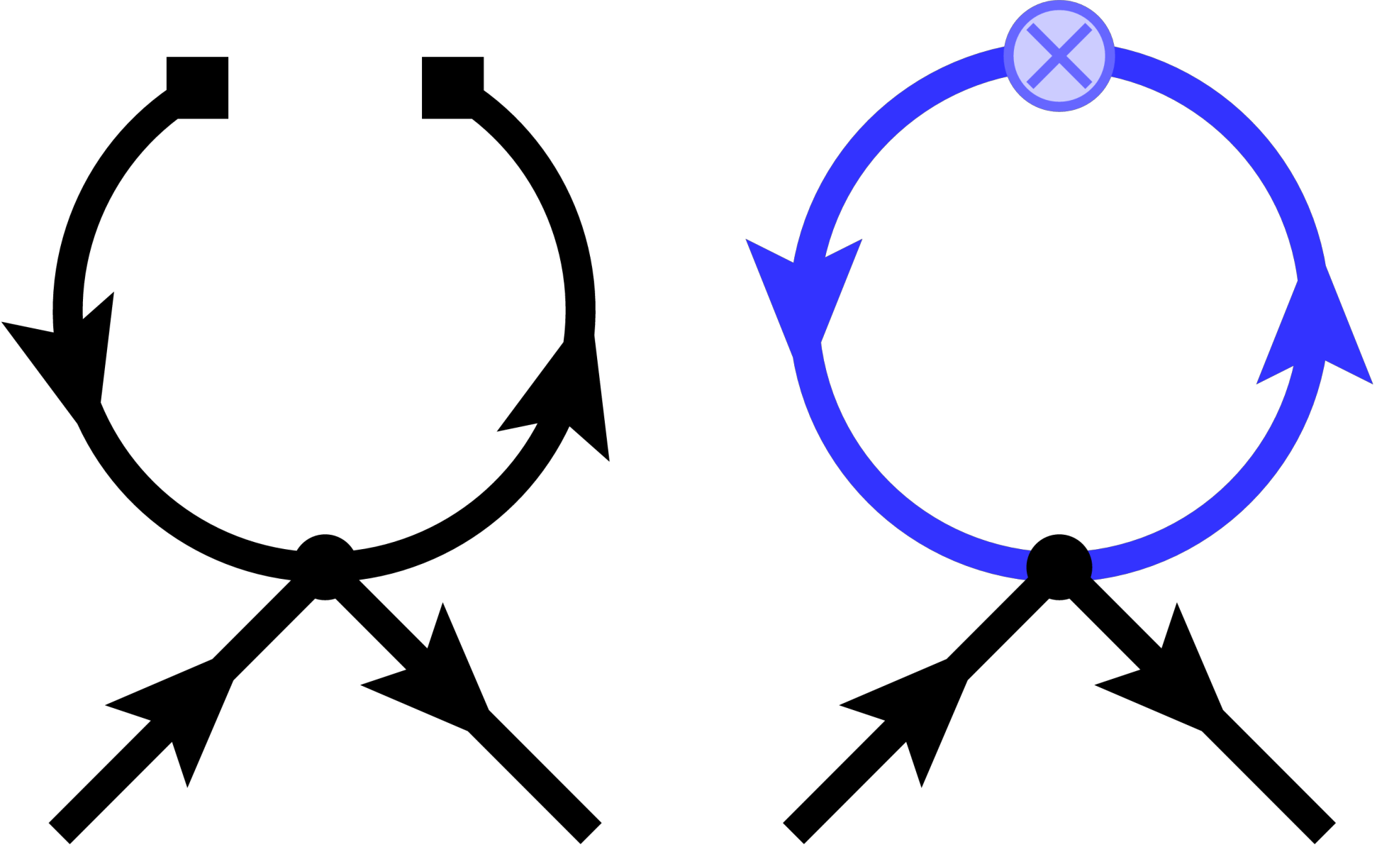

The smeared Wilson coefficient for the leading connected and disconnected operators are
| (10) | ||||
| (11) |
Here , and is the Euler-Mascheroni constant. The corresponding local Wilson coefficients in the scheme are
| (12) | ||||
| (13) |
Although we have expressed the smeared and local Wilson coefficients in different renormalisation schemes, so that we cannot directly compare the finite contributions, we note four features:
- 1.
The logarithmic dependence on the spacetime separation is the same.
- 2.
The flow time serves as the renormalisation scale for the leading order contributions.
- 3.
Wilson coefficients must be independent of the external states. We ensure this by choosing , or equivalently by taking the flow time sufficiently small that terms of can be neglected. This is easily seen by considering the derivative with respect to the external momenta of the integrand for [13]. Choosing the smearing radius smaller than the spacetime extent of the non-local operator ensures that the sOPE remains an (exponentially-)local expansion. In other words, if the gradient flow probes length scales on the order of the non-local operator, then the sOPE becomes a poor expansion for the original operator. This physical intuition underlies both the small flow-time expansion [11, 12] and the sOPE.
- 4.
The flow time cannot regularise the Wilson coefficients beyond the leading order contributions, because the flow evolution is classical and interactions necessarily appear at vanishing flow time (a higher-order calculation is given in [13]). However, the renormalisation scale dependence of the smeared operators is absorbed by the renormalisation parameters of the original theory.
4 Renormalisation group equations
The standard renormalisation group (RG) operator is
| (14) |
where
| (15) |
Here is the wavefunction renormalisation. In general the beta function, , and anomalous dimensions, and , are functions of the renormalised mass, , the renormalisation scale, , and the coupling constant, , and are known to five loops for an -symmetric theory [14].
For the sOPE, we must account for the extra flow time scale. If we choose , with a real number that ensures , then the smeared RG operator is . For small flow times, the smeared Wilson coefficient then obeys the smeared RG equation:
| (16) |
where is an anomalous dimension that parameterises the flow time dependence of the smeared operator [6, 12]. An analogous equation holds for the renormalised matrix elements of , which can be studied nonperturbatively.
Nonperturbative calculations:
We have so far considered the sOPE for in four spacetime dimensions, which is not asymptotically free. Therefore we briefly consider how the sOPE connects nonperturbative calculations to perturbative results for DIS calculations in QCD. The sOPE incorporates two scales, so a “line of constant physics” is a path for which the scales are tied together, for example, by fixing their product, .
Our aim is to connect hadronic matrix elements with smeared Wilson coefficients, which are determined in perturbation theory, at a suitably high scale using a finite-size scaling analysis [15]. We calculate matrix elements of smeared operators at some low energy scale, determined by the inverse box size, and take the continuum limit at fixed physical flow time. The smearing radius should be less than any hadronic scales present in the nonperturbative determination of the twist operators.
The scaling of the nonperturbative matrix elements is now entirely determined by the renormalisation scale dependence and we can apply a standard finite volume step-scaling procedure (see, for example, the step-scaling procedure for smeared operators in [16]) to some high scale. We choose the end point so that the new flow time is small relative to the experimentally determined inverse momentum transfer of the DIS process. At this new scale, the new renormalisation scale is sufficiently high that the nonperturbative matrix elements can be reliably combined with smeared Wilson coefficients.
5 Summary
We have proposed a new formalism, which we call the smeared operator product expansion (sOPE), to extract lattice matrix elements without power divergent mixing. The most obvious application is to deep inelastic scattering, but the sOPE can be applied to nonperturbative calculations that suffer from power-divergent mixing, such as the computations of decays and -meson mixing [17].
We expand non-local operators in a basis of smeared operators, generated via the gradient flow. The continuum limit of these matrix elements is free from power-divergent mixing, provided the smearing scale, or flow time, is kept fixed in the continuum limit. The matrix elements are then functions of both the renormalisation scale and the smearing length. The sOPE systematically relates these matrix elements to smeared Wilson coefficients, which are calculated perturbatively, and thus provides a complete framework in which to extract phenomenologically-relevant physics.
Acknowledgments.
We would like to thank Martin Lüscher and Andrea Shindler for enlightening and helpful discussions during the course of this work. This project was supported by the U.S. Department of Energy, Grant Number DE-FG02-04ER41302. K.O. was also supported by the U.S. Department of Energy through Grant Number DE-AC05-06OR23177, under which JSA operates the Thomas Jefferson National Accelerator Facility.References
- [1] P. Jimenez-Delgado, A. Accardi and W, Melnitchouk, Phys.Rev.D 89 (2014) 034025; R.D. Ball et al., Nucl.Phys.B 874 (2013) 36; F. Arbabifar, A.N. Khorramian and M. Soleymaninia, Phys.Rev.D 89 (2014) 034006; J.F. Owens and A. Accardi and W. Melnitchouk, Phys.Rev.D 87 (2013) 094012;
- [2] Y-Q. Ma and J-W. Qiu, (2014) [1404.6860]; X. Ji, Sci.China Phys.Mech.Astron. 57 (2014) 1407; X. Ji, Phys.Rev.Lett. 26 (2013) 110;
- [3] H. W. Lin et al., (2014) [1402.1462]
- [4] C. Monahan and K. Orginos, these proceedings
- [5] R. Narayanan and H. Neuberger, JHEP 0603 (2006) 064
- [6] M. Lüscher and P. Weisz, JHEP 1102 (2011) 051; M. Lüscher and P. Weisz, JHEP 1008 (2010) 071
- [7] M. Lüscher, JHEP 1304 (2013) 123;
- [8] C. Morningstar and M.J. Peardon, Phys.Rev.D 69 (2004) 054501;
- [9] Z. Davoudi and M.J. Savage, Phys.Rev.D 86 (2012) 054505
- [10] S. Hollands and C. Kopper, Commun.Math.Phys. 313 (2012) 257
- [11] A. Shindler, J. de Vries and T. Luu, (2014) [1409.2735]; A. Shindler, Nucl.Phys.B 881 (2014) 71; L. Del Debbio, A. Patella and A. Rago, JHEP 1311 (2013) 212; H. Suzuki, PTEP (2013) 083B03; H. Makino and H. Suzuki, PTEP (2014) 063B02; M. Asakawa et al., Phys.Rev.D 90 (2014) 011501
- [12] M. Lüscher, JHEP 1406 (2014) 105
- [13] C. Monahan and K. Orginos, in preparation
- [14] H. Kleinert and V. Schulte-Frohlinde, Critical properties of -theories, World Scientific 2001
- [15] M. Lüscher, P. Weisz and U. Wolff, Nucl.Phys.B 359 (1991) 221
- [16] C. Monahan and K. Orginos, \posPoS (Lattice2013) 443
- [17] C. Dawson et al., Nucl.Phys.B 514 (1998) 313-335; C. Monahan et al., Phys.Rev.D 90 (2014) 054015