Some cosmological models coming from gravitational theories having torsional degrees of freedom
Abstract
In this work we consider gravitational theories in which the effect of coupling characteristic classes, appropriately introduced as operators in the Einstein-Hilbert action, has been taken into account. As it is well known, this approach strays from the framework of general relativity since it results in theories in which torsion can be present. We consider here all the characteristic classes that are consistent with a four-dimensional space-time manifold. Then, we present explicit expressions for the contortion -form and torsion -form for a broad class of conditions in various cases of interest. Additionally, we use the same framework to study cosmological scenarios that are obtained mainly by selecting the flat FLRW metric and an ideal fluid.
Keywords:
torsion -form; contortion -form; ; general relativity; differential geometry; topological invariants; space-time topology1 INTRODUCTION
In recent years, the interest on gravitational theories with torsional degrees of freedom has steadily grown insomuch as they have exhibited interesting cosmological implications, as witnessed in the study of missing matter problems, as well as providing a new mechanism to explain the acceleration of the Universe based on modifications of general relativity (GR), instead of introducing an exotic content of matter.
It is well known that in the Einstein–Cartan theory the source of torsion is the spin current and hence the curvature and torsion become independent degrees of freedom of the gravitational field; however, in this theory, torsion has no dynamics and in four space-time dimensions it vanishes in the absence of sources. To overpass this, one can or add higher order corrections to the curvature or couple additional fields to gravity, resulting in theories with propagating torsion. Among the theories of gravity that encompass torsion, we can mention the Poincaré gauge theory of gravity, teleparallel gravity and -gravity, being the last two solely based on torsion. The introduction of torsion induces new physical effects and modifies the local degrees of freedom of the theory. For instance, the Einstein-Hilbert theory can be interpreted as a reduction of a higher dimensional model of the Chern-Simons type in which a propagating torsion solution naturally appears [1, 2]. The addition of torsion also enhances the possibility of an accelerated expansion of the universe among others scenarios [3, 4, 5, 6]. An authoritative review to the literature of space-time with torsion in cosmology is provided in [7]. Also, it has been proposed that the appearance of torsion would induce observable effects over the neutrino oscillation [8].
The theory considered here has no spin densities, but there is a propagating torsion due to the coupling of characteristic classes with scalar fields. We only consider characteristic classes consistent with a four-dimensional space-time manifold structure, i.e., those constructed from the rational cohomology ring, namely the Euler and the Pontryagin classes [9], as well as the Chern type Nieh-Yan class [10, 11] which is the only density immediately null in the absence of torsion, see also [12, 13]. The effects of adding the aforementioned classes can be acknowledged for by introducing a new term into the connection -form called contortion, which in turn is responsible for the torsion, see for instance [14].
An effective extension of GR by coupling the Pontryagin invariant with a (non-dynamical) scalar field in absence of torsion was studied in the literature on the so-called Chern-Simons gravity [15], whereas a generalization of this theory, in which the torsion was included, was considered in [16, 17] and the references therein, the theory being mainly motivated by anomaly cancellation in particle physics and string theory. In Ref. [18] four-dimensional gravity deformed by the Nieh-Yan invariant coupled to a scalar field was studied, and an exact solution to the theory was obtained, the so-called torsion vortex, which has an interesting holographic interpretation due to the correspondence. Furthermore, cosmological models of a theory where the Euler invariant was coupled to scalar field have been considered in [19], see also [20], the coupling of the scalar field to the Euler invariant can also arise from compactifications of a higher-dimensional theory of the Lovelock family [21]. On the other hand, slowly rotating black hole solutions to Chern-Simons gravity in the presence of torsion was presented in [22].
A somewhat similar approach to the one presented here has been used in [23, 24] were the focus was to study the effects of these couplings over the topology and differential structure of the associated symplectic manifold. This was driven by having in mind the later canonical quantization of the theory. Quantizing falls out of the scope of the present work and we refer the reader to [25, 26, 27] and the references therein for quantum aspects of theories with torsion.
This paper aims to consider gravitational theories beyond GR by allowing torsional degrees of freedom coming from all the characteristic classes known to be compatible with a four-dimensional space-time structure. These theories are first studied in a purely gravitational background setting, which results in obtaining analytical expressions for the important dynamical variables in the fashion of the first order formalism for all the cases considered. We then study several examples in a cosmological scenario, which may be capable to explain different stages of cosmic evolution without the need to introduce an exotic content of matter. The structure of the paper is as follows: in Section 2 we introduce some mathematical background required in the body of the work. In Section 3 we obtain explicit expressions for the torsion -form and the contortion -form for four different cases. In Section 4 we present the appropriate changes that must be carried out for the cosmological studies of these field equations. Consequently, we show several examples in which solutions have been obtained. Finally, we close with some remarks of the solutions shown on the body of the text.
2 GENERAL CONSIDERATIONS
We begin by summarizing the standard vierbein formalism and the basics of differential geometry needed in the next sections, see for instance [28, 29, 30, 31, 32]. On a four-dimensional space-time manifold with a cosmological constant , the Einstein-Hilbert action can be written as
| (1) |
where is the Newton constant, denotes the -form frame fields or vierbein and is a general connection -form, the latter defines the curvature to be
| (2) |
The Palatini variation of the action (1) gives the Einstein’s field equations and also, as an independent constraint, the null torsion condition
| (3) |
allowing to write the action as well as the connection entirely in terms of the vierbein (or ultimately in terms of the metric) as
| (4) |
where is the exterior derivative and is the interior or slant product with respect to the vierbein. We have also denoted . Eq. (4) defines the connection -form for GR, also known as the Levi-Civita connection. We can think of as being a -bundle or a -bundle space-time, depending on the signature of the metric.
For an oriented real four-manifold the characteristic classes available comprise the Stiefel-Whitney classes and the Euler and Pontryagin classes [9]. By allowing the four-manifold to be an almost complex smooth four-manifold the Chern classes can also be considered [9]. Among the previous possibilities we will specifically use the Pontryagin and Euler densities, as well as the Chern type Nieh-Yan density which has been proven to be important to study the spin structure of the theory in a quantum context [23, 24, 33, 34, 35]. These have, locally, the following representations as -forms, respectively.
| (5) | |||||
| (6) | |||||
| (7) | |||||
where we have denoted by a tilde the corresponding -form associated with each exact -form presented above in an obvious way.
From now on, we will denote the connection of GR (Levi-Civita connection) as , so that a generalized spin connection can split in the following form [18, 22, 36, 37, 38, 39, 40]
| (8) |
where is called the contortion. Therefore, the torsion 2-form can be written as
| (9) |
where is the covariant derivative with respect to the connection .
Hence, the contortion is the object responsible for the presence of torsion as anticipated. Similarly, using (2) and (8) the curvature -form can be written in the following way
| (10) |
where . Finally, the following, known as the Bianchi identities
| (11) | |||||
| (12) |
are satisfied.
2.1 The full action
It should be clear, following the discussion in the previous section, that knowing the Levi-Civita connection and the contortion -form is sufficient to describe all the physical observables of the theory. Hence, the problem narrows down to find an expression for . Let us address this by considering the following family of actions
| (13) |
where we have introduced the dimensionless fields , and the field with dimensions (collectively written as ) that serve as couples to the characteristic classes (5), (6) and (7) respectively. The coupling and are thought as being axionic fields whereas is a scalar field introduced in the family of actions (13) to generate torsion.
Note also that we can write the action (13) as
| (14) | |||||
where we used Stokes theorem to obtain the last term. Note that the action has several non-trivial contributions on the boundary that consequently give rise to several possibilities we need to analyze if we want to avoid extra complications when extremizing the action,
- 1.
is a parameter
Since the last term is an exact form it will not have contributions over the field equations. However, for a compact manifold with boundary there are non-linear higher derivative contributions coming from the characteristic densities acting over the boundary. If this is considered leads to nontrivial results in the context of AdS/CFT correspondence which are beyond the scope of the present work. The latter was studied in the following references [41, 42]. Also, in [43] it was shown that the Euler index appears in the Lagrangian for asymptotically locally AdS (ALADS) manifolds and in [44] it was shown the emergence of all three topological invariants for ALADS manifolds.
- 2.
is a map
Again, since the last term is an exact differential it will not have contributions on the field equations. However, this term will have nontrivial boundary conditions depending on the topology of the manifold considered. For instance, if is a compact manifold the maps are bounded with Neumann type of boundary conditions [45]. Since considering a boundary implies to adjust the boundary terms to behave like a generalized Gibbons-Hawking-York type of term [46], we will work with the particular case of closed manifolds (compact and without boundary) to avoid unnecessary discussion on the matter. Furthermore, this is consistent with the FLRW metric chosen to study cosmological scenarios in the subsequent sections.
3 EXPLICIT EXPRESSIONS FOR THE TORSION AND CONTORTION IN DIFFERENT TOPOLOGICAL SETUPS
Before tackling the problem described by the action introduced in section 2.1 (Eq. (14)), we propose few simplified cases in which we analyze the separated effect of the topological terms. We first take a look at the two simplest scenarios, where we consider the contributions from the Nieh-Yan and Pontryagin terms, and Pontryagin and Euler terms respectively; for these two cases in fact we can obtain explicit expressions. Consequently, we present two more cases that we approach in a more heuristic way. The latter cases describe the contribution of the Nieh-Yan and Euler terms and the last case in which all three terms are allowed to be present. As previously stated, we start by varying the action (14) considering to be maps, i.e. couplings as -forms and a compact manifold.
3.1 Case 1: Coupling Nieh-Yan and Pontryagin densities to the Einstein-Hilbert action
This first case can be carried out very straightforwardly. The field equations are
In order to solve this set of equations, we need to exclude the curvature and find an explicit expression for the contortion. This can be done by multiplying over Eq. (3.1). After, Eq. (3.1) can be used to obtain
| (23) |
where for an Euclidean metric with signature and for a Lorentzian metric with signature . For simplicity, we will consider the condition , thus, the above equation reduces to
| (24) |
and applying the interior product to this equation, we get
| (25) |
thus, the torsion is obtained straightforwardly to yield
| (26) |
where , are -forms that need to be adjusted in order to fulfill the rest of the restrictions imposed by the field equations. On the other hand, multiplying Eq. (3.1) by leads to
| (27) |
which in turn suggests the following expression for the curvature -form
where is an arbitrary function and , are 1-forms that must be determined from the remaining field equations. Additionally, by inserting Eqs. (26) and (3.1) in (3.1) yields . The contortion is obtained using (26) and (9)
| (28) |
which is manifestly skew-symmetric in the indices and . Note that by equations (26) and (28) we immediately recognize that . On the other hand, inserting Eq. (3.1) in Eq. (3.1), we find that the following expressions satisfy the resulting equation
| (29) |
where we have inserted , functions or -forms that must depend on the rest of the parameters and couplings only. However, notice that the expressions of the 1-forms and were not actually necessary for find the explicit expression for the torsion. Notice also, that , in contrast to , acquires an additional term due to the last term of Eq. (3.1). Then, taking into considerations restrictions (3.1) and (3.1) we obtain
| (30) |
The restrictions are not very illustrative for our purposes mainly because we need to use a definite metric and therefore its analysis will be postponed until section 4.
3.2 Case 2: Coupling Nieh-Yan and Euler characteristic invariants to the Einstein-Hilbert action
The second case we consider is also quite straightforward. By imposing in the action (14) the following field equations are obtained
with the last equation coinciding with Eq. (3.1), as expected. Here, the approach goes along the lines of what is presented in the previous subsection. Here we multiply to Eq. (3.2). After combining this result with Eq. (3.2), we get
| (39) |
In order to find an explicit expression for the torsion, we will consider , so, the above equation simplifies to
| (40) |
and the torsion is obtained straightforwardly to yield
| (41) |
where , are -forms which must be adjusted using the field equations. As in the previous section, when multiplying Eq. (3.2) by we obtain
| (42) |
which, in turn, suggests the following expression for the curvature -form
where is an arbitrary function and , are 1-forms that must be determined from the remaining field equations. Additionally, inserting Eqs. (41) and (3.2) in Eq. (3.2) yields
| (43) |
Finally, with the aid of Eq. (9) and Eq. (41) we find the contortion to be
| (44) |
which is manifestly skew-symmetric in the indices and . On the other hand, inserting Eq. (3.2) in Eq. (3.2), we find that the following expressions satisfy the resulting equation
| (45) |
where are arbitrary functions. Now, when taking into consideration the restrictions coming from Eqs. (3.2) and (3.2) we obtain
| (46) | |||||
respectively. As before, these restrictions are not very illustrative for our purposes mainly because we need to use a definite metric and therefore its analysis will be postponed until the section 4. However, notice that for the above constraints impose .
3.3 Case 3: Pontryagin and Euler characteristic invariants added to the Einstein-Hilbert action
Settting in (14) yields the following field equations
Note the presence of the field equations (3.3) and (3.3) which we have already encountered in the previous cases. The standard approach we used before cannot be applied here directly. In fact, combining Eqs. (3.3) and (3.3) will lead to expressions that cannot be cast in terms of the contortion and its interior products only. Hence, we take a more heuristic approach: taking the wedge product of and Eq. (3.3) and using (3.3) leads to
| (55) |
note that the curvature appears explicitly in the above equation. However, in the following, as we have been doing so far, we will consider , thus, Eq. (3.3) by itself suggests a curvature of the form
where
| (56) |
and where , , and are -forms that must depend on the rest of the parameters and couplings. Note that the exact expressions of the 1-forms and are not actually necessary to find an explicit expression for the torsion, as we will see. Now, by inserting Eq. (3.3) in Eq. (3.3) one obtains
| (57) |
and from the last expression the torsion is found to be
| (58) |
where , are arbitrary -form. These functions can be adjusted by inserting Eqs. (58) and (3.3) in (3.3), yielding
| (59) |
where we have denoted for an Euclidean like metric and for a Lorentzian like metric, as before. The contortion is found to be
| (60) |
On the other hand, inserting (3.3) into Eqs. (3.3) and (3.3) yields
| (61) | |||||
| (62) |
where, as before, we have assumed a condition of the type to simplify the aforementioned expressions. Starting from Eq. (61), when combined with Eq. (62), it is easy to obtain
| (63) |
for the auxiliary -form, which is valid only for Euclidean solutions, this is .
Inserting this expression back into Eq. (59) gives
| (64) |
which in turn, gives us the corresponding contortion
| (65) |
3.4 Case 4: Nieh-Yan, Pontryagin and Euler characteristic invariants added to the Einstein-Hilbert action
The more heuristic approach used on the previous case can also be applied here with some minor adjustments. Let us now consider the entire action (14), and its variation
As we have been assuming, for the sake of simplicity, we consider the couplings -forms to satisfy . When multiplying Eq. (3.4) by leads to
| (77) |
which in turn suggests the following expression for the curvature -form
where is an arbitrary function and , and are 1-forms that must be determined from the remaining field equations. However, as in the previous cases, it is possible to obtain an explicit expression for the torsion without knowing them. Analogously as in the previous cases, by multiplying Eq. (3.4) by combined with Eqs. () and (3.4), then, inserting this back in () yields the torsion
| (78) |
and the contortion reads
| (79) | |||||
Inserting Eq. (3.4) in Eq. (3.4), and based on the results of the previous sections, we get
| (80) |
where , and , and , are functions and . Then, taking into considerations restrictions (3.4), (3.4) and (3.4) we obtain
| (81) | |||||
| (82) | |||||
| (83) | |||||
respectively. So, from Eqs. (81), (82) and (83) we devise two possible solutions
- 1.
- 2.
In this case, similarly as in the previous case, we get
which is valid only for the Euclidean case, this is . The torsion and contortion read
(86) (87) respectively.
Note that in solutions (84) and (86), in the absence of a cosmological constant, the Nieh-Yan coupling can still generate torsional degrees of freedom by itself.
3.5 Matter source
We can add in the action (14) a term representing the matter source:
| (88) |
which, when varied with respect to the vierbein, yields the energy-momentum -form . Consequently, the term , where the represents the Hodge dual mapping, must be included in the left side of the field equation (3.4) or its equivalent in the other cases examined. Additionally, variation with respect to yields the spin current -form , thus, the term must be included in the left side of the field equation () or its equivalent in the other cases examined. It is known that the spin current is a source for torsion; however, this is not the only possibility. In the theory considered here, the gradient of the scalar fields , and are also source of torsion as we have shown in the above subsections; so, in our case we can have torsion even if the spin current is null. In the next section we will consider cosmological scenarios with a standard perfect fluid matter without spin .
3.6 Note
4 SOME COSMOLOGICAL SOLUTIONS
In this section we construct cosmological solutions having in mind the insights gained with the analytical expressions obtained on the previous section. We start then by choosing the following form for the metric
| (89) |
where for a Lorentzian metric, corresponding to the FLRW metric with flat spatial curvature, and for an Euclidean metric. We allow for the freedom in signature choice in order to recover interesting solutions that have been reported (for instance the torsion vortex metric [18]). The spacetime is assumed to be spatially flat, in accordance with the current observational evidence [47]. The vierbein is easily obtained to be
| (90) |
notice that this choice is not unique since many other veirbein give rise to the same metric. In fact, any local Lorentz transformation of the diagonal vierbein (90) give rise to the FLRW metric. However, note that in certain teleparallel theories, such as gravity, due to their lack of local Lorentz invariance, they become sensitive to the vierbein choice, for a recent review of these ideas see [48]. From (3) we obtain the following expressions for the Levi–Civita connection
| (91) |
where is the Hubble parameter, and denotes the time derivative of the scale factor .
A cosmological scenario is considered by adding in the action (14) a term representing the matter source (see subsection 3.5). In this work we will consider spinless matter, thus , and we model the dynamics by a simple pressure-less dust scenario described by a perfect fluid with energy-momentum -form , with density . Additionally, we argue that the couplings -forms are only dependent on the time coordinate, since, in order to describe realistic solutions, we need to encompass the observational properties of isotropy and homogeneity of our universe at large scales.
Eqs. (90) and (91) are then used to construct the corresponding contortion and torsion from the expressions founded in the previous section and the curvature from the Eq. (10) with labeling each of the cases considered in the previous section. We have to recall, though, that the expressions and we calculated have been obtained in the absence of matter and thus, must to be modified for the introduction of it. Consequently, having in mind Eq. (3.4) with a dust type of matter, it is easy to show that Eq. (77) behaves as follows: acquires the term and acquires the term for . Also, by using Eq. (), one finds that the expression obtained for the torsion is just Eq. (78) with the substitution .
Now, we take a look at the system of differential equations related to the case 4 since it is the one with all the couplings turned on. Using metric (89), from Eqs. (78) and (79) (with the substitution ) we obtain the expressions for the torsion and contortion, respectively. Then, from (10) we calculate the curvature -form. Finally, collecting all the field equations (3.4 - 3.4) we get the following system of equations
| (92) | |||||
| (93) | |||||
| (94) | |||||
| (95) | |||||
| (96) | |||||
| (97) | |||||
| (98) |
where we have set
| (99) | |||||
| (100) |
for convenience. Notice that Eqs. (96), (97) and (98) come from the variation with respect to the Euler, Pontryagin and Nieh-Yan terms respectively, and so are present in the case at hand while not being part of the set of equations when one or more of the characteristic classes are “switched off” from the start.
In fact, all the equations needed to describe the cases we considered in the previous section can be obtained from the system above, recalling that when we switched off one or more couplings, we did so at the level of the action. This leads to a change in the number of differential equations we then obtain from the action principle, beside of course the vanishing of the corresponding couplings in the remaining equations. We will also cover some cases not presented in section 3 but that can be obtained from these solutions and can have a cosmological interest.
4.1 Setting and
For this class of solutions we obtain , so either or . Having implies , i.e. we recover GR. If we consider , the torsion becomes null, and we recover the equations and solutions of GR, too
| (101) | |||||
| (102) |
However, the extra structure departing from GR shows itself in the presence of the Pontryagin and Nieh-Yan couplings that satisfy the following equation
| (103) |
Note also that if is constant then Eq. (103) implies that (with ) is a constant too, and vice versa. Since the solutions for the scale factor for GR are known, we are not considering them here.
4.2 Setting and
Although in principle this is not a case that was analyzed in section 3, it is clear from the equations obtained that the appearance of just one of the density classes is enough to have torsion. The set (92 - 97) thus allows us to study the present configuration which is interesting because of reproducing some models already found in literature. Note that in this case the system (92 - 97) looses the equations coming from the couplings and leading to
| (104) | |||||
| (105) |
where is an integration constant.
Additionally, the non-null components of the torsion tensor are given by
| (106) |
and using (105) we obtain that all of them are constants:
| (107) |
This torsion corresponds to the class, according to the classification of the torsion tensors given in [49] in terms of irreducible tensors in 4 dimensions.
It is worth to notice that considering combined with the energy-momentum conservation equation, which is contained in the above system of differential equations, we come to the conclusion that
| (108) |
which in principle represents a cosmological solution. We now present several sub-cases derived from the above
- 1.
for , and
(109) (110) (111) where is an integration constant. Note that Eq. (110) is exactly the solution known as the torsion vortex [18]. In fact, this solution corresponds to the one given in Eq. (33) of [18], with . Note also that in this paper and for an Euclidean metric (), corresponds to the anti-de Sitter case, because we have written the cosmological constant term in the action (1) with a plus sign. This choice was done in order that for a Lorentzian metric () with signature corresponds to the anti-de Sitter case.
- 2.
for , and , we obtain the following solution
(113) (114) with and integration constants. In Fig. 1 we show this set of solutions of , , and for , , and , where denotes the deceleration parameter, defined by
(115) It is interesting to note that the coupling zero-form is asymptotically slowly varying after . Consequently, the influence of torsion over the field equations becomes increasingly negligible for . Note also how the scale factor is non-decreasing, thus, suggesting a non-contracting universe. This is even clearer when examining Fig. 2, where we show the behavior of , and , all of them as a function of . We observe that the deceleration parameter is initially positive, then becomes negative and tends to a constant value, describing an accelerated expanding universe at later times.

Figure 1: Behavior of , , and for , , and 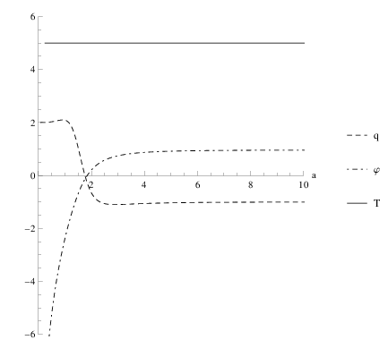
Figure 2: Behavior of , and as function of , for , , and
- 1.
for , and , the cosmological solutions coincide with those of equations (109 - 111), where we have plotted in Fig. 3 the set of solutions for , , and when , , , . We can see again how the coupling zero-form is asymptotically slowly varying after , hence, with negligible contribution in the field equations. This is better shown in Fig. 4 where the behavior of , and as a function of has been plotted. Notice the two branched, asymptotically slow varying solution for , as well as having a deceleration parameter that is initially negative, but that later increases monotonically to a constant negative value.

Figure 3: Behavior of , , and for , , and 
Figure 4: Behavior of , and as function of , for , , and - 2.
for , and we have
(116) In order to be physically admissible, at least as a model of the early stages of cosmic evolution, we must restrict the cosmic time to the interval , with . In this way is an increasing function of time. From equation (116), it is easily seen that the deceleration parameter yields
(118) - 3.
for , and we obtain
(119) (120)
This solution illustrates two monotonically increasing functions for and . It is straightforward from equation (119), it easily follows that
| (121) |
and hence, represents a decelerated expanding universe.
4.3 Setting and
As before, since only one coupling is needed to obtain torsion, we go to analyze the case in which only the Pontryagin class is present. When discarding equations coming from the Nieh-Yan invariant constraint and from the Euler invariant constraint, it can be shown that in the remaining system (92 - 97) not all equations are independent. Additionally, the non-null components of the torsion tensor are given by
tuning these into the and classes of torsion, according to the classification given in [49].
Several solutions are presented in what follows. First, for we recover the solutions of GR:
- 1.
for and
(123) (124) Representing a dark-energy dominated universe in standard cosmology.
- 2.
for
- (a)
(125) (126) yielding a deceleration parameter
(127) - (b)
(128) (129) yielding a deceleration parameter
(130) - (c)
(131) (132) which it is known to correspond to a matter dominated universe in standard cosmology.
- (a)
For and , from the system of equations one can obtain the following equations
| (133) |
| (134) |
and from this last equation we can only obtain an implicit solution for :
- 1.
(135) - 2.
(136) - 3.
(137)
It would be worth to study numerically the solutions obtained in this case and also study the case , .
4.4 Setting and
As before, this is a case that can be studied starting from the system (92 - 97). This was not a case considered in section 3, however, it shows some interesting features. When discarding those equations coming from Nieh-Yan invariant constraint and from the Pontryagin invariant constraint, the remaining system contains the conservation Eq. (108). In this case, the non-null components of the torsion tensor are given by
that can be classified as and classes of torsion, according to [49].
After solving the remaining system the following admissible solutions are derived
- 1.
for and
(139) (140) (141) In Fig. 5 we show this set of solutions of , , , and for , and . Note that becomes imaginary for , this makes the solution valid only for .We see that the scale factor increases monotonically after , suggesting an expanding universe at later times. We also see that the coupling zero-form is decreasing monotonically. This can be further seen in Fig. 6, where we show the behavior of , and as a function of . Note the two branching solution of the coupling zero-form and how the deceleration parameter stabilizes in a constant negative number, meaning that the universe described by this model is an expanding universe.

Figure 5: Behavior of , , , and for , and 
Figure 6: Behavior of , , and as function of , for , and - 2.
for and
(142) (143) (144) In this case increases linearly with time. Notice that an Euclidean metric with only satisfies the condition .
5 FINAL REMARKS
In this work, we studied gravitational theories with propagating torsion, which arises by adding to the Einstein-Hilbert action combinations of the characteristic densities of a space-time manifold coupled with scalar fields. We have found explicit expressions for the contortion -form, given by Eqs. (28), (44), (60) and (79), consequently, expressions for the torsion (26), (41), (59) and (78) for a broad class of situations. These expressions were obtained in terms of the vierbein, the scalar fields (couplings) and their derivatives, only. One interesting feature of such analytical expressions is that important terms depend linearly on the cosmological constant, hence, since observation suggests the existence and positivity of this term, it is tempting to theorize that torsional degrees of freedom could be eventually measured. On the other hand, the strict dependency on the scalar fields shows that torsion becomes null when the couplings are null or constants, recovering the solution of Einstein-Cartan gravity as expected.
Since the cases of section 3 were studied in a coordinate free fashion, another alternative to encompass the task of study the material presented here is to consider a different metric than the one used here. This program will allow to find some known solutions as well as possibly new ones and will be considered in future works.
On the other hand, by taking a metric such as the one showed in (89), compatible with the topological assumptions that a space-time is a closed manifold, we were able to reproduce some well known models in a more or less general framework, for instance the torsion vortex solution reported in [18]. Furthermore, we obtained analytically new classes of cosmological solutions for the analyzed cases. These solutions describe physically relevant space-times representing different stages of cosmic evolution. Much more work is certainly necessary to fully study cosmological solutions and it will be tackled in subsequent papers, as well as considering the presence of different kinds of matter fields. Probably, by doing so, the analyticity of the solutions will be lost for which the use of numerical techniques is to be expected.
6 Acknowledgements
The authors want to thank Gastón Giribet for his comments and valuable suggestions for starting this work. The authors also want to thank Michele Fontanini for his valuable corrections, comments and suggestions in the final steps of this work. This work was funded by the Comisión Nacional de Ciencias y Tecnología through FONDECYT Grant 11121148 (Y.V., J.L.). J.L. acknowledge the hospitality of the Universidad de La Serena where part of this work was carried out.
References
- [1] B. Zumino, Gravity Theories in More Than Four-Dimensions, Phys.Rept. 137 (1986) 109. doi:10.1016/0370-1573(86)90076-1.
- [2] M. Banados, L. J. Garay, M. Henneaux, The Dynamical structure of higher dimensional Chern-Simons theory, Nucl.Phys. B476 (1996) 611–635. arXiv:hep-th/9605159, doi:10.1016/0550-3213(96)00384-7.
- [3] I. Buchbinder, S. Odintsov, I. Shapiro, NONSINGULAR COSMOLOGICAL MODEL WITH TORSION INDUCED BY VACUUM QUANTUM EFFECTS, Phys.Lett. B162 (1985) 92–96. doi:10.1016/0370-2693(85)91067-6.
- [4] N. J. Poplawski, Cosmology with torsion - an alternative to cosmic inflation, Phys.Lett. B694 (2010) 181–185. arXiv:1007.0587, doi:10.1016/j.physletb.2010.09.056,10.1016/j.physletb.2011.05.047.
- [5] S. Capozziello, R. Cianci, C. Stornaiolo, S. Vignolo, f(R) cosmology with torsion, Phys.Scripta 78 (2008) 065010. arXiv:0810.2549, doi:10.1088/0031-8949/78/06/065010.
- [6] C. G. Boehmer, J. Burnett, Dark spinors with torsion in cosmology, Phys.Rev. D78 (2008) 104001. arXiv:0809.0469, doi:10.1103/PhysRevD.78.104001.
- [7] D. Puetzfeld, New Astron. Rev. 49, 59 (2005) [gr-qc/0404119].
- [8] M. Adak, T. Dereli, L. Ryder, Neutrino oscillations induced by space-time torsion, Class.Quant.Grav. 18 (2001) 1503–1512. arXiv:gr-qc/0103046, doi:10.1088/0264-9381/18/8/307.
- [9]
S. Donaldson, P. Kronheimer,
The Geometry of
Four-manifolds, Oxford mathematical monographs, Clarendon Press, 1990.
URL http://books.google.com.br/books?id=RWPpngEACAAJ - [10] H. T. Nieh and M. L. Yan, “An Identity in Riemann-cartan Geometry,” J. Math. Phys. 23, 373 (1982).
- [11] H. T. Nieh and C. N. Yang, “A torsional topological invariant,” Int. J. Mod. Phys. A 22, 5237 (2007).
- [12] S. Li, The Topological structure of Nieh-Yan form and chiral anomaly in spaces with torsion, J.Phys. A32 (1999) 7153–7162. arXiv:hep-th/9905058, doi:10.1088/0305-4470/32/41/309.
- [13] G. Date, R. K. Kaul and S. Sengupta, “Topological Interpretation of Barbero-Immirzi Parameter,” Phys. Rev. D 79, 044008 (2009) [arXiv:0811.4496 [gr-qc]].
- [14] P. Baekler, F. W. Hehl, Beyond Einstein-Cartan gravity: Quadratic torsion and curvature invariants with even and odd parity including all boundary terms, Class.Quant.Grav. 28 (2011) 215017. arXiv:1105.3504, doi:10.1088/0264-9381/28/21/215017.
- [15] R. Jackiw and S. Y. Pi, “Chern-Simons modification of general relativity,” Phys. Rev. D 68, 104012 (2003) [gr-qc/0308071].
- [16] M. B. Cantcheff, “Einstein-Cartan formulation of Chern-Simons Lorentz Violating Gravity and Holographic Structure,” Phys. Rev. D 78, 025002 (2008) [arXiv:0801.0067 [hep-th]].
- [17] S. Alexander and N. Yunes, “Chern-Simons Modified General Relativity,” Phys. Rept. 480, 1 (2009) [arXiv:0907.2562 [hep-th]].
- [18] R. G. Leigh, N. N. Hoang, A. C. Petkou, Torsion and the Gravity Dual of Parity Symmetry Breaking in AdS(4) / CFT(3) Holography, JHEP 0903 (2009) 033. arXiv:0809.5258, doi:10.1088/1126-6708/2009/03/033.
- [19] A. Toloza, J. Zanelli, Reflections on Cosmology: an Outsider’s Point of View, AIP Conf.Proc. 1471 (2012) 16–21. arXiv:1204.1380, doi:10.1063/1.4756805.
- [20] A. Toloza, J. Zanelli, Cosmology with scalarâEuler form coupling, Class.Quant.Grav. 30 (2013) 135003. arXiv:1301.0821, doi:10.1088/0264-9381/30/13/135003.
- [21] A. Mardones and J. Zanelli, “Lovelock-Cartan theory of gravity,” Class. Quant. Grav. 8, 1545 (1991).
- [22] M. Cambiaso, L. F. Urrutia, An extended solution space for Chern-Simons gravity: the slowly rotating Kerr black hole, Phys.Rev. D82 (2010) 101502. arXiv:1010.4526, doi:10.1103/PhysRevD.82.101502.
- [23] R. K. Kaul, S. Sengupta, Topological parameters in gravity, Phys.Rev. D85 (2012) 024026. arXiv:1106.3027, doi:10.1103/PhysRevD.85.024026.
- [24] S. Sengupta, SU(2) gauge theory of gravity with topological invariants, J.Phys.Conf.Ser. 360 (2012) 012024. arXiv:1110.4185, doi:10.1088/1742-6596/360/1/012024.
- [25] I. L. Shapiro, “Physical aspects of the space-time torsion,” Phys. Rept. 357, 113 (2002) [hep-th/0103093].
- [26] R. K. Kaul and S. Sengupta, “Torsional instanton effects in quantum gravity,” Phys. Rev. D 90, no. 12, 124081 (2014) [arXiv:1411.4793 [gr-qc]].
- [27] S. Sengupta, “A quantum gravitational origin of dark energy,” arXiv:1501.00779 [gr-qc].
- [28] P. Dona, S. Speziale, Introductory lectures to loop quantum gravityarXiv:1007.0402.
- [29] D. Giulini, Ashtekar variables in classical general relativityarXiv:gr-qc/9312032.
- [30]
M. Nakahara, Geometry,
Topology and Physics, Second Edition, Graduate student series in physics,
Taylor & Francis, 2003.
URL http://books.google.be/books?id=cH-XQB0Ex5wC - [31]
C. Nash, S. Sen, Topology
and geometry for physicists, Academic Press, 1983.
URL http://books.google.cl/books?id=Lz7y9PmTdgwC - [32]
A. Hatcher, Algebraic
Topology, Cambridge University Press, 2002.
URL http://books.google.cl/books?id=BjKs86kosqgC - [33] S. Mercuri and A. Randono, “The Immirzi Parameter as an Instanton Angle,” Class. Quant. Grav. 28, 025001 (2011) [arXiv:1005.1291 [hep-th]].
- [34] S. Sengupta, “Quantum realizations of Hilbert-Palatini second-class constraints,” Class. Quant. Grav. 27, 145008 (2010) [arXiv:0911.0593 [gr-qc]].
- [35] T. Liko, Barbero-Immirzi parameter, manifold invariants and Euclidean path integrals, Class.Quant.Grav. 29 (2012) 095009. arXiv:1111.6702, doi:10.1088/0264-9381/29/9/095009.
- [36] Y. Cho, B. Park, D. Pak, A Minimal model of Lorentz gauge gravity with dynamical torsion, Int.J.Mod.Phys. A25 (2010) 2867–2882. arXiv:0911.3688, doi:10.1142/S0217751X10048524.
- [37] A. Hatzinikitas, Locally Weyl invariant massless bosonic and fermionic spin 1/2 action in the (W(n)(4),g) and (U(4),g) space-times, Gen.Rel.Grav. 32 (2000) 2287–2294. arXiv:gr-qc/9911059, doi:10.1023/A:1001999525571.
- [38] A. C. Petkou, Torsional degrees of freedom in AdS4/CFT3arXiv:1004.1640.
- [39] O. Chandia, J. Zanelli, Topological invariants, instantons and chiral anomaly on spaces with torsion, Phys.Rev. D55 (1997) 7580–7585. arXiv:hep-th/9702025, doi:10.1103/PhysRevD.55.7580.
- [40] O. Randal-Williams, Relations among tautological classes revisited, ArXiv e-printsarXiv:1012.1430.
- [41] R. Aros, M. Contreras, R. Olea, R. Troncoso, J. Zanelli, Conserved charges for gravity with locally AdS asymptotics, Phys.Rev.Lett. 84 (2000) 1647–1650. arXiv:gr-qc/9909015, doi:10.1103/PhysRevLett.84.1647.
- [42] O. Miskovic, R. Olea, Topological regularization and self-duality in four-dimensional anti-de Sitter gravity, Phys.Rev. D79 (2009) 124020. arXiv:0902.2082, doi:10.1103/PhysRevD.79.124020.
- [43] R. Aros, M. Contreras, R. Olea, R. Troncoso and J. Zanelli, “Conserved charges for even dimensional asymptotically AdS gravity theories,” Phys. Rev. D 62, 044002 (2000) [hep-th/9912045].
- [44] S. Sengupta, “Gravity Asymptotics with Topological Parameters,” Phys. Rev. D 88, no. 2, 024031 (2013) [arXiv:1304.7597 [gr-qc]].
- [45] Lambert, B. 2014, arXiv:1408.5309
- [46] E. Dyer and K. Hinterbichler, Phys. Rev. D 79, 024028 (2009) [arXiv:0809.4033 [gr-qc]].
- [47] E. Komatsu et al. [WMAP Collaboration], Astrophys. J. Suppl. 192, 18 (2011) doi:10.1088/0067-0049/192/2/18 [arXiv:1001.4538 [astro-ph.CO]].
- [48] Y. F. Cai, S. Capozziello, M. De Laurentis and E. N. Saridakis, arXiv:1511.07586 [gr-qc].
- [49] S. Capozziello, G. Lambiase and C. Stornaiolo, Annalen Phys. 10, 713 (2001) doi:10.1002/1521-3889(200108)10:8<713::AID-ANDP713>3.0.CO, 10.1002/1521-3889(200108)10:8<713::AID-ANDP713>3.0.CO;2-2 [gr-qc/0101038].