Secure and Green SWIPT in Distributed Antenna Networks with Limited Backhaul Capacity
Abstract
This paper studies the resource allocation algorithm design for secure information and renewable green energy transfer to mobile receivers in distributed antenna communication systems. In particular, distributed remote radio heads (RRHs/antennas) are connected to a central processor (CP) via capacity-limited backhaul links to facilitate joint transmission. The RRHs and the CP are equipped with renewable energy harvesters and share their energies via a lossy micropower grid for improving the efficiency in conveying information and green energy to mobile receivers via radio frequency (RF) signals. The considered resource allocation algorithm design is formulated as a mixed non-convex and combinatorial optimization problem taking into account the limited backhaul capacity and the quality of service requirements for simultaneous wireless information and power transfer (SWIPT). We aim at minimizing the total network transmit power when only imperfect channel state information of the wireless energy harvesting receivers, which have to be powered by the wireless network, is available at the CP. In light of the intractability of the problem, we reformulate it as an optimization problem with binary selection, which facilitates the design of an iterative resource allocation algorithm to solve the problem optimally using the generalized Bender’s decomposition (GBD). Furthermore, a suboptimal algorithm is proposed to strike a balance between computational complexity and system performance. Simulation results illustrate that the proposed GBD based algorithm obtains the global optimal solution and the suboptimal algorithm achieves a close-to-optimal performance. Besides, the distributed antenna network for SWIPT with renewable energy sharing is shown to require a lower transmit power compared to a traditional system with multiple co-located antennas.
Index Terms:
Limited backhaul, physical layer security, wireless information and power transfer, distributed antennas, green energy sharing, non-convex optimization.I Introduction
Next generation wireless communication systems are required to provide high speed, high security, and ubiquitous communication with guaranteed quality of service (QoS). These requirements have led to a tremendous energy consumption in both transmitters and receivers. Multiple-input multiple-output (MIMO) technology has emerged as a viable solution for reducing the system power consumption. In particular, multiuser MIMO, where a transmitter equipped with multiple antennas serves multiple single-antenna receivers, is considered to be an effective solution for realizing the performance gain offered by multiple antennas. On the other hand, energy harvesting based mobile communication system design facilitates self-sustainability for energy limited communication networks. For instance, the integration of energy harvesting devices into base stations for scavenging energy from traditional renewable energy sources such as solar and wind has been proposed for providing green communication services [3]–[5]. However, theses natural energy sources are usually location and climate dependent and may not be suitable for portable mobile receivers.
Recently, wireless power transfer has been proposed as an emerging alternative energy source, where the receivers scavenge energy from the ambient radio frequency (RF) signals [6]–[17]. The broadcast nature of wireless channels facilitates one-to-many wireless charging, which eliminates the need for power cords and manual recharging, and enables the possibility of simultaneous wireless information and power transfer (SWIPT). The introduction of an RF energy harvesting capability at the receivers leads to many interesting and challenging new research problems which have to be solved to bridge the gap between theory and practice. In [9] and [10], the fundamental trade-off between harvested energy and wireless channel capacity was studied for point-to-point and multiple-antenna wireless broadcast systems, respectively. In [11], it was shown that RF energy harvesting can improve the energy efficiency of communication networks. In [12], the authors solved the energy efficiency maximization problem for large scale multiple-antenna SWIPT systems. In [13], the optimal energy transfer dowlink duration was optimized to maximize the uplink average information transmission rate. The combination of physical (PHY) layer security and SWIPT was recently investigated in [14]–[17] for total transmit power minimization, secrecy rate maximization, max-min fair optimization, and multi-objective optimization, respectively. Nevertheless, despite the promising results in the literature [9]–[17], the performance of wireless power/energy transfer systems is still severely limited by the distance between the transmitter(s) and the receiver(s) due to the high signal attenuation caused by path loss and shadowing, especially in outdoor environments. Thus, an exceedingly large transmit power is required to provide QoS in information and power transfer. Hence, the energy consumption at the transmitters of wireless power transfer systems will become a financial burden to service providers if the efficiency of wireless power transfer cannot be improved and the energy cost at the transmitters cannot be reduced.
In this context, distributed antennas are an attractive technique for reducing network power consumption and extending service coverage [18]–[22]. A promising option for the system architecture of distributed antenna networks is the splitting of the functionalities of the base station between a central processor (CP) and a set of low-cost remote radio heads (RRHs). In particular, the CP performs the power hungry and computationally intensive baseband signal processing while the RRHs are responsible for all RF operations such as analog filtering and power amplification. The RRHs are distributed across the network and connected to the CP via backhaul links. This system architecture is known as “Cloud Radio Access Network” (C-RAN) [23, 24, 25]. The distributed antenna system architecture reduces the distance between transmitters and receivers. Furthermore, it inherently provides spatial diversity for combating path loss and shadowing. It has been shown in [18, 19] that distributed antenna systems with full cooperation between the transmitters achieve a superior performance compared to co-located antenna systems. Yet, transferring the information data of all users from the CP to all RRHs, as is required for full cooperation, may be infeasible when the capacity of the backhaul links is limited. Hence, resource allocation for distributed antenna networks with finite backhaul capacity has attracted considerable attention in the research community [20]–[22]. In [20], the authors studied the energy efficiency of distributed antenna multicell networks with capacity constrained backhaul links. In [21] and [22], iterative algorithms were proposed to reduce the total system backhaul capacity consumption while guaranteeing reliable communication to the mobile users. However, the problem formulations in [21] and [22] do not constrain the capacity consumption of individual backhaul links which may lead to an information overflow in some of the backhaul links. Moreover, [20]–[22] assume the availability of an ideal power supply for each RRH such that a large amount of energy can be continuously used for operation of the system whenever needed. However, assuming availability of an ideal power supply for the RRHs may not be realistic in practice, especially in developing countries or remote areas [20]–[22]. In addition, the receivers in [18]–[22] were assumed to be powered by constant energy sources which may also not be a valid assumption for energy-limited handheld devices. Although the transmitters can be powered by renewable green energy and the signals transmitted in the RF by the RRHs could be exploited as energy sources to the receivers for extending their lifetimes, resource allocation algorithm design for utilizing green energy in distributed antenna SWIPT systems has not been considered in the literature, yet.
Motivated by the aforementioned observations, in this paper, we propose the use of distributed antenna communication networks for transferring information and green renewable energy to mobile receivers wirelessly. We formulate the resource allocation algorithm design as a non-convex optimization problem. Taking into account the limited backhaul capacity, the harvested renewable energy sharing between RRHs, and the imperfect CSI of the energy harvesting receivers, we minimize the total network transmit power while ensuring the QoS of the wireless receivers for both secure communication and efficient wireless power transfer. To this end, we propose an optimal iterative algorithm based on the generalized Bender’s decomposition. In addition, we propose a low complexity suboptimal resource allocation scheme based on the difference of convex functions (d.c.) programming which provides a locally optimal solution for the considered optimization problem.
II System Model
II-A Notation
We use boldface capital and lower case letters to denote matrices and vectors, respectively. , , and represent the Hermitian transpose, the trace, and the rank of matrix , respectively; and indicate that is a positive definite and a positive semidefinite matrix, respectively; denotes the vectorization of matrix by stacking its columns from left to right to form a column vector. is the identity matrix; and denote the set of all matrices with complex and real entries, respectively; denotes the set of all Hermitian matrices; denotes a diagonal matrix with the diagonal elements given by ; and denote the absolute value of a complex scalar and the -norm of a vector, respectively. In particular, is known as the -norm of a vector and denotes the number of non-zero entries in the vector; the circularly symmetric complex Gaussian (CSCG) distribution is denoted by with mean and variance ; stands for “distributed as”; ; denotes a column vector with all elements equal to one. returns the -th element of the input matrix, is the -th unit column vector, i.e., and ; and for a real valued continuous function , represents the gradient of with respect to vector .

II-B Distributed Antenna System Model and Central Processor
We consider a distributed antenna multiuser downlink communication network. The system consists of a CP, RRHs, information receivers (IRs), and energy harvesting receivers (ERs), cf. Figure 1. Each RRH is equipped with transmit antennas. The IRs and ERs are single antenna devices which exploit the received signal powers in the RF for information decoding and energy harvesting, respectively. In practice, the ERs may be idle IRs which are scavenging energy from the RF to extend their lifetimes. On the other hand, the CP is the core unit of the network, which has the data intended for all IRs. Besides, we assume that all computations are performed in the CP. In particular, based on the available CSI, the CP computes the resource allocation policy and broadcasts it to all RRHs. Each RRH receives the control signals for resource allocation and the data of the IRs from the CP via a backhaul link. The backhaul links can be implemented with different last-mile communication technologies such as digital subscriber line (DSL) or out-of-band microwave links. Thus, the backhaul capacity may be limited. Furthermore, we assume that the CP is integrated with a constant energy source (e.g., a diesel generator) for supporting its normal operation, and the distributed RRHs are equipped with traditional energy harvesters such as solar panels and wind turbines for generation of renewable energy. The harvested energy can be exchanged between the CP and the RRHs over a micropower grid and the CP manages the energy flow in the micropower grid11 1 The proposed system can be viewed as a hybrid information and energy distribution network. In particular, the green energy harvested at the RRHs is shared via the micro-grid and distributed to the ERs via RF. , cf. Section II-F.
II-C Channel Model
We focus on a frequency flat fading channel and a time division duplexing (TDD) system. The wireless information and power transfer from the RRHs to the receivers is divided into time slots. The received signals at IR and ER in one time slot are given by
| (1) |
respectively, where denotes the joint transmit vector of the RRHs to the IRs and the ERs. The channel between the RRHs and IR is denoted by , and we use to denote the channel between the RRHs and ER . We note that the channel vector captures the joint effects of multipath fading and path loss. and include the joint effects of thermal noise, signal processing noise, and possibly present received multicell interference at IR and ER , respectively, and are modeled as additive white Gaussian noise (AWGN) with zero mean and variances and , respectively.
II-D Channel State Information
We assume that , and , can be reliably obtained at the beginning of each scheduling slot by exploiting the channel reciprocity and the pilot sequences in the handshaking signals exchanged between the RRHs and the receivers. Besides, the estimate of is refined at the CP during the entire scheduling slot based on the pilot sequences contained in acknowledgement packets. As a result, we can assume that the CSI for the RRHs-to-desired IR links is perfect during the entire transmission period. In contrast, the ERs do not interact with the RRHs during information transmission. Thus, the CSI of the ERs may be outdated during transmission and we use a deterministic model [14, 26] for characterizing the resulting CSI uncertainty. More precisely, the CSI of the link between the RRHs and ER is given by
| (2) |
where is the channel estimate of ER available at the CP at the beginning of a scheduling slot. represents the unknown channel uncertainty of ER due to the slowly time varying nature of the channel during transmission. In (2), we define set which contains all possible CSI uncertainties of ER . Specifically, specifies an ellipsoidal uncertainty region for the estimated CSI of ER , where and represent the radius and the orientation of the region, respectively. For instance, (2) represents an Euclidean sphere when . In practice, the value of depends on the coherence time of the associated channel and depends on the adopted channel estimation method.

II-E Signal and Backhaul Models
In each scheduling time slot, independent signal streams are transmitted simultaneously to the IRs. Specifically, a dedicated beamforming vector, , is allocated to IR at RRH to facilitate information transmission. For the sake of presentation, we define a super-vector for IR as
| (3) |
Here, represents the joint beamformer used by the RRHs for serving IR . Then, the information signal to IR , , can be expressed as
| (4) |
where is the data symbol for IR and , is assumed without loss of generality. The information signals intended for the desired IRs can be overheard by the ERs that are in the range of service coverage. Since the ERs may be malicious, they may eavesdrop the information signal of the selected IRs. This has to be taken into account for resource allocation design for providing secure communication services in the considered distributed antenna network. Thus, to guarantee communication security, the RRHs have to employ a resource allocation algorithm that accounts for this unfavourable scenario and treat the ERs as potential eavesdroppers22 2 Although the ERs are low-power devices, malicious ERs do not have to decode the eavesdropped information in real time. They can act as information collectors which sample the received signals and store them for future decoding by other energy unlimited and computationally powerful devices., see also [14, 15, 27, 28]. To this end, artificial noise is transmitted by the RRHs33 3 In [29], the secrecy rate achievable with regularized channel inversion for large numbers of users and transmit antennas was studied. However, the method proposed in [29] can guarantee a strictly positive secrecy rate only if the number of transmit antennas tends to infinity. which can be used to degrade the channels between the RRHs and the potential eavesdroppers and to serve as an energy source for the ERs. Hence, the transmit signal vector at the RRHs is given by
| (5) |
where is the artificial noise vector generated by the RRHs and modeled as a complex Gaussian random vector, i.e., , where , denotes the covariance matrix of . The artificial noise interferes the IRs and ERs since is unknown to both types of receivers. Hence, artificial noise transmission has to be carefully designed to degrade the channels of the ERs while having a minimal effect on the IRs. In fact, the covariance matrix of the artificial noise will be optimized under the proposed optimization framework. We note that artificial noise vector can be generated locally at the RRHs and does not have to be sent via the backhaul links. On the other hand, the data of each IR is delivered from the CP to the RRHs via backhaul links. The backhaul capacity consumption for backhaul link is given by
| (6) |
where is the required backhaul data rate for conveying the data of IR to a RRH and counts the number of IRs consuming the capacity of backhaul . We note that the backhaul links may be capacity-constrained and the CP may not be able to send the data of all IRs to all RRHs as required for full cooperation. Thus, to reduce the load on the backhaul links, the CP can enable partial cooperation by sending the data of IR only to a subset of the RRHs. In particular, by setting , RRH is not participating in the joint data transmission to IR . Thus, the CP is not required to send the data for IR to RRH via the backhaul link which leads to a lower information flow in the backhaul link.
II-F RRH Power Supply Model
The constant energy source of the CP transfers energy to all RRHs via a dedicated power grid (micropower grid) for supporting the power consumption at the RRHs and facilitating a more efficient network operation, cf. Figure 2. In particular, a bus in Figure 2 refers to the internal power line connection of zero impedance between two elements. The CP is connected to a point of common coupling to convey energy to the micropower grid and has full control over the micropower grid.
Since each RRH is equipped with energy harvesters for harvesting renewable energy, the energy harvested by the RRHs can also be shared in the communication system via the micropower grid. By exploiting the spatial diversity inherent to the distributed antenna network also for energy harvesting, we can overcome potential energy harvesting imbalances in the network for improving the system performance. In other words, there are energy sources for supporting the CP and the RRHs. We denote the unit of energy transferred from energy source to the micro-grid as where the power generator at the CP is the -th energy source. The power loss in delivering the power from all the energy sources to the RRH is given by [30]
| (7) |
where , . is known as the B-coefficient and , , is the B-coefficient matrix [30] which takes into account the distance dependent power line resistance, the phase angles of the electrical currents, and the voltages generated by the different energy sources. We note that the B-coefficient matrix is a constant for a fixed number of loads and a fixed grid connection topology. We assume that the B-coefficient matrix is known to the CP for energy allocation from long term measurements. Furthermore, the energy supplied by energy source is given by
| (8) |
where is the maximum energy available at energy source and represents the total amount of energy generated by energy source . In this paper, each energy source is able to adjust the amount of energy injected into the micropower grid.
In practice, the coherence time of the communication channel is much shorter than that of the renewable energy harvesting process at the RRHs. For instance, for a carrier center frequency of MHz and m/s receiver speed, the coherence time for wireless communication is in the order of ms. In other words, the resource allocation policy has to be updated roughly every ms. On the other hand, the renewable energy arrival rate at the energy harvesters of the RRHs changes relatively slowly. For example, solar energy and wind energy change in the order of a few tens of seconds [5]. Thus, for resource allocation design, we assume that in (8) is a known constant. Furthermore, we focus on the resource allocation for small cell systems, i.e., the inter-site distances between the RRHs is in the order of hundreds of meters. Thus, the energy propagation delay between two renewable energy harvesters is less than s, which is negligibly small compared to the coherence time of the communication channel and can be neglected in the power supply model.
III Problem Formulation
In this section, we define the QoS metrics for the design of secure communication and power efficient wireless energy transfer. Then, the resource allocation algorithm design is formulated as a non-convex optimization problem.
III-A Achievable Data Rate and RF Energy Harvesting
The achievable data rate (bit/s/Hz) between the RRHs and IR is given by
| (9) | |||||
| (10) |
is the receive signal-to-interference-plus-noise ratio (SINR) at IR .
Since the computational capability of the ERs (potential eavesdroppers) is not known at the CP, we consider the worst-case scenario for providing communication security. Specifically, in the worst case, the ERs are able to remove all multiuser interference and multicell interference via successive interference cancellation before attempting to decode the information of desired IR . Therefore, the achievable data rate between the RRHs and ER (potential eavesdropper) is given by
| (11) | |||||
| (12) | |||||
where is the received SINR at ER and is the joint power of the signal processing noise and the thermal noise. reflects the aforementioned worst-case assumption44 4 We note that the proposed framework can be easily extended to the case when a single-user detector is employed at the potential eavesdroppers. This modification does not change the structure of the problem and does not affect the resource allocation algorithm design. and constitutes an upper bound on the received SINR at ER for decoding the information of IR .
In the considered system, the information signal, , serves as a dual purpose carrier for both information and energy. Besides, the artificial noise signal also acts as an energy source to the ERs. The total amount of energy55 5 We adopt the normalized energy unit Joule-per-second in this paper. Therefore, the terms “power” and “energy” are used interchangeably. harvested by ER is given by
| (13) |
where denotes the efficiency of converting the received RF energy to electrical energy for storage. We assume that is a constant and is identical for all ERs. We note that the contribution of the antenna thermal noise power and the multicell interference power to the harvested energy is negligibly small compared to the energy harvested from the received signal, , and thus is neglected in (13).
III-B Optimization Problem Formulation
The system objective is to minimize the total network transmit power while providing QoS for reliable communication and efficient power transfer in a given time slot for given maximum backhaul capacities. The resource allocation algorithm design is formulated as the following optimization problem66 6 For resource allocation algorithm design, we assume that the problem in (14) is feasible. In practice, the probability that (14) is feasible can be improved by a suitable scheduling of the IRs and ERs in the media access control layer. :
| (14) | |||||
where , is a block diagonal matrix. in constraint C1 indicates the required minimum receive SINR at IR for information decoding. Constraint C2 is imposed such that for a given CSI uncertainty set , the maximum received SINR at ER is less than the maximum tolerable received SINR . In practice, the CP sets , to ensure secure communication. Specifically, the adopted problem formulation guarantees that the achievable secrecy rate for IR is . We note that although and in C1 and C2, respectively, are not optimization variables in this paper, a balance between secrecy capacity and system capacity can be struck by varying their values. In fact, when constraint C2 is removed from the optimization problem, PHY layer security is not considered in the system. In other words, the adopted problem formulation is a generalized framework which provides flexibility in controlling the level of communication security. In C3, the backhaul capacity consumption for backhaul link is constrained to be less than the maximum available capacity of backhaul link , i.e., . The corresponding data rate per backhaul link use for IR is set to the same as the required secrecy rate, i.e., . The right hand side of C4, , denotes the maximum available power in the power grid taking into account the power loss in the power lines. We note that always holds by the law of conservation of energy. The left hand side of C4 accounts for the total power consumption in the network. In C4, and represent the fixed circuit power consumption in the CP and RRH , respectively; the term denotes the output power of the power amplifier of RRH , and is a constant accounting for the power inefficiency of the power amplifier; C5 is a constraint on the maximum power supply from energy source . Constant in C6 is the maximum transmit power allowance for RRH , which can be used to limit out-of-cell interference. in C7 is the minimum required power transfer to ER . We note that for given CSI uncertainty sets , the CP can guarantee the minimum required power transfer to the ERs only if they use all their received power for energy harvesting. C8 is the non-negativity constraint on the energy supply optimization variables. C9 and constrain matrix to be a positive semidefinite Hermitian matrix, i.e., they ensure that is a valid covariance matrix.
Remark 1
We emphasize that the problem formulation considered in this paper is different from that in [21] and [22]. In particular, we focus on the capacity consumption of individual backhaul links while [21] and [22] studied the total network backhaul capacity consumption. Besides, we constrain the capacity consumption of the individual backhaul links which is not possible with the problem formulation adopted in [21] and [22]. On the other hand, although the combination of PHY layer security and SWIPT has been recently considered in [14] and [15], the results in [14] and [15] cannot be directly applied to our problem formulation due to the combinatorial constraints on the limited backhaul capacity and the exchange of harvested power between RRHs77 7 We note that the proposed optimization framework can be extended to include additional passive eavesdroppers, for which instantaneous CSI is not available at the CP, by introducing probabilistic maximum tolerable SINR constraints for the passive eavesdroppers following a similar approach as in [14] and [31]. .
Remark 2
The proposed framework can be extended to the case of dynamic energy harvesting with energy storage in the RRHs by following similar approaches as in [4] and [32]. However, in this paper, we assume that when the renewable energy harvested by the RRHs exceeds the total energy consumption of the communication system, the surplus harvested renewable energy at the RRHs is transferred to the external power grid, which is possible in a smart grid setup [5].
IV Resource Allocation Algorithm Design
The optimization problem in (14) is a non-convex problem. In the following, we first develop an iterative resource allocation algorithm for obtaining the global optimal solution based on the generalized Bender’s decomposition. Then, we propose a low computational complexity suboptimal algorithm inspired by the difference of convex functions programming.
IV-A Problem Reformulation
In this section, we reformulate the considered optimization problem to facilitate the development of resource allocation algorithms. First, we define , , and for notational simplicity. Besides, we introduce an auxiliary optimization variable for simplifying the problem. Then, we recast the optimization problem as follows:
| (15) | |||||
Constraints C12, C13, and , are imposed to guarantee that holds after optimization. On the other hand, C10 and C11 are auxiliary constraints. In particular, constraints C10 and C11 restrict the optimization problem such that must hold when the data of IR is conveyed to RRH for information transmission, i.e., . In other words, when , the data of IR consumes bit/s/Hz of the capacity of backhaul link , cf. C3 in (15). On the other hand, it can be verified that the optimization problems in (15) and (14) are equivalent in the sense that they share the same optimal solution . As a result, we focus on the design of an algorithm for solving the non-convex optimization problem in (15).
IV-B Iterative Resource Allocation Algorithm
In the following, we adopt the generalized Bender’s decomposition (GBD) to handle the constraints involving binary optimization variables [33]–[35], i.e., C3, C10, and C11. In particular, we decompose the problem in (15) into two problems, a primal problem and a master problem. The primal problem is a non-convex optimization problem when optimization variable is fixed and solving this problem with respect to yields an upper bound for the optimal value of (15). The master problem is a mixed-integer linear programming (MILP) with binary optimization variables for a fixed value of . The solution of the master problem provides a lower bound for the optimal value of (15). We solve the primal and master problems iteratively until the solutions converge. In the following, we first propose algorithms for solving the primal and master problems in the -th iteration, respectively. Then, we describe the iterative procedure between the master problem and the primal problem.
IV-B1 Solution of the primal problem in the -th iteration
For given and fixed input parameters obtained from the master problem in the -th iteration, we solve the following primal optimization problem:
| C1, C2, C4 – C9, C11 – C13. | (16) |
We note that constraints C3 and C10 in (15) will be handled by the master problem since they involve only the binary optimization variable . Besides, is treated as a given constant in (16) and we minimize the objective function with respect to variables . The first step in solving the primal problem in (16) is to handle the infinitely many constraints in C2 and C7 due to the imperfect CSI. To facilitate the resource allocation algorithm design, we transform constraints C2 and C7 into linear matrix inequalities (LMIs) via the S-Procedure [36]. Exploiting [36] it can be shown that the original constraint C2 holds if and only if there exist , such that the following LMI constraints hold:
| (17) | |||||
where . Similarly, constraint C7 can be equivalently written as
| (18) | |||||
for . Now, constraints C2 and C7 involve only a finite number of constraints which facilitates the resource allocation algorithm design. As a result, we can rewrite the primal problem as:
| (19) |
where and are auxiliary optimization variable vectors, whose elements , , and , were introduced in (17) and (18), respectively. Then, we relax constraint by removing it from the problem formulation, such that the considered problem becomes a convex semidefinite program (SDP). We note that the relaxed problem of (19) can be solved efficiently by convex programming numerical solvers such as CVX [37]. If the matrices obtained from the relaxed problem (19) are rank-one matrices for all IRs, , then the problem in (19) and its relaxed version share the same optimal solution and the same optimal objective value. Otherwise, the optimal objective value of the relaxed version of (19) serves as a lower bound for the objective value of (19) since a larger feasible solution set is considered.
Now, we study the tightness of the adopted SDP relaxation. As the SDP relaxed optimization problem in (19) satisfies Slater’s constraint qualification and is jointly convex with respect to the optimization variables, strong duality holds and thus solving the dual problem is equivalent to solving (19). For formulating the dual problem, we first define the Lagrangian of the relaxed version of (19) which can be expressed as
| (20) | |||||
| (21) | |||||
| (22) | |||
| (23) |
respectively. Here, is a collection of dual variables; , , , and are the dual variable matrices for constraints C2, C7, C9, and C12, respectively; , , , , , , and are the scalar dual variables for constraints C1, C4, C5, C6, C8, C11, and C14, respectively. Function in (21) is the objective function of the SDP relaxed version of (19); in (21) is a function involving only continuous optimization variables and dual variables; in (23) is a function involving continuous optimization variables, dual variables, and binary optimization variable . These functions are defined here for notational simplicity and will be exploited for facilitating the presentation of the solutions for both the primal problem and the master problem.
The dual problem of the relaxed SDP optimization problem in (19) is given by
| (24) |
We define and as the optimal primal solution and the optimal dual solution of the SDP relaxed problem in (19) in the -th iteration.
In the following, we introduce a theorem inspired by [15] revealing the tightness of the SDP relaxation adopted in (19). Let and . In addition, we denote the orthonormal basis of the null space of as , and , , denotes the -th column of . Hence, and .
Theorem 1
For and , the optimal primal and dual solutions of the SDP relaxed version of (19), denoted by and , respectively, satisfy the following conditions:
- 1.
The optimal beamforming matrix can be expressed as
(25) where variables and are positive scalars and , , such that .
- 2.
At the optimal solution, the null space of matrix , denoted as , satisfies the following equality:
(26) - 3.
If , i.e., , then we can construct another solution of (18), denoted by , which not only achieves the same objective value as , but also admits a rank-one beamforming matrix, i.e., . The new optimal solution for the primal problem in the -th iteration is given by
(27)
with , where and can be easily found by applying above conditions to the relaxed version of (19) and solving the resulting convex optimization problem for and .
Proof: The proof of Theorem 1 closely follows the proof of [15, Proposition 4.1] and is omitted here due to page limitation.∎
In other words, by applying Theorem 1, the optimal solution of the primal problem is obtained in each iteration. Besides, from the numerical solver, the dual variables corresponding to the constraints in (19), i.e., , are obtained together with the primal solution . This information is used as an input to the master problem.
If problem (19) is infeasible for a given binary variable , then we formulate an -minimization problem and use the corresponding dual variables and the optimal primal variables as the input to the master problem for the next iteration [34]. The -minimization problem is given as:
| (28) |
The -minimization problem is a convex optimization problem and can be solved by standard convex programming solvers. The optimal value of the -minimization problem measures the aggregated violations of the constraints for a given . We adopt a similar notation as in (19) to denote the dual variables with respect to constraints C1, C2, C4 – C9, C11, C12, and C14 in (28). In particular, these variables are defined as: . Also, the solution for the -minimization problem in (28) is denoted as . The primal and dual solutions of the -minimization problem are used to generate a feasibility cut which separates the current infeasible solution from the search space in the master problem.
IV-B2 Solution of the master problem in the -th iteration
For notational simplicity, we define and as the sets of all iteration indices at which the primal problem is feasible and infeasible, respectively. Then, we formulate the master problem which utilizes the solutions of (19) and (28). The master problem in the -th iteration is given as follows:
| (29a) | |||||
| (29b) | |||||
| (29d) | |||||
where and are optimization variables for the master problem and
| (30) | |||||
| (31) | |||||
Equations (30) and (31) represent two different inner minimization problems inside the master problem. In particular, and denote the sets of hyperplanes spanned by the optimality cut and feasibility cut from the first to the -th iteration, respectively. The two different types of cuts are exploited to reduce the search region for the global optimal solution. Besides, both and are also functions of which is the optimization variable of the outer minimization in (29).
Now, we introduce the following proposition for the solutions of the inner minimization problems.
Proposition 1
Proof: Please refer to the Appendix for a proof of Proposition 1.
By substituting and into (30) and (31), respectively, the master problem is a standard MILP which can be solved by using standard numerical solvers for MILPs such as Mosek [38] and Gurobi [39]. We note that the objective value of (29), i.e., (29a), is a monotonically non-decreasing function with respect to the number of iterations as an additional constraint is imposed to the master problem in each additional iteration.
IV-B3 Overall algorithm
The overall iterative resource allocation algorithm is summarized in Table I.
The algorithm is implemented by a repeated loop. We first set the iteration index to zero and initialize the binary variables . In the -th iteration, we solve the problem in (19) by Theorem 1. If the problem is feasible (lines 6 – 7), then we obtain an intermediate resource allocation policy , the corresponding Lagrange multiplier set , and an intermediate objective value . Both and are used to generate an optimality cut in the master problem. Besides, we update the performance upper bound and the current optimal resource allocation policy when the current objective value is the lowest compared to those in all previous iterations. If the problem is infeasible (lines 9 – 10), then we solve the -minimization problem in (28) and obtain an intermediate resource allocation policy and the corresponding Lagrange multiplier set . This information will be used to generate an infeasibility cut in the master problem. Then, we solve the master problem based on and , , using a standard MILP numerical solver. The objective value of the master problem in each iteration serves as a system performance lower bound to the original optimization problem in (19) [34, 40]. In the -th iteration, when the difference between the -th lower bound and the -th upper bound is less than a predefined threshold (lines 12 – 14), the algorithm stops. We note that the convergence of the proposed iterative algorithm to the global optimal solution of (19) in a finite number of iterations is ensured even if , provided that the master and primal problems can be solved in each iteration [34, Theorem 6.3.4]. We note that the optimal resource allocation algorithm has a non-polynomial time computational complexity. Please refer to the simulation section for the illustration of the convergence of the proposed optimal algorithm.
IV-C Suboptimal Resource Allocation Algorithm Design
The iterative resource allocation algorithm proposed in the last section leads to the optimal system performance. However, the algorithm has a non-polynomial time computational complexity since it needs to solve an MILP master problem in each iteration. In this section, we propose a suboptimal resource allocation algorithm which has a polynomial time computational complexity. We start the suboptimal resource allocation algorithm design by focusing on the reformulated optimization problem in (15).
IV-C1 Problem reformulation via difference of convex functions programming
The major obstacle in solving (15) is to handle the binary constraint. In fact, constraint C10 is equivalent to
| C10a: | |||||
| C10b: | (32) |
where optimization variable in C10a is a continuous value between zero and one and C10b is the difference of two convex functions. By using the SDP relaxation approach as in the optimal resource allocation algorithm, we can rewrite the optimization problem as
| (33) |
On the other hand, for a large constant value of , we can follow a similar approach as in [41] to show that the optimization problem in (33) is equivalent to the following problem:
| (34) |
where acts as a large penalty factor for penalizing the objective function for any that is not equal to or . We note that the constraints in (34) span a convex set which allows the development of an efficient resource allocation algorithm. The problem in (34) is known as difference of convex functions (d.c.) programming due to the convexity of . Here, we can apply the successive convex approximation88 8 This method is also known as majorization minimization. There are infinitely many of d.c. representations for (33) leading to different successive convex programs. Please refer to [41] for a more detailed discussion for d.c. programming. to obtain a locally optimal solution of (34) [42].
IV-C2 Iterative suboptimal algorithm
The first step is to linearize the convex function . Since is a differentiable convex function, then the following inequality [36]
| (35) |
always holds for any feasible point . As a result, for a given value , the optimal value of the optimization problem,
| (36) |
where , leads to an upper bound of (34). Then, an iterative algorithm is used to tighten the upper bound as summarized in Table II. We first initialize the values of and the iteration index . Then, we solve (36) for a given value of , cf. line 3. Subsequently, we update with the intermediate solution . The main idea of the proposed iterative method is to generate a sequence of feasible solutions by successively solving the convex upper bound problem (36). The procedure is repeated iteratively until convergence or the maximum number of iterations is reached. We note that the proposed suboptimal algorithm converges to a locally optimal solution of (34) with polynomial time computational complexity as shown in [42]. Besides, by exploiting Theorem 1, is guaranteed despite the adopted SDP relaxation. On the contrary, although the optimal resource allocation algorithm achieves the optimal system performance, it has a non-polynomial time computational complexity.
Remark 3
The proposed algorithm requires to be a feasible point for the initialization, i.e., . This point can be obtained by e.g. solving (34) for .
Remark 4
The computational complexity of the proposed suboptimal algorithm with respect to the number of IRs , the number of ERs , and the total number of transmit antennas is given by [43]
| (37) | |||
for a given solution accuracy of the adopted numerical solver, where is the big-O notation and is the number of iterations required for the proposed suboptimal algorithm. We note that the proposed suboptimal algorithm has a polynomial time computational complexity which is considered to be low, cf. [44, Chapter 34], and is desirable for real time implementation. Besides, the computational complexity of the proposed suboptimal algorithm can be further reduced by adopting a tailor made interior point method [45, 46].
| Carrier center frequency and path loss exponent | MHz and |
|---|---|
| Multipath fading distribution | Rayleigh fading |
| Thermal and signal processing noise power, | dBm |
| Circuit power consumption at the CP and the -th cooperative RRH | dBm and dBm |
| Power amplifier efficiency | |
| Max. transmit power allowance, , and min. required power transfer99 9 The minimum required power transfer of dBm is suitable e.g. for sensor applications. | dBm and dBm |
| RF to electrical energy conversion efficiency, , and penalty term, | and |
| B-coefficient matrix | Obtained from example 4D in [30] |
V Results
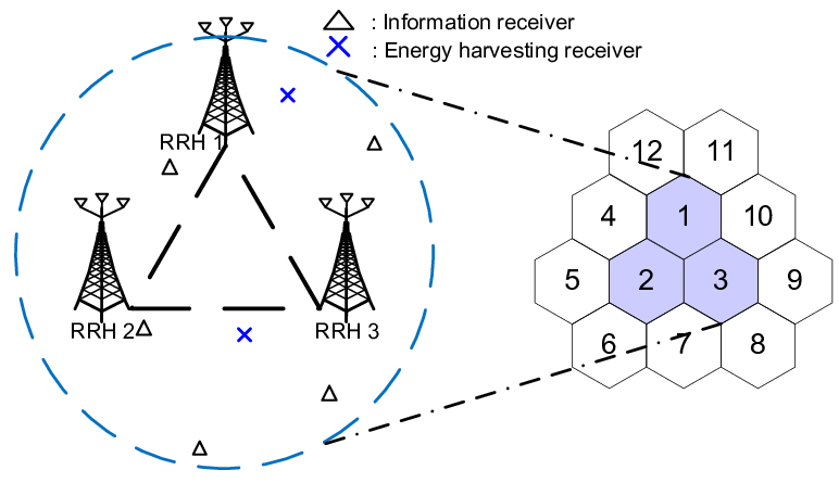
In this section, we evaluate the network performance of the proposed resource allocation algorithms via simulations. We focus on a two-tier distributed antenna network, cf. Figure 3, which includes the impact of multicell interference on the proposed algorithm design. We assume that RRH , , and are connected to the CP, i.e., , to form a cooperative cluster for serving a heavily loaded area in a multicell system (shaded area in Figure 3). There are IRs and ERs in the cooperative cluster. The inter-site distance between any two cooperative RRHs is meters which is a typical distance for a micro-cellular setup. The three cooperative RRHs form an equilateral triangle while the IRs and ERs are uniformly distributed inside a disc with radius meters centered at the centroid of the triangle. The second tier is a lightly loaded area served by RRH – RRH (unshaded area in Figure 3). These RRHs are non-cooperative RRHs each serving the IRs in one of the cells in the second tier. The distance between two neighboring non-cooperative RRHs is meters and each non-cooperative RRH is located at the center of a second tier cell with cell radius meters. In each second tier cell, one IR is uniformly and randomly distributed requiring a minimum SINR of dB and no communication security. Besides, each non-cooperative RRH is powered by a non-renewable energy source and equipped with transmit antennas. Furthermore, the non-cooperative RRHs do not require the backhaul for downlink transmission. The objective of each non-cooperative RRH is to minimize its own transmit power subject to the minimum required SINR constraint. The performance of the proposed algorithms is compared with the performances of a fully cooperative transmission scheme1010 10 Throughout this section, “full cooperation” refers to full cooperation in the first tier of the network. (cooperative transmission and energy cooperation), a fully cooperative transmission scheme with perfect CSI but without (w/o) energy cooperation, and a traditional system with co-located transmit antennas. For the fully cooperation scheme, the solution is obtained by setting , and solving (14) by SDP relaxation. For the fully cooperative scheme with perfect CSI but w/o energy cooperation, we set and , but restrict the cooperative RRHs to not share the harvested energy, and solve (14) by SDP relaxation. For the co-located transmit antenna system, we assume that there is only one cooperative RRH located at the center of the cooperative cluster, which is equipped with the same number of antennas as all first tier cooperative RRHs combined in the distributed stetting, i.e., . Besides, for the co-located transmit antenna system, the CP is at the same location as the RRH and the backhaul is not needed. Furthermore, we set and assume an unlimited energy supply for the co-located transmit antenna system to study its power consumption. Unless specified otherwise, we assume that the maximum SINR tolerance of each ER is set to dB. We adopt an Euclidean sphere for the CSI uncertainty region, i.e., . Furthermore, we define the normalized maximum channel estimation error of ER as , where . The parameters adopted in the simulations are summarized in Table III.
Moreover, we adopt the normalized renewable energy harvesting profile specified in Figure 4, for which the data was obtained at August , in Belgium1111 11 Please refer to http://www.elia.be/en/grid-data/power-generation/ for details regarding the energy harvesting data.. The data is averaged over minutes, i.e., there are sample points per hours. We denote the normalized renewable energy harvesting profile data points for wind energy and solar energy as and , respectively. We follow a similar approach as in [5] to generate the amount of harvested energy at each cooperative RRH for simulation. We assume that the CP has only enough energy to support its circuit power consumption and does not contribute energy to the energy cooperation between the cooperative RRHs. The three cooperative RRHs are equipped with both solar panels and wind turbines with different energy harvesting capabilities. The harvested energy over time at the three cooperative RRHs is given by , , and , respectively, as shown in Figure 5, where Joules is a given constant indicating the maximum available energy from the solar panels and wind turbines. Thus, the maximum harvested energy for cooperative RRH at sample time is given by . The minimum required received SINRs for the five IRs are set to dB, respectively. In case of first tier full cooperation, these five IRs require a total capacity of bit/s/Hz which is the aggregated secrecy rate of all IRs, i.e., .


V-A Convergence of the Proposed Iterative Algorithms
Figure 6 illustrates the convergence of the proposed optimal and suboptimal algorithms for different total numbers of transmit antennas in the network, . The backhaul capacity per link is bits/s/Hz. It can be seen from the upper half of Figure 6 that the proposed optimal algorithm converges to the optimal solution, i.e., the upper bound value meets the lower bound value after less than iterations. On the other hand, the suboptimal algorithm converges to a locally optimal value after less than iterations. We note that if a brute force approach is adopted to obtain a global optimal solution without exploiting the structure of the problem, for IRs and cooperative RRHs, of SDPs need to be solved which may not be computational feasible in practice.


V-B Average Total Transmit Power
In Figure 7, we study the average total transmit power versus the total numbers of transmit antennas in the network, , for different resource allocation schemes. The performances of the proposed optimal and suboptimal iterative algorithms are shown for and iterations, respectively. It can be seen that the transmit power for the proposed optimal and suboptimal schemes decreases when the backhaul capacity per backhaul link increases from bits/s/Hz to bits/s/Hz. This is because the increased backhaul capacity facilitates joint transmission and thus reduces the total transmit power. However, the transmit power of all considered schemes/systems decreases gradually with the total number of transmit antennas in the network. In fact, extra degrees of freedom can be exploited for resource allocation when more antennas are available for the cooperation between the RRHs. Furthermore, the performance gap between the proposed optimal algorithm and fully cooperative transmission is expected to decrease with increasing . For sufficiently large numbers of antennas at the cooperative RRHs, conveying the data of each IR to a subset of cooperative RRHs via the backhaul links may be sufficient for guaranteeing the QoS requirements for reliable communication and efficient power transfer. The lower average total transmit power of fully cooperative transmission with energy cooperation comes at the expense of an exceedingly high backhaul capacity consumption. On the other hand, the proposed suboptimal algorithm achieves an excellent system performance even for the case of only iterations.
Compared to the two proposed schemes, it is expected that the co-located antenna scheme requires a higher transmit power since the co-located antenna system does not offer network type spatial diversity to combat the path loss. Furthermore, Figure 7 reveals that the performance of fully cooperative transmission with perfect CSI and w/o energy cooperation is significantly worse than that of all other schemes. Specifically, cooperative RRH mainly relies on the solar panel for energy harvesting and thus the available energy for cooperative RRH is very limited during the night time. Therefore, despite the availability of perfect CSI and a large number of distributed antennas in the system, the cooperative RRHs having more harvested renewable energy available are required to transmit with comparatively large powers for assisting the cooperative RRHs with smaller harvested renewable energy. In fact, the cooperative RRHs have to cooperate wirelessly which is less power efficient than the cooperation via the micro-grid.
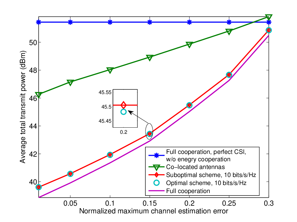
In Figure 8, we show the average total transmit power (dBm) versus the normalized channel estimation error for the proposed schemes with and bits/s/Hz capacity per backhaul link. As can be observed, the average transmit power increases with the normalized channel estimation error except for the case of perfect CSI. The reason behind this is twofold. First, a higher transmit power for the artificial noise, , is required to satisfy constraints C2 and C7 due to a larger uncertainty set for the CSI, i.e., . Second, a higher amount of power also has to be allocated to the information signal , cf. , for neutralizing the interference caused by the artificial noise at the desired IRs.

V-C Average Total Harvested Power
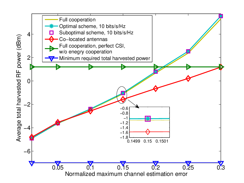
In Figure 9, we study the average total harvested RF power versus the total number of transmit antennas for different resource allocation schemes. It can be observed that the total harvested power of the proposed schemes decreases monotonically with increasing number of transmit antennas. This is because the extra degrees of freedom offered by the increasing number of antennas improve the efficiency of resource allocation. In particular, the direction of beamforming matrix can be more accurately steered towards the IRs which reduces the power allocation to and the leakage of power to the ERs. This also explains the lower harvested power for fully cooperative transmission with energy cooperation which can exploit all transmit antennas in the network for joint transmission. Besides, for the fully cooperative scheme w/o energy cooperation, the ERs harvest the highest amount of power on average at the expense of the highest average total transmit power. Furthermore, although the system with co-located antennas consumes a higher transmit power, it does not always lead to the largest harvested power at the ERs in all considered scenarios. Indeed, a large portion of radiated power in the co-located antenna system is used to combat the path loss which emphasizes the benefits of the inherent spatial diversity in distributed antenna systems for power efficient transmission. We also show in Figure 9 the minimum required total harvested power which is computed by assuming that constraint C7 is satisfied with equality for all ERs. Despite the imperfection of the CSI, because of the adopted robust optimization framework, the proposed optimal and suboptimal resource allocation schemes are able to guarantee the minimum harvested energy required by constraint C7 in every time instant. On the other hand, Figure 10 depicts the average total harvested power versus the normalized channel estimation error for the proposed schemes with and bits/s/Hz backhaul capacity per backhaul link. For imperfect CSI, the harvested power increases with the channel estimation error. In fact, to fulfill the QoS requirements on power transfer and communication secrecy, more transmit power is required for larger which leads to a higher energy level in the RF for energy harvesting.
Remark 5
We note that for all scenarios considered in this section, the proposed resource allocation schemes are able to guarantee the required secrecy rate for all IRs, i.e., , despite the imperfectness of the CSI of the ERs.
VI Conclusions
In this paper, we studied the resource allocation algorithm design for the wireless delivery of both secure information and renewable green energy to mobile receivers in distributed antenna communication systems. The algorithm design was formulated as a non-convex optimization problem with the objective to minimize the total network transmit power. The proposed problem formulation took into account the limited backhaul capacity, the sharing of harvested renewable green energy between RRHs, the imperfect CSI of the ERs, and QoS requirements for secure communication and efficient power transfer. An optimal iterative resource allocation algorithm was proposed for obtaining a global optimal solution based on the generalized Bender’s decomposition. To strike a balance between computational complexity and optimality, we also proposed a low complexity suboptimal algorithm. Simulation results showed that the proposed suboptimal iterative resource allocation scheme performs close to the optimal scheme. Besides, our results unveiled the potential power savings in SWIPT systems employing distributed antenna networks and renewable green energy sharing compared to centralized systems with multiple co-located antennas.
Appendix-Proof of Proposition 1
We start the proof by studying the solution of the dual problem in (24). For a given optimal dual variable , we have
| (38) | |||||
where the first equality is due to the Karush-Kuhn-Tucker (KKT) conditions of the SDP relaxed problem in (19). On the other hand, we can rewrite function as
| (39) | |||||
| (40) |
As a result, the primal solution in the -th iteration, , is also the solution for the minimization in the master problem in (40) for the -th constraint in (29b). Similarly, we can use the same approach to prove that the solution of (28) is also the solution of (31). ∎
References
- [1] D. W. K. Ng and R. Schober, “Resource Allocation for Coordinated Multipoint Networks with Wireless Information and Power Transfer,” in Proc. IEEE Global Telecommun. Conf., Dec. 2014.
- [2] S. Leng, D. W. K. Ng, and R. Schober, “Power Efficient and Secure Multiuser Communication Systems with Wireless Information and Power Transfer,” in Proc. IEEE Intern. Commun. Conf., Jun. 2014.
- [3] “Green Energy Solution by Huawei.” [Online]. Available: {http://www.huawei.com/en/solutions/go-greener/hw-001339-greencommunication-energyefficiency-emissionreduct.htm}
- [4] D. W. K. Ng, E. S. Lo, and R. Schober, “Energy-Efficient Resource Allocation in OFDMA Systems with Hybrid Energy Harvesting Base Station,” IEEE Trans. Wireless Commun., vol. 12, pp. 3412–3427, Jul. 2013.
- [5] J. Xu and R. Zhang, “CoMP Meets Smart Grid: A New Communication and Energy Cooperation Paradigm,” to appear in IEEE Trans. Veh. Technol., Aug. 2014.
- [6] Z. Ding, C. Zhong, D. W. K. Ng, M. Peng, H. A. Suraweera, R. Schober, and H. V. Poor, “Application of Smart Antenna Technologies in Simultaneous Wireless Information and Power Transfer,” IEEE Commun. Mag., vol. 53, no. 4, pp. 86–93, Apr. 2015.
- [7] X. Chen, Z. Zhang, H.-H. Chen, and H. Zhang, “Enhancing Wireless Information and Power Transfer by Exploiting Multi-Antenna Techniques,” IEEE Commun. Mag., no. 4, pp. 133–141, Apr. 2015.
- [8] I. Krikidis, S. Timotheou, S. Nikolaou, G. Zheng, D. W. K. Ng, and R. Schober, “Simultaneous Wireless Information and Power Transfer in Modern Communication Systems,” IEEE Commun. Mag., vol. 52, no. 11, pp. 104–110, Nov. 2014.
- [9] P. Grover and A. Sahai, “Shannon Meets Tesla: Wireless Information and Power Transfer,” in Proc. IEEE Intern. Sympos. on Inf. Theory, Jun. 2010, pp. 2363 –2367.
- [10] R. Zhang and C. K. Ho, “MIMO Broadcasting for Simultaneous Wireless Information and Power Transfer,” IEEE Trans. Wireless Commun., vol. 12, pp. 1989–2001, May 2013.
- [11] D. W. K. Ng, E. S. Lo, and R. Schober, “Wireless Information and Power Transfer: Energy Efficiency Optimization in OFDMA Systems,” IEEE Trans. Wireless Commun., vol. 12, pp. 6352 – 6370, Dec. 2013.
- [12] X. Chen, X. Wang, and X. Chen, “Energy-Efficient Optimization for Wireless Information and Power Transfer in Large-Scale MIMO Systems Employing Energy Beamforming,” IEEE Wireless Commun. Lett., vol. 2, pp. 667–670, Dec. 2013.
- [13] X. Chen, C. Yuen, and Z. Zhang, “Wireless Energy and Information Transfer Tradeoff for Limited-Feedback Multiantenna Systems With Energy Beamforming,” IEEE Trans. Veh. Technol., vol. 63, pp. 407–412, Jan. 2014.
- [14] D. W. K. Ng, E. S. Lo, and R. Schober, “Robust Beamforming for Secure Communication in Systems with Wireless Information and Power Transfer,” IEEE Trans. Wireless Commun., vol. 13, pp. 4599–4615, Aug. 2014.
- [15] L. Liu, R. Zhang, and K.-C. Chua, “Secrecy Wireless Information and Power Transfer with MISO Beamforming,” IEEE Trans. Signal Process., vol. 62, pp. 1850–1863, Apr. 2014.
- [16] D. W. K. Ng and R. Schober, “Max-Min Fair Wireless Energy Transfer for Secure Multiuser Communication Systems,” in Proc. IEEE Inf. Theory Workshop, Nov. 2014, pp. 326–330.
- [17] D. W. K. Ng, E. S. Lo, and R. Schober, “Multi-Objective Resource Allocation for Secure Communication in Cognitive Radio Networks with Wireless Information and Power Transfer,” accept with minor revision, IEEE Trans. Veh. Technol., May 2015.
- [18] D. Lee, H. Seo, B. Clerckx, E. Hardouin, D. Mazzarese, S. Nagata, and K. Sayana, “Transmission and Reception in LTE-Advanced: Deployment Scenarios and Operational Challenges,” IEEE Commun. Mag., vol. 50, pp. 148–155, Feb. 2012.
- [19] R. Irmer, H. Droste, P. Marsch, M. Grieger, G. Fettweis, S. Brueck, H. P. Mayer, L. Thiele, and V. Jungnickel, “Coordinated Multipoint: Concepts, Performance, and Field Trial Results,” IEEE Commun. Mag., vol. 49, pp. 102–111, Feb. 2011.
- [20] D. W. K. Ng, E. S. Lo, and R. Schober, “Energy-Efficient Resource Allocation in Multi-Cell OFDMA Systems with Limited Backhaul Capacity,” IEEE Trans. Wireless Commun., vol. 11, pp. 3618–3631, Oct. 2012.
- [21] J. Zhao, T. Quek, and Z. Lei, “Coordinated Multipoint Transmission with Limited Backhaul Data Transfer,” IEEE Trans. Wireless Commun., vol. 12, pp. 2762–2775, Jun. 2013.
- [22] B. Dai and W. Yu, “Sparse Beamforming for Limited-Backhaul Network MIMO System via Reweighted Power Minimization,” in Proc. IEEE Global Telecommun. Conf., Dec. 2013.
- [23] M. Peng, Y. Li, J. Jiang, J. Li, and C. Wang, “Heterogeneous Cloud Radio Access Networks: A New Perspective for Enhancing Spectral and Energy Efficiencies,” IEEE Wireless Commun., vol. 21, pp. 126–135, Dec. 2014.
- [24] M. Peng, K. Zhang, J. Jiang, J. Wang, and W. Wang, “Energy-Efficient Resource Assignment and Power Allocation in Heterogeneous Cloud Radio Access Networks,” IEEE Trans. Veh. Technol., vol. PP, no. 99, 2014.
- [25] Y. Shi, J. Zhang, and K. Letaief, “Group Sparse Beamforming for Green Cloud-RAN,” IEEE Trans. Wireless Commun., vol. 13, pp. 2809–2823, May 2014.
- [26] G. Zheng, K. K. Wong, and T. S. Ng, “Robust Linear MIMO in the Downlink: A Worst-Case Optimization with Ellipsoidal Uncertainty Regions,” EURASIP J. Adv. Signal Process., vol. 2008, 2008, Article ID 609028.
- [27] B. Zhu, J. Ge, Y. Huang, Y. Yang, and M. Lin, “Rank-Two Beamformed Secure Multicasting for Wireless Information and Power Transfer,” IEEE Signal Process. Lett., vol. 21, pp. 199–203, Feb. 2014.
- [28] Q. Li, W.-K. Ma, and A.-C. So, “Robust Artificial Noise-Aided Transmit Optimization for Achieving Secrecy and Energy Harvesting,” in Proc. IEEE Intern. Conf. on Acoustics, Speech and Signal Process., May 2014, pp. 1596–1600.
- [29] G. Geraci, S. Singh, J. Andrews, J. Yuan, and I. Collings, “Secrecy Rates in Broadcast Channels with Confidential Messages and External Eavesdroppers,” IEEE Trans. Wireless Commun., vol. 13, pp. 2931–2943, May 2014.
- [30] A. J. Wood and B. F. Wollenberg, Power Generation, Operation, and Control. Wiley-Interscience.
- [31] K.-Y. Wang, A.-C. So, T.-H. Chang, W.-K. Ma, and C.-Y. Chi, “Outage Constrained Robust Transmit Optimization for Multiuser MISO Downlinks: Tractable Approximations by Conic Optimization,” IEEE Trans. Signal Process., vol. 62, pp. 5690–5705, Nov. 2014.
- [32] J. Yang and S. Ulukus, “Optimal Packet Scheduling in an Energy Harvesting Communication System,” IEEE Trans. Commun., vol. 60, pp. 220–230, Jan. 2012.
- [33] R. Ramamonjison, A. Haghnegahdar, and V. Bhargava, “Joint Optimization of Clustering and Cooperative Beamforming in Green Cognitive Wireless Networks,” IEEE Trans. Wireless Commun., vol. 13, pp. 982–997, Feb. 2014.
- [34] C. A. Floudas, Nonlinear and Mixed-Integer Optimization: Fundamentals and Applications, 1st ed. Oxford University Press, 1995.
- [35] D. Li and X. Sun, Nonlinear Integer Programming. Springer, 2006.
- [36] S. Boyd and L. Vandenberghe, Convex Optimization. Cambridge University Press, 2004.
- [37] M. Grant and S. Boyd, “CVX: Matlab Software for Disciplined Convex Programming, version 2.0 Beta,” [Online] https://cvxr.com/cvx, Sep. 2013.
- [38] “MOSEK ApS: Software for Large-Scale Mathematical Optimization Problems, Version 7.0.0.111,” Apr. 2014. [Online]. Available: http://www.mosek.com/
- [39] “GUROBI Optimization, State-of-the-Art Mathematical Programming Solver, v5.6,” Apr. 2014. [Online]. Available: http://www.gurobi.com/
- [40] A. M. Geoffrion, “Generalized Benders Decomposition,” J. Optimization Theory Appl., vol. 10, pp. 237–260, Feb. 1972.
- [41] E. Che, H. Tuan, and H. Nguyen, “Joint Optimization of Cooperative Beamforming and Relay Assignment in Multi-User Wireless Relay Networks,” IEEE Trans. Wireless Commun., vol. 13, pp. 5481–5495, Oct. 2014.
- [42] Q. T. Dinh and M. Diehl, “Local Convergence of Sequential Convex Programming for Nonlinear Programming,” in Chapter of Recent Advances in Optimization and Its Application in Engineering. Oxford University Press, 2010.
- [43] I. Pólik and T. Terlaky, “Interior Point Methods for Nonlinear Optimization,” in Nonlinear Optimization, ser. Lecture Notes in Mathematics, G. Di Pillo and F. Schoen, Eds. Springer Berlin Heidelberg, 2010, pp. 215–276.
- [44] T. H. Cormen, C. E. Leiserson, R. L. Rivest, and C. Stein, Introduction to Algorithms, 3rd ed. The MIT Press, 2009.
- [45] B. Choi and G. Lee, “New Complexity Analysis for Primal-Dual Interior-Point Methods for Self-Scaled Optimization Problems,” Fixed Point Theory and Applications, no. 1, p. 213, Dec. 2012.
- [46] G. Wang and Y. Bai, “A New Primal-Dual Path-Following Interior-Point Algorithm for Semidefinite Optimization,” Journal of Mathematical Analysis and Applications, vol. 353, pp. 339 – 349, 2009.