Power Allocation with Stackelberg Game in Femtocell Networks: A Self-Learning Approach
Abstract
This paper investigates the energy-efficient power allocation for a two-tier, underlaid femtocell network. The behaviors of the Macrocell Base Station (MBS) and the Femtocell Users (FUs) are modeled hierarchically as a Stackelberg game. The MBS guarantees its own QoS requirement by charging the FUs individually according to the cross-tier interference, and the FUs responds by controlling the local transmit power non-cooperatively. Due to the limit of information exchange in intra- and inter-tiers, a self-learning based strategy-updating mechanism is proposed for each user to learn the equilibrium strategies. In the same Stackelberg-game framework, two different scenarios based on the continuous and discrete power profiles for the FUs are studied, respectively. The self-learning schemes in the two scenarios are designed based on the local best response. By studying the properties of the proposed game in the two situations, the convergence property of the learning schemes is provided. The simulation results are provided to support the theoretical finding in different situations of the proposed game, and the efficiency of the learning schemes is validated.
I Introduction
Femtocells are considered to be an efficient and economic solution to enhance the indoor experience of the cellular mobile users [1]. A femtocell is a low-power, short-range access point, which can be quickly deployed by the end-users. It provides better spatial reuse of the spectrum by serving the nearby users who have poorer connections with the Macrocell Base Station (MBS) due to penetration loss. In practice, the femtocell network usually operates underlaying the macrocell network. This is mainly due to the ad-hoc topology of the femtocells and thus the lack of coordination between the MBS and Femto Access Points (FAPs). Consequently, inter-cell/cross-tier interference arises, and interference mitigation becomes necessary for preventing performance deterioration.
Due to the ad-hoc topology of the femtocells, the FAP deployment faces the limited information exchange both across tiers and among the femtocells. Therefore, it is desirable that the interference management of the femtocells is fully distributed, and each Femtocell User (FU) is capable of adapting to the surrounding environment with minimum information. With this in mind, we study the power control schemes for a shared-spectrum, two-tier femtocell network. We note that the Macrocell User (MU) prefers that the cross-tier interference is minimized, while the FUs prefers to transmit with the best Signal-to-Interference-plus-Noise-Ratio (SINR). Considering that private objectives contradict with each other, it is natural to introduce the tools of game theory and model the cross-tier, self-centric interactions in the framework of non-cooperative games.
I-A Related Work
Under the framework of non-cooperative games, the early study [2] has discovered that power control purely based on the non-cooperative games will lead to inefficient equilibria. In order to obtain the Pareto-preferred equilibria, a number of approaches including the introduction of repetition [3] or externalities (e.g., pricing) [4, 5] are adopted in the research. As shown by studies in non-hierarchical networks [4, 5, 6], choosing a proper pricing mechanisms with respect to different utility functions can be an efficient way of determining the desired properties of the equilibria.
When it comes to the resource allocation in hierarchical networks, such as the femtocell networks and cognitive radio networks, the Stackelberg game [7] based modeling is widely preferred since it is able to reflect the features of hierarchy and ad-hoc topology in the network [8, 9]. the Stackelberg game is characterized by the sequential decision making manner (namely, the follower-leader strategy updating), and hence suitable for modeling the heterogeneous user behaviors in the network. Due to the computational intensity for obtaining the Stackelberg Equilibrium (SE), most of the existing studies [9, 10, 11] adopt a utility model that favors the derivation of a closed-form SE, and solve for the SEs through transforming the games as hierarchical optimization problems.
Although the optimization-technique-based methods are able to precisely analyze the properties of the SEs, their scope is limited to the games with a certain categories of utility functions. Beyond those games, a natural idea is to resort to tools of iterative learning in repeated games for searching the SEs. A body of literature on non-hierarchical networks can be found applying iterative strategy-learning methods [12, 13], usually based on the assumption of the discrete strategy space [14]. However, since these learning methods assume homogeneous behaviors among the players, most of their application to hierarchical networks are also limited within an uniform learning model [15, 16].
I-B Self-Learning under Pricing
In this paper, we model the power allocation problem in the two-tier femtocell network from the perspective of the Stackelberg game. In the game, the MBS behaves as the leader and controls the total cross-tier interference by setting prices to each FU-FAP link. The FU-FAP links behave as the followers to optimize their energy efficiency through interactive power allocation. In designing the distributed, hierarchical power control scheme with pricing, the power efficiency is adopted as the utility of the FU-FAP link. we investigate the scenarios of the continuous and discrete power profile of the femtocells, respectively. Due to the computational complexity of obtaining the closed-form solution of the equilibrium, we investigate the property of the game in the two situations, and propose two self-centric strategy-learning algorithms for the follower game based on the local myopic best response, respectively. We provide the theoretical proof of the convergence of the learning schemes. Also, we provide two heuristic algorithms for obtaining the optimal MBS prices in the corresponding situations. In the simulation, we provide the experimental comparison on the network performance between the two scenarios, and demonstrate the efficiency of the proposed learning algorithms.
II Problem Formulation
II-A Network Model
We consider the uplink transmission of a two-tier femtocell network with a single MBS and FAPs. The MBS and the FAPs share the same bandwidth and each of them is scheduled to serve one single user at each time instance. The MBS is required to keep the femtocell-to-macrocell interference to an acceptable level. Due to the ad-hoc topology of the femtocells, we assume that the information exchange only happens between the MBS and FAPs. For analytical tractability, we suppose that all the channels involved are block-fading and remains constant during each transmission block.
In what follows, we let denote the index of the MU-MBS pair and denote the index of a FU-FAP pair. The channel power gain between the transmitter of pair and the receiver of pair is denoted by , where . The power of transmitter is denoted by and the power vector of all the FUs is denoted by . The noise variance for the transmitter-receiver pair is denoted by . Then the SINR level at the MBS can be expressed as:
| (1) |
and the SINR level at the -th FAP can be expressed as
| (2) |
During the operation, it is usually beneficial to shift some calls served by the MBS to the FAP. Therefore, we suppose that for the MBS, the requirement on the femtocell-to-macrocell interference is not rigid. Instead, the MU transmit with a fixed power and the MBS charges each FU-FAP link for causing interference with a certain price to control the interference level. We denote the vector of interference prices at a time interval by , in which is the price for unit interference caused by FU . The goal of the MBS is to maximize the total revenue of collecting payments from the FU-FAP links:
For simplicity, in what follows we use the terms FU and the FU-FAP link interchangeably. For the FUs, we assume that each local transmit power is limited by the physical constraint . The goal of FU is to maximize its local net payoff by adapting :
| (5) |
in which is the utility function of FU . Considering the practical scenarios, we adopt the local utility as the energy efficiency (namely, the data received per unit energy consumption) of each FU:
| (6) |
where denotes the additional circuit power consumption for FU . We assume that the local SINR can be perfectly measured at the FAP. For the proposed femtocell network, we suppose that the following assumptions hold:
- i)
is significantly greater than ;
- ii)
The femtocell-to-femtocell interference is sufficiently small.
Assumption i) is based on the fact that most power is consumed during operation by the amplifier and the radio transceiver [17]. Assumption ii) is based on the practical concerns that (a) the FAPs are of low power, so the peak transmit power is limited; and (b) the intercell gains between femtocells are usually weak due to the path loss (since the indoor penetration loss is usually significant). Based on the assumptions, we assume that the SINR constraint for a FU-FAP link is negligible.
III Stackelberg Game Analysis
We model the user interactions in the proposed network as a hierarchical game with the MBS and the FU-FAP links choosing their actions in a sequential manner. When the power allocation of the FUs are given as , we can define the leader game from the perspective of the MBS as:
| (7) |
in which the MBS is the only player of the game and the action of the player is the price vector .
When the leader action is given by , we can define the non-cooperative follower game from the perspective of the FUs as:
| (8) |
in which FU is one player with the local action .
With each player behaving rationally, the goal of the game (7) and (8) is to finally reach the Stackelberg Equilibrium (SE) in which both the leader (MBS) and the followers (FUs) have no incentive to deviate. We first assume that the strategies of the FUs and MBS are continuous. Then the SE of the game can be mathematically defined as follows:
Definition 1 (Stackelberg Equilibrium).
III-A Femtocell Power Allocation with Continuous Strategies
We start the analysis of the Stackelberg game in (7) and (8) by back induction. Suppose that the MBS first sets its strategy as , then we obtain the non-cooperative follower subgame described by (8). In order to show the existence of a pure-strategy Nash Equilibrium (NE) in , we introduce the concept of supermodular game as follows.
Definition 2 (Supermodularity[7]).
A function is said to have increasing differences (supermodularity) in if for all and ,
Definition 3 (Supermodular game [7, 18]).
A general normal-form game is a supermodular game if for any player ,
- i)
the strategy space is a compact subset of .
- ii)
the payoff function is upper semi-continuous in .
- iii)
is supermodular in and has increasing difference between any component of and any component of .
Theorem 1.
Given the strategy of the MBS, the follower subgame (8) is a supermodular game if .
Proof.
See Appendix A. ∎
Given the opponent strategies , we define the local Best Response (BR) of FU by
| (11) |
Proposition 1.
At least one pure-strategy NE exists in the follower subgame (8) and the following points hold:
- i)
The set of NEs (10) has the component-wise greatest element and least element .
- ii)
If the BRs are single-valued, and each FU uses the BR starting from the smallest (largest) elements of the strategy space to update their strategies, then the strategies monotonically converge to the smallest (largest) NE.
- iii)
If the game has a unique NE, then with any arbitrary initial strategy, the local myopic BRs converges to the NE.
The properties of in Proposition 1 sheds light on the solution to the local strategy-learning scheme for the FUs. To take advantages of these properties, we first examine the BRs in and obtain Lemma 1:
Lemma 1.
Given the MBS strategy , is strictly quasiconcave and the best-response is single-valued for each FU.
Proof.
See Appendix B. ∎
Based on Lemma 1, we can further prove that the BR of FU has the following properties, and therefore is a standard function [7]:
- i)
positivity: ,
- ii)
monotonicity: for any , if , then ,
- iii)
scalability: , .
Based on the aforementioned properties, we can directly apply the results in [7] and deduce the uniqueness of the pure-strategy NE in the follower subgame .
Theorem 2.
Given any MBS strategy , the follower subgame (8) has a unique NE if the following condition is satisfied
| (12) |
Proof.
See Appendix C. ∎
Remark 1.
If in subgame the condition of Theorem 2 is satisfied, the condition of Theorem 1 will also be satisfied. (12) indicates that to ensure the uniqueness of the NE, the SINR of a FU should be significantly larger than the ratio between its transmit power and circuit power. Such a condition is guaranteed by our assumption of the network.
We assume that the channel power gain is known and the SINR can be perfectly measured by each FAP. Then, based on Lemma 1, can be solved locally with the bisection method [19]. Based on Proposition 1 and Theorem 2, the asynchronous strategy-updating mechanism defined in [18] can be directly applied to . By Proposition 1, the convergence to the NE is guaranteed from any arbitrary initial power vector. The strategy-learning algorithm is summarized as Algorithm 1:
III-B Approximate Solution to the Price of MBS
When considering the leader subgame , we assume that the strategies of the FUs are given as from (11). For the subgame (7), the local BR is given by
| (13) |
To investigate the solution of (13), we first consider the feasible region of . We note from (11) that the maximum value of is lower-bounded by (when ) and upper-bounded by , in which . Thereby, the price charged by the MBS is also upper-bounded. Otherwise, if is too high (i.e., making ), FU will stop transmitting and be forced out of the game. With the aforementioned bound on , we look for the constraint on in (11). However, since in (11) is a transcendental function, it is difficult to derive a closed-form expression of the constraint on . Then, the challenge of analyzing is to find an efficient way for obtaining the optimal price .
By jointly investigating the leader and the follower subgames, we can show that a finite, optimal price for each FU coexists with the NE of the follower subgame.
Theorem 3.
Proof.
The proof is based on Theorem 3.2 of [7]. Given the condition that each local strategy in the game is compact and convex and the corresponding payoff function is quasiconcave, the existence of a pure-strategy SE is guaranteed. For the FUs, quasiconcavity of in is given by Lemma 1. For the MBS, is an affine function of , hence being quasiconcave in . It is trivial that and are convex and compact, then based on Theorem 3.2 of [7], there exists a pure-strategy NE in the game. Beyond the discussion after (13) on the fact that , we can derive the relationship of the BRs between the FUs and the MBS from as:
| (14) |
in which and are the local BR and the corresponding SINR. is given by (31) in Appendix A. For (14), the value of the right-hand side expression is upper-bounded since . Then is finite. ∎
Our approximate solution to the leader subgame is inspired by the pioneering work of [4], which models the asymptotic behaviors of the equilibriu bhum power vector and the corresponding payments. We assume that each FU’s behavior can be asymptotically modeled by two regions, the price-insensitive region and the price-sensitive region. In the price-insensitive region, the FU’s behaviors are hardly influenced by the price. In the price-sensitive region, the local power allocation is driven toward 0. Mathematically, the two-region model can be expressed by the following asymptotes:
- •
Low-price asymptote as :
(15) - •
High-price asymptote as :
(16)
In (15), is the equilibrium SINR when . The details for deriving (15) and (16) is presented in Appendix D. Since in the low-price asymptote, increases with and in the high-price asymptote it decreases with , the maximum payment must happen between the two regions. Then, we can extend the two FU payment asymptotes toward each other until they meet at the intersection price . With such an approximation, will be the maximum payment received from FU . Combining (15) and (16), we can obtain the intersection point for the two asymptotes as:
| (17) |
in which is the power allocation corresponding to the SINR in (15). It can be obtained by setting and solving (44) with the BR-based asynchronous strategy-updating mechanism.
III-C Femtocell Power Allocation in Discrete Strategies
We continue to extend the analysis of the game to the scenario in which the FUs choose their strategies from a finite, discrete set of powers. In this case, the conditions for NEs (i.e., Theorems 2 and 3) are not satisfied anymore. Therefore, the properties of the NE need to be re-evaluated. Within the same game structure of (7) and (8), we denote the action set of the FUs by . It is well known that every finite non-cooperative game has a mixed-strategy NE [7]. For the follower subgame, we define the mixed-strategies of FU as , in which is the probability for FU to choose the -th action . Then, given any MBS price , there will be at least one mixed-strategy NE for the FUs. Different from the continuous game, the expected net payoff of FU becomes
| (18) |
in which . Similarly, the expected revenue of the MBS becomes
| (19) |
Due to the limit of information exchange, FU can only attain its local payoff each time when it chooses and the other FUs adopt the mixed strategies . To ensure that each FU is able to learn its Nash distribution , we adopt the Logit best response function (namely, the smooth BR based on entropy perturbation) [20]:
| (20) |
in which is the estimated expected payoff at time . is a positive scalar (also known as Boltzmann temperature) that controls the sensitivity of the BR to perturbation.
Based on the two-timescale strategy learning scheme [20], we introduce two coupled stochastic learning processes to approximate and in (20) as follows:
| (21) | ||||
| (22) |
In (21) and (22), is the instant payoff observation at the FAP in (5) and is the smooth BR (20). is the indicator function. if and otherwise . The parameter sequence and satisfy the following conditions:
The conditions in (III-C) ensures that the learning of strategies changes on a slower timescale than that of the action values. Based on the discussion in [21], we can show that the learning processes converges by Theorem 4:
Theorem 4.
Proof.
See Appendix E. ∎
In the scenario of finite strategies, it is even more difficult to obtain a SE point for the MBS prices. However, by investigating the property of concavity in the payoff function for any element or of the joint strategy vector , we can show that there exists at least one SE with MBS price in pure-strategy:
Theorem 5.
Proof.
The proof for the existence of the SE follows directly from Theorem 1 of [22]. It is easy to see that the payoff function is linear (hence concave) in if and the rest of the elements of are fixed. Similarly, is linear in with and fixed. Therefore, following the discussion of Theorem 1 in [22] and the Kakutani fixed point theorem, there exists a fixed point satisfying Definition 1.
The proof of a finite in the SE is similar to that in Theorem 3. If we assume that is a SE, then from (18) we obtain ,, which is equivalent to
| (27) |
Similar to the continuous-game scenario in Theorem 3, it is easy to verify that as , and . We note that , the equation array (27) always has a solution since the mixed-strategy NE exists. With (19) and (27), we can obtain
| (28) |
which must have a non-zero maximum value. Therefore, we can always find a finite that maximize (19) with the NE of the follower game, Otherwise, it will contradict with the fact that as . ∎
Following our discussion, we propose a pricing mechanism based on the myopic best response as Algorithm 2:
IV Simulation Results
The objective of this section is to provide insight into the impact of pricing on the network performance at the equilibrium, and the influence of strategy discretization on the learning process. In the simulation, we assume that the FAPs are randomly located indoors within a circle centered at the MBS with a radius of m. Each FU is placed within a circle centered at the corresponding FAP with a radius of m. The channel gains of the transmitter-receiver pairs are generated by a lognormal shadowing pathloss model with , in which is the pathloss factor, for the FUs and for the MU. The parameters used in the simulation are summarized in Table I.
| Parameter | Value |
|---|---|
| Shared Bandwidth | 1MHz |
| Maximum MU transmit power | dBm |
| Feasible region for FU transmit power | dBm |
| Additional FU circuit power | dBm |
| AWGN power | dBm |
| SINR threshold of the MU | 3dB |
IV-A Analysis of the Equilibrium in the Continuous Game
In the first simulation, we study the influence of the MBS price on the equilibrium of the follower subgame with 6 FAPs. For the convenience of demonstration, we suppose that the MBS charges an identical price to each FU-FAP link. Figure 1 provides the payoffs evolution of both the MBS and the FU-FAP links at the follower-game NE as the uniform price increases. We note in Figure 1.b that there exists an optimal value of to maximize the MBS revenue, which provides an experimental evidence of Theorem 3. We also note from Figure 1.a and 1.b that there exists a plateau region in which the average power efficiency remains almost the same while the MBS revenue keeps increasing. It means that without undermining the social welfare of the femtocells, the MBS is able to control the cross-tier interference by choosing the price within the plateau region.
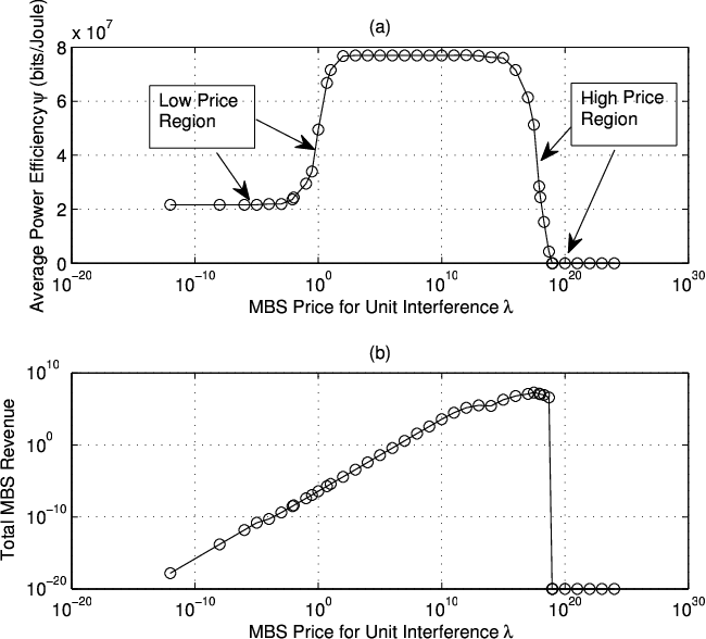
We note from Figure 1 that at the optimal MBS price (i.e., the SE point), the FU performance dramatically degrades from the optimal condition. This leaves the room in practice for the MBS to trade a portion of the revenue for a socially better performance. Following the first simulation, we investigate the network performance at the proposed price (17) as the number of FAPs varies. In Figures 2 and 3, the user performance at the proposed price is compared to that at the accurate SE price, and that with no price (). The accurate SE price is obtained using a semi-exhaustive searching method with bisection, and the utilities are obtained from Monte Carlo simulation. Figure 2 shows that at the proposed price a better FU performance can be achieved (Figure 2.b) at the cost of losing a significant portion of the MBS revenue (Figure 2.a). However, by measuring the expected SINR of the MU in Figure 3, we note that such trade-off is worthwhile since the performance deterioration of the MU is small when compared to the gain of the FU performance. Again, Figure 2.b and Figure 3 shows the fact that with no externality, the network performance can be heavily impaired (see curve “No price, ”).


IV-B Analysis of the Equilibrium in Discrete Game
Since we are interested in the impact of strategy discretization on the network performance, we adopt the same network setup in the first simulation for the discrete game. The parameter for the self-learning algorithm is given in Table II. To compensate for the divergence caused by the self-learning algorithm (Theorem 4), we examine the expected user utilities with Monte Carlo simulation. For the convenience of demonstration, we also suppose that the MBS places an uniform price. The simulation results are shown in Figure 4.
| Parameter | Value |
|---|---|
| Boltzmann temperature | 1 |
| Learning rate for and | and |
| Number of candidate power | |
| Power sampling equation |
Figure 4.b shows the existence of an optimal that maximizes the MBS revenue. It can be interpreted as an experimental evidence of Theorem 5. Comparing Figure 4.a and Figure 1.a, we note that in the discrete follower game (Figure 4.a), the “plateau” region extends to . It means that different from the case of continuous game (Figure 1.a), lacking an external price does not severely undermine the social performance of the FUs. However, the femtocell network may suffer from discretization of the power space and only achieve approximately of the performance in the continuous game at most of the NEs.
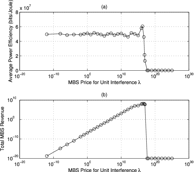
Figure 5 shows the user performance at the proposed price with Algorithm 2, the accurate SE price and zero price, respectively. The comparison in Figure 5 shows that the FU performance at the proposed price is the best of the three. However, from Figure 5.b we note that without a pricing scheme, the FUs can still achieve a good performance level. As the number of FAPs increases, we can observe a deterioration in the FU performance. It means that mixed-strategies NE in the discrete game is not as good as the continuous-game NE in maintaining the performance when the size of network increases (see Figure 2.b).

Finally, we demonstrate in Figures 6 and 7 the convergence of the self-learning algorithm in the discrete game of FUs. Figure 6 shows a snapshot of FUs’ transmit-power evolution during the learning process of Algorithm 2. Figure 7 shows the corresponding strategy evolution of FU 1. By running the simulation for multiple times, we observe that most of the learning processes converge within iterations.


V Conclusion
In this paper, we have formulated the price-based power allocation problem in the two-tier femtocell network under the framework of the Stackelberg game. We have provided the theoretical analysis of the properties of the equilibria in the scenarios of continuous FU power space and discrete power space, respectively. We have proposed two self-sufficient learning algorithms, one for each situation, for learning the NE of the follower game with limited information exchange. We have also provided the theoretical proof for the convergence of the learning algorithms. Our simulation results provides important insight in the different impact of the pricing mechanism on the network performance in the scenarios of the continuous game and the discrete game. In the simulation, we also show the efficiency of the proposed heuristic price-searching mechanism in the game. Our study provides an alternative way of designing the resource allocation protocols since no intercell information exchange is required in the femtocells.
Appendix A Proof of Theorem 1
Lemma 2 ([18]).
If a function is twice differentiable, then supermodularity is equivalent to , .
The first and the second conditions of a supermodular game in Definition 3 (trivially) holds for the proposed follower subgame (8). Then, Theorem 1 can be derived based on Lemma 2. By taking the component-wise derivative of with respect to , we obtain:
| (30) |
in which
| (31) |
Then , , the value of is given by:
| (32) |
in which
| (33) |
It is easy to verify from (32) that if . By Lemma 2, has increasing difference between and any component of if . By Definition 3, the proof of Theorem 1 is completed.
Appendix B Proof of Lemma 1
The proof of Lemma 1 is derived from investigating the quasiconcavity of the FU payoff functions. For conciseness, the readers are referred to Sections 3.1 and 3.4 of [19] for the details of the definition in superlevel set and quasiconcavity.
Lemma 3 ([19]).
Suppose be strictly quasiconcave where is convex. Then any local maximum of on is also a global maximum of on . Moreover, the set is either empty or a singleton.
We first show that the utility function in is quasiconcave. We examine the -superlevel set of in , which is equivalent to the 0-superlevel set of :
| (34) |
We note that is a concave function, so is convex by the definition of convexity. By the definition of quasiconcavity, is quasiconcave in .
Then we show that is strictly quasiconcave in so the BR is a global maximum and thus single-valued. Without loss of generality, we consider the power allocation with . We assume that a different power allocation satisfies . Correspondingly, and . Observing the following condition for :
| (35) |
in which is given in (31). We note that the right-hand side of (35) is a strictly increasing concave function and the left-hand side is a strictly increasing convex function in . Then the solution to is unique in , so . Based on the definition of concave function, the following inequality also holds for :
| (36) |
Therefore, the condition for strict quasiconcavity holds as . Then Lemma 1 is a direct conclusion based on Lemma 3.
Appendix C Proof of Theorem 2
Lemma 4 ([7]).
If the best-response functions of a non-cooperative game are standard functions for all the players, then the game has a unique NE in pure strategies.
Observing (5), we note that the maximum net-payoff function is lower-bounded by 0 with . Since the power vector is always nonnegative, the property of positivity in the BR for each FU immediately follows Lemma 1.
We denote . Noting that is a strictly increasing function of , monotonicity of can be illustrated by proving that function is monotonically increasing in . From (30) we obtain the necessary condition for to be the BR as , which is equivalent to
| (37) |
Since , we have
| (38) |
in which , and
| (39) |
in which . We note that , then the property of monotonicity holds iff . With the inequality of logarithmic function [23], for , we obtain
| (40) |
Therefore, if . Then we obtain the condition for to be monotonic as:
| (41) |
The proof of scalability is based on Lemma 1. According to Lemma 1, there is a one-to-one correspondence between and . We define , then from (2) the BR can be written as
| (42) |
From , we can prove that with the same technique as proving monotonicity (which is omitted for conciseness). Therefore, is a decreasing function of . Since is a standard function [18], we realize that if , and . Then, monotonicity holds for since
| (43) |
Therefore, is a standard function. Based on Lemma 4, the NE of the follower subgame (8) is unique.
Appendix D The Derivation of Asymptotic Behavior Models
Appendix E Proof of Theorem 4
Lemma 5 ([21]).
Consider game with payoff function for player . If the sequence of stochastic fictitious play converges, it also holds for game with payoff function , in which is a positive constant and only depends on player ’s own behavior.
Lemma 6 ([21]).
Consider stochastic fictitious play starting from any arbitrary . If is a supermodular game, then
where is an invariant set of the solution trajectory starting from . is the set of rest points (fixed points) and such that . is a finite Lipschitz submanifold and every persistent non-convergence trajectory is asymptotic to one in .
The proof of Theorem 4 starts by investigating the property of supermodularity in the FU subgame. With discrete power set, the expected payoff function (18) can be rewritten as:
| (48) |
which is in the form with . By Lemma 5, we only need to check the game with payoff
| (49) |
With Definition 3 and Lemma 2, it is easy to check that the game with payoff function (49) and mixed strategies is a supermodular game. Based on Theorem 6 of [20], the process of produced by (20)-(22) will almost surely be an asymptotic pseudotrajectory of the smooth BR dynamics:
Then, based on Lemma 6, for the game with payoff (49) stochastic fictitious play almost surely converges with any arbitrary initial . With Lemma 5, the convergence holds for the original subgame with payoff , so Theorem 4 is proved.
References
- [1] J. Andrews, H. Claussen, M. Dohler, S. Rangan, and M. Reed, “Femtocells: Past, present, and future,” IEEE J. Sel. Areas in Commun., vol. 30, no. 3, pp. 497–508, Apr. 2012.
- [2] C. Saraydar, N. B. Mandayam, and D. Goodman, “Efficient power control via pricing in wireless data networks,” IEEE Trans. on Commun., vol. 50, no. 2, pp. 291–303, Feb. 2002.
- [3] A. MacKenzie and S. Wicker, “Game theory in communications: motivation, explanation, and application to power control,” in Proc. IEEE GLOBECOM, vol. 2, San Antonio, TX, Dec. 2001, pp. 821–826.
- [4] N. Feng, S.-C. Mau, and N. B. Mandayam, “Pricing and power control for joint network-centric and user-centric radio resource management,” IEEE Trans. on Commun., vol. 52, no. 9, pp. 1547–1557, Sep. 2004.
- [5] H. Yu, L. Gao, Z. Li, X. Wang, and E. Hossain, “Pricing for uplink power control in cognitive radio networks,” IEEE Trans. Veh. Tech., vol. 59, no. 4, pp. 1769–1778, May 2010.
- [6] J. Huang, R. Berry, and M. Honig, “A game theoretic analysis of distributed power control for spread spectrum ad hoc networks,” in Proc. Inter. Sym. Info. Thm., Adelaide, Australia, Sep. 2005, pp. 685–689.
- [7] Z. Han, D. Niyato, W. Saad, T. Basar, and A. Hjorungnes, Game theory in wireless and communication networks. Cambridge University Press, 2012.
- [8] J. Zhang and Q. Zhang, “Stackelberg game for utility-based cooperative cognitiveradio networks,” in Proc. ACM MobiHoc, New York, NY, May 2009, pp. 23–32.
- [9] X. Kang, R. Zhang, and M. Motani, “Price-based resource allocation for spectrum-sharing femtocell networks: A stackelberg game approach,” IEEE J. Sel. Areas Commun., vol. 30, no. 3, pp. 538–549, Apr. 2012.
- [10] Y. Wu, T. Zhang, and D. H. K. Tsang, “Joint pricing and power allocation for dynamic spectrum access networks with stackelberg game model,” IEEE Trans. Wireless Commun., vol. 10, no. 1, pp. 12–19, Jan. 2011.
- [11] L. Yang, H. Kim, J. Zhang, M. Chiang, and C.-W. Tan, “Pricing-based spectrum access control in cognitive radio networks with random access,” in Proc. IEEE INFOCOM, Shanghai, China, Apr. 2011, pp. 2228–2236.
- [12] P. Zhou, Y. Chang, and J. Copeland, “Reinforcement learning for repeated power control game in cognitive radio networks,” IEEE J. Sel. Areas Commun., vol. 30, no. 1, pp. 54–69, Jan. 2012.
- [13] A. Galindo-Serrano, L. Giupponi, and M. Dohler, “Cognition and docition in ofdma-based femtocell networks,” in Proc. IEEE GLOBECOM, Miami, FL, Dec. 2010, pp. 1–6.
- [14] C. Long, Q. Zhang, B. Li, H. Yang, and X. Guan, “Non-cooperative power control for wireless ad hoc networks with repeated games,” IEEE J. Sel. Areas Commun., vol. 25, no. 6, pp. 1101–1112, Aug. 2007.
- [15] M. Bennis, S. Perlaza, P. Blasco, Z. Han, and H. Poor, “Self-organization in small cell networks: A reinforcement learning approach,” IEEE Trans. Wireless Commun., vol. 12, no. 7, pp. 3202–3212, Jul. 2013.
- [16] X. Chen, H. Zhang, T. Chen, and M. Lasanen, “Improving energy efficiency in green femtocell networks: A hierarchical reinforcement learning framework,” in Proc. IEEE ICC., Budapest, Hungary, Jun. 2013, pp. 2241–2245.
- [17] C. Han, T. Harrold, S. Armour, I. Krikidis, S. Videv, P. M. Grant, H. Haas, J. Thompson, I. Ku, C. Wang, T. A. Le, M. Nakhai, J. Zhang, and L. Hanzo, “Green radio: radio techniques to enable energy-efficient wireless networks,” IEEE Commun. Mag., vol. 49, no. 6, pp. 46–54, Jun. 2011.
- [18] E. Altman and Z. Altman, “S-modular games and power control in wireless networks,” IEEE Trans. Auto. Ctrl., vol. 48, no. 5, pp. 839–842, May 2003.
- [19] S. P. Boyd and L. Vandenberghe, Convex optimization. Cambridge university press, 2004.
- [20] D. S. Leslie and E. Collins, “Convergent multiple-timescales reinforcement learning algorithms in normal form games,” Ann. Appl. Probab., vol. 13, no. 4, pp. 1231–1251, Feb. 2003.
- [21] J. Hofbauer and W. H. Sandholm, “On the global convergence of stochastic fictitious play,” Econometrica, vol. 70, no. 6, pp. 2265–2294, Nov. 2002.
- [22] J. B. Rosen, “Existence and uniqueness of equilibrium points for concave n-person games,” Econometrica, vol. 33, no. 3, pp. pp. 520–534, 1965.
- [23] F. Topsok, “Some bounds for the logarithmic function,” in Inequality theory and applications, vol. 7, no. 2. Nova Science Pub Incorporated, 2006, pp. 137–156.