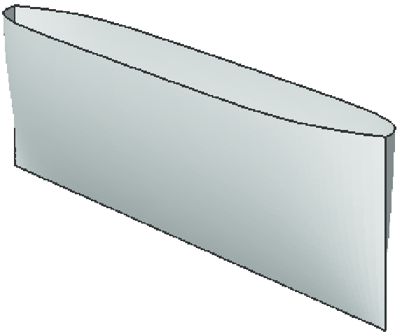
跳到论文正文
W Papers独立论文阅读器 arXiv:1410.2800 论文正文 计算阅读时间 · 0%
引用这篇论文根据当前论文元数据生成,正式投稿前建议核对。


License: arXiv.org perpetual non-exclusive license
arXiv:1410.2800v1 [math.OC] 10 Oct 2014

A theoretical and numerical determination of optimal ship forms based on Michell’s wave resistance

Julien Dambrine and Morgan Pierre and Germain Rousseaux Address: Julien Dambrine and Morgan Pierre, Université de Poitiers, Laboratoire de Mathématiques et Applications UMR CNRS 7348, Téléport 2 - BP 30179, Boulevard Marie et Pierre Curie, 86962 Futuroscope Chasseneuil, France. Address: Germain Rousseaux, Institut Pprime UPR 3346, Département Fluides, Thermique, Combustion, CNRS - Université de Poitiers - ENSMA, SP2MI - Téléport 2, 11 Boulevard Marie et Pierre Curie, BP 30179, 86962 Futuroscope Chasseneuil Cedex, France.
Abstract.

We determine the parametric hull of a given volume which minimizes the total water resistance for a given speed of the ship. The total resistance is the sum of Michell’s wave resistance and of the viscous resistance, approximated by assuming a constant viscous drag coefficient. We prove that the optimized hull exists, is unique, symmetric, smooth and that it depends continuously on the speed. Numerical simulations show the efficiency of the approach, and complete the theoretical results.

Keywords: Quadratic programming, obstacle problem, Sobolev space, Uzawa algorithm.

1. Introduction

The resistance of water to the motion of a ship is traditionally represented as the sum of two terms, the wave resistance and the viscous resistance (which corresponds itself to the sum of the frictional and eddy resistance). Michell’s thin-ship theory [23, 24] provides an explicit formula of the wave resistance for a given speed and for a hull expressed in parametric form, with parameters in the region of the plane of symmetry. It is therefore a natural question to search the hull of a given volume which minimizes Michell’s wave resistance for a given speed. Unfortunately, this problem is known to be ill-posed [18, 33]: it is underdetermined, so that additional constraints should be imposed in order to provide a solution. The latter approach has been successfully performed by several authors, from a theoretical and computational point of view, starting in the 1930’s with Weinblum (see [35] and references in [18]), Pavlenko [28], until more recently [6, 8, 10, 12, 13, 21].

In this paper, instead of using Michell’s formula alone as an optimization criterion, we propose to use the total resistance, by adding to Michell’s wave resistance a term approximating the viscous resistance; this term is obtained by assuming a constant viscous drag coefficient in the framework of the thin-ship approximation. Our approach, which results in quadratic programming, has already been considered from a numerical point of view in [19]. From a theoretical point of view, a similar approach has been made in [22], but the additional term was more complexe to deal with, and the analysis was therefore incomplete.

Here, we prove that minimizing this total resistance for a given speed, among the parametric hulls having a fixed volume and a fixed domain of parameters, is a well-posed problem. We also prove that the optimized hull is a smooth and symmetric form, which depends continuously on the speed. Our theoretical results also include the case where Michell’s wave resistance for an infinite fluid is replaced by Sretensky’s formula in an infinitely deep and laterally confined fluid [33]. For the numerical simulations, made with the Scilab software11 1 Scilab is freely available at http://www.scilab.org/, we use an efficient Q1Q^{1} finite element discretization of the problem (use of “tent functions”). We recover results similar to those in [19]; in particular, for moderate values of the velocity, we obtain the famous bulbous bow which reduces the wave resistance [14, 18]. In addition, we give numerical evidence that using Michell’s wave resistance as an optimization criterion results in an ill-posed problem, and we obtain a theoretical lower bound on the degrees of freedom that should be used in order to minimize efficiently the wave resistance.

Of course, nowadays, computational fluid dynamics (CFD) provide more precise tools for ship hull optimization (see, for instance, [11, 25, 27, 29, 31, 36]). However, in spite of its well-known limitations (see [6] for a review of these limitations), Michell’s formula for the wave resistance remains a powerful tool for theoretical and computational purposes. The simplicity of our formulation allows us to obtain theoretical results which are at the present moment out of reach when considering the full 3-dimensional incompressible Navier-Stokes equations. Moreover, our numerical approach is much faster than standard CFD computations.

The optimization problem is formulated in Section 2. Well-posedness and related theoretical results are proved in Section 3. Numerical methods are explained in Section 4, and the numerical results are given and commented in Section 5.

2. Formulation of the optimization problem

Consider a ship moving with constant velocity on the surface of an unbounded fluid. A coordinated system fixed with respect to the ship is introduced. The origin is located at midship in the center line plane, the x​yxy-plane is the undisturbed water surface, the positive xx-axis is in the direction of motion and the zz-axis is vertically downward.

The hull is assumed to be symmetric with respect to the vertical x​zxz-plane, with length LL and draft TT. The immerged hull surface is represented by a continuous nonnegative function

y=f(x,z)≥0,x∈[−L/2,L/2],z∈[0,T],y=f(x,z)\geq 0,\quad x\in[-L/2,L/2],\quad z\in[0,T],

with f(±L/2,z)=0f(\pm L/2,z)=0 (for all zz) and f⁡(x,T)=0f(x,T)=0 (for all xx).

It is assumed that the fluid is incompressible, inviscid and that the flow is irrotational. The effects of surface tension are neglected. The motion has persisted long enough so that a steady state has been reached. Michell’s theory [23] shows that the wave resistance can be computed by

RM​i​c​h​e​l​l=4​ρ​g2π​U2​∫1∞(I​(λ)2+J​(λ)2)​λ2λ2−1​𝑑λ,R_{Michell}=\frac{4\rho g^{2}}{\pi U^{2}}\int_{1}^{\infty}(I(\lambda)^{2}+J(\lambda)^{2})\frac{\lambda^{2}}{\sqrt{\lambda^{2}-1}}d\lambda, (2.1)

with

I(λ)=∫−L/2L/2∫0T∂f⁡(x,z)∂xexp(−λ2​g​zU2)cos(λ​g​xU2)dxdz,I(\lambda)=\int_{-L/2}^{L/2}\int_{0}^{T}\frac{\partial f(x,z)}{\partial x}\exp\left(-\frac{\lambda^{2}gz}{U^{2}}\right)\cos\left(\frac{\lambda gx}{U^{2}}\right)dxdz, (2.2)
J(λ)=∫−L/2L/2∫0T∂f⁡(x,z)∂xexp(−λ2​g​zU2)sin(λ​g​xU2)dxdz.J(\lambda)=\int_{-L/2}^{L/2}\int_{0}^{T}\frac{\partial f(x,z)}{\partial x}\exp\left(-\frac{\lambda^{2}gz}{U^{2}}\right)\sin\left(\frac{\lambda gx}{U^{2}}\right)dxdz. (2.3)

Here, UU (in m⋅s−1\mathrm{m}\cdot\mathrm{s}^{-1}) is the speed of the ship, ρ\rho (in kg⋅m−3\mathrm{kg}\cdot\mathrm{m}^{-3}) is the (constant) density of the fluid, and gg (in m⋅s−2\mathrm{m}\cdot\mathrm{s}^{-2}) is the standard gravity. The double integrals I⁡(λ)I(\lambda) and J⁡(λ)J(\lambda) are in m2\mathrm{m}^{2}, and RM​i​c​h​e​l​lR_{Michell} (in Newton) has the dimension of a force. The integration parameter λ\lambda has no dimension: it can be interpreted as λ=1/cos⁡θ\lambda=1/\cos\theta, where θ\theta is the angle at which the wave is propagating [9].

In order to derive formula (2.1), Michell used a linear theory and made additional assumptions known as the “thin ship theory” (see [24] for details). In particular, it is assumed that the angles made by the hull surface with the longitudinal plane of symmetry are small, i.e.

|∂xf|≪1 and |∂zf|≪1 in [−L/2,L/2]×[0,T].|\partial_{x}f|\ll 1\quad\mbox{ and }\quad|\partial_{z}f|\ll 1\quad\mbox{ in }\quad[-L/2,L/2]\times[0,T]. (2.4)

For simplicity, we define

v=g/U2>0 and Tf​(v,λ)=I⁡(λ)−i​J​(λ),v=g/U^{2}>0\quad\mbox{ and }\quad T_{f}(v,\lambda)=I(\lambda)-iJ(\lambda),

where II and JJ are given by (2.2)-(2.3). Then

Tf(v,λ)=∫−L/2L/2∫0T∂xf(x,z)e−λ2​v​ze−i​λ​v​xdxdz,T_{f}(v,\lambda)=\int_{-L/2}^{L/2}\int_{0}^{T}\partial_{x}f(x,z)e^{-\lambda^{2}vz}e^{-i\lambda vx}dxdz, (2.5)

and RM​i​c​h​e​l​lR_{Michell} can be written

R⁡(v,f)=4​ρ​g​vπ​∫1∞|Tf​(v,λ)|2​λ2λ2−1​𝑑λ.R(v,f)=\frac{4\rho gv}{\pi}\int_{1}^{\infty}\left|T_{f}(v,\lambda)\right|^{2}\frac{\lambda^{2}}{\sqrt{\lambda^{2}-1}}d\lambda. (2.6)

The number vv (in m−1\mathrm{m}^{-1}) is known as the Kelvin wave number for the transverse waves in deep water [15]. Notice that ρ\rho and gg are fixed, so RR depends only on vv, i.e. the speed UU, and on ff, i.e. the form of the hull.

In view of numerical computations, we let Λ≫1\Lambda\gg 1 denote a real number and we replace R⁡(v,f)R(v,f) by the functional

(v,f)↦4​ρ​g​vπ​∫1Λ|Tf​(v,λ)|2​λ2λ2−1​𝑑λ.(v,f)\mapsto\frac{4\rho gv}{\pi}\int_{1}^{\Lambda}\left|T_{f}(v,\lambda)\right|^{2}\frac{\lambda^{2}}{\sqrt{\lambda^{2}-1}}d\lambda. (2.7)

For the numerical computation, we actually use a numerical integration formula of the form

4​ρ​g​vπ​∫1Λ|Tf​(v,λ)|2​λ2λ2−1​𝑑λ≈4​ρ​g​vπ​∑j=1J⋆ωj​|Tf​(v,λj)|2,\frac{4\rho gv}{\pi}\int_{1}^{\Lambda}\left|T_{f}(v,\lambda)\right|^{2}\frac{\lambda^{2}}{\sqrt{\lambda^{2}-1}}d\lambda\approx\frac{4\rho gv}{\pi}\sum_{j=1}^{J^{\star}}\omega_{j}\left|T_{f}(v,\lambda_{j})\right|^{2}, (2.8)

with positive weights ωj>0\omega_{j}>0, and with nodes λj∈[1,Λ]\lambda_{j}\in[1,\Lambda], j=1,2,…,J⋆j=1,2,\ldots,J^{\star}, where J⋆J^{\star} is a well-chosen positive integer (see (4.35)).

In order to take into account the two formulations (2.7) and (2.8) in our analysis, we consider more generally a wave resistance of the form

RΛ​(v,f)=4​ρ​g​vπ​∫1Λ|Tf​(v,λ)|2​𝑑μ​(λ),R^{\Lambda}(v,f)=\frac{4\rho gv}{\pi}\int_{1}^{\Lambda}\left|T_{f}(v,\lambda)\right|^{2}d\mu(\lambda), (2.9)

where μ\mu is a nonnegative and finite borelian measure on [1,Λ][1,\Lambda]. Such a formulation also includes (a truncation of) Sretensky’s summation formula for the wave resistance of a thin ship in a laterally confined and infinitely deep fluid [33].

We point out that our well-posedness result holds also for the functional R⁡(v,f)R(v,f) defined by (2.6) or for Sretensky’s formula [33] (see Remark 3.2), but otherwise, setting Λ<∞\Lambda<\infty simplifies the analysis, because the integral ∫1∞λ2(λ2−1)−1/2dλ\int_{1}^{\infty}\lambda^{2}(\lambda^{2}-1)^{-1/2}d\lambda diverges at ∞\infty.

Let us turn now to the term representing the viscous resistance, or viscous drag [26]. It reads

Rd​r​a​g=12​ρ​U2​Cd​A,R_{drag}=\frac{1}{2}\,\rho U^{2}\,C_{d}\,A\,,

where CdC_{d} is the viscous drag coefficient (which at some extent can be considered constant within the family of slender bodies), and AA is the surface area of the ship’s wetted hull. When the graph of ff represents the ship’s hull, AA is given by:

A=2​∫Ω1+|∇f​(x,z)|2​𝑑x​𝑑z,A=2\displaystyle{\int_{\Omega}\sqrt{1+|\nabla f(x,z)|^{2}}\,\mathrm{d}x\mathrm{d}z}\,, (2.10)

where here and below, Ω=(−L/2,L/2)×(0,T)\Omega=(-L/2,L/2)\times(0,T). When the ship is slender (i.e. |∇f||\nabla f| uniformly small, see (2.4)), one can give a good approximation of the above integral by performing a Taylor expansion of 1+|∇f|2\sqrt{1+|\nabla f|^{2}} at first order, for small values of |∇f|2|\nabla f|^{2}:

A/2=1+12​∫Ω|∇f​(x,z)|2​𝑑x​𝑑z+o⁡(‖∇f‖∞).A/2=1+\frac{1}{2}\displaystyle{\int_{\Omega}|\nabla f(x,z)|^{2}\,\mathrm{d}x\mathrm{d}z}+o(||\nabla f||_{\infty})\,. (2.11)

The approximation of the viscous drag for small ∇f\nabla f then reads:

Rd​r​a​g=ρ​U2​Cd​(1+12​∫Ω|∇f​(x,z)|2​𝑑x​𝑑z).R_{drag}=\rho U^{2}\,C_{d}\,\left(1+\frac{1}{2}\displaystyle{\int_{\Omega}|\nabla f(x,z)|^{2}\,\mathrm{d}x\mathrm{d}z}\right)\,.

Minimizing Rd​r​a​gR_{drag} is the same as minimizing the following quantity:

Rd​r​a​g∗=12​ρ​U2​Cd​∫Ω|∇f​(x,z)|2​𝑑x​𝑑z.R_{drag}^{*}=\frac{1}{2}\,\rho U^{2}\,C_{d}\,\displaystyle{\int_{\Omega}|\nabla f(x,z)|^{2}\,\mathrm{d}x\mathrm{d}z}\,.

By setting

ε=12​ρ​U2​Cd,\varepsilon=\frac{1}{2}\,\rho U^{2}\,C_{d}, (2.12)

we obtain

Rd​r​a​g∗=ε​∫Ω|∇f​(x,z)|2​𝑑x​𝑑z.R_{drag}^{*}=\varepsilon\,\displaystyle{\int_{\Omega}|\nabla f(x,z)|^{2}\,\mathrm{d}x\mathrm{d}z}\,.

The parameter ε\varepsilon (in Pa\mathrm{Pa}) is positive; it can be interpreted as a dynamical pressure, as in Bernoulli’s law.

The total water resistance functional NΛ,ε​(v,⋅)N^{\Lambda,\varepsilon}(v,\cdot) is the sum of the wave resistance and of the viscous drag Rd​r​a​g⋆R^{\star}_{drag}:

NΛ,ε​(v,f):=RΛ​(v,f)+ε​∫Ω|∇f​(x,z)|2​𝑑x​𝑑z,N^{\Lambda,\varepsilon}(v,f):=R^{\Lambda}(v,f)+\varepsilon\int_{\Omega}|\nabla f(x,z)|^{2}dxdz,

where RΛR^{\Lambda} is defined by (2.9). We will minimize NΛ,ε​(v,⋅)N^{\Lambda,\varepsilon}(v,\cdot), among admissible functions. Notice that the additional term ∫Ω|∇f​(x,z)|2​𝑑x​𝑑z\int_{\Omega}|\nabla f(x,z)|^{2}dxdz is isotropic, i.e. that no direction is priviledge in the (x,z)(x,z) plane. This term guarantees that the derivatives of a minimizer ff are defined in the space L2​(Ω)L^{2}(\Omega) of square integrable function. Since we seek a minimizer, the additional term is small, thus fulfilling the thin ship assumptions (2.4) in an integral sense (rather than pointwise).

The function space is now clear from the additional term, and we therefore introduce the space

H={f∈H1(Ω):f(±L/2,⋅)=0 and f(⋅,T)=0 in the sense of traces},H=\left\{f\in H^{1}(\Omega)\ :f(\pm L/2,\cdot)=0\mbox{ and }f(\cdot,T)=0\mbox{ in the sense of traces}\right\},

where H1​(Ω)H^{1}(\Omega) denotes the standard L2L^{2}-Sobolev space (see, for instance, [4]). HH is a closed subspace of H1​(Ω)H^{1}(\Omega), so it is a Hilbert space for the standard H1​(Ω)H^{1}(\Omega)-norm. We recall that

f↦∫Ω|∇f​(x,z)|2​𝑑x​𝑑zf\mapsto\int_{\Omega}|\nabla f(x,z)|^{2}dxdz

is a norm on HH, which is equivalent to the standard H1​(Ω)H^{1}(\Omega)-norm [4]. This is due to the boundary values imposed in the definition of HH.

Let V>0V>0 be the (half-)volume of an immerged hull. The set of admissible functions is the closed convex subset of HH defined by

CV={f∈H:∫Ωf⁡(x,z)​𝑑x​𝑑z=V​ and ​f≥0​a.e. in ​Ω}.C_{V}=\left\{f\in H\ :\ \int_{\Omega}f(x,z)dxdz=V\mbox{ and }f\geq 0\ \mbox{a.e. in }\Omega\right\}.

Our optimization problem 𝒫Λ,ε\mathcal{P}^{\Lambda,\varepsilon} reads: for a given Kelvin wave number vv and for a given volume V>0V>0, find the function f⋆f^{\star} which minimizes NΛ,ε​(v,f)N^{\Lambda,\varepsilon}(v,f) among functions f∈CVf\in C_{V}.

3. Resolution of the optimization problem

3.1. Well-posedness of the problem

Unless otherwise stated, the parameters ρ>0\rho>0, g>0g>0, V>0V>0, Λ>0\Lambda>0, v>0v>0 and ε>0\varepsilon>0 are fixed. We have:

Theorem 3.1.

Problem 𝒫Λ,ε\mathcal{P}^{\Lambda,\varepsilon} has a unique solution fε,v∈CVf^{\varepsilon,v}\in C_{V}. Moreover, fε,vf^{\varepsilon,v} is even with respect to xx.

Proof.

The Hilbertian norm f↦NΛ,ε​(v,f)f\mapsto N^{\Lambda,\varepsilon}(v,f) is strictly convex on HH, because f↦RΛ​(v,f)f\mapsto R^{\Lambda}(v,f) is convex and f↦∫Ω|∇f​(x,z)|2​𝑑x​𝑑zf\mapsto\int_{\Omega}|\nabla f(x,z)|^{2}dxdz is strictly convex. Since the set CVC_{V} is convex, any minimizer is unique.

Let now (fn)(f_{n}) be a minimizing sequence in CVC_{V}. Then (fn)(f_{n}) is bounded in HH, and we can extract a subsequence, still denoted (fn)(f_{n}), such that fnf_{n} converges weakly in HH to some ff. Since CVC_{V} is a convex set which is closed for the strong topology, CVC_{V} is also closed for the weak topology (see, e.g., [4]), so ff belongs to CVC_{V}. Since ∂xfn→∂xf\partial_{x}f_{n}\to\partial_{x}f weakly in L2​(Ω)L^{2}(\Omega), Tfn​(v,λ)→Tf​(v,λ)T_{f_{n}}(v,\lambda)\to T_{f}(v,\lambda) for every λ>0\lambda>0. Thus, by Fatou’s lemma,

RΛ​(v,f)≤lim infnRΛ​(v,fn).R^{\Lambda}(v,f)\leq\liminf_{n}R^{\Lambda}(v,f_{n}).

Moreover, the norm ∫Ω|∇⋅|\int_{\Omega}|\nabla\cdot| is lower semi-continuous for the weak H1H^{1}-topology. This implies that

NΛ,ε​(v,f)≤lim infnNΛ,ε​(v,fn),N^{\Lambda,\varepsilon}(v,f)\leq\liminf_{n}N^{\Lambda,\varepsilon}(v,f_{n}),

and this shows the minimality of ff.

Next, we prove that the minimizer ff is even with respect to xx. For a function h∈Hh\in H, let hˇ\check{h} be the function in HH defined by hˇ​(x,z)=h​(−x,z)\check{h}(x,z)=h(-x,z) a.e. We notice that if h∈CVh\in C_{V}, then hˇ∈CV\check{h}\in C_{V}. It is also easily seen that RΛ​(v,hˇ)=RΛ​(v,h)R^{\Lambda}(v,\check{h})=R^{\Lambda}(v,h) for all h∈Hh\in H (use definitions (2.2)-(2.3) and a change of variable x→−xx\to-x). Thus fˇ\check{f} is a function in CVC_{V} such that NΛ,ε​(v,fˇ)=NΛ,ε​(v,f)N^{\Lambda,\varepsilon}(v,\check{f})=N^{\Lambda,\varepsilon}(v,f). By uniqueness of the minimizer, fˇ=f\check{f}=f. ∎

Remark 3.2.

This well-posedness result and its proof are also valid if one uses Michell’s wave resistance R⁡(v,f)R(v,f) instead of RΛ​(v,f)R^{\Lambda}(v,f) in the definition of the function NΛ,εN^{\Lambda,\varepsilon}. A similar statement holds for Sretensky’s wave resistance [33] in a laterally confined and infinitely deep fluid.

The following assertion shows that when ε\varepsilon is small, our optimal solution is an approximate solution to the non-regularized optimization problem, i.e. the problem of finding a ship with minimal wave resistance.

Proposition 3.3.

The minimum value NΛ,ε​(v,fε,v)N^{\Lambda,\varepsilon}(v,f^{\varepsilon,v}) tends to

mΛ,v:=inff∈CVRΛ​(v,f)m^{\Lambda,v}:=\inf_{f\in C_{V}}R^{\Lambda}(v,f)

as ε\varepsilon tends to 00.

Proof.

Let β>0\beta>0. By definition of the infimum, there exists f∈CVf\in C_{V} such that mΛ,v≤RΛ​(v,f)<mΛ,v+βm^{\Lambda,v}\leq R^{\Lambda}(v,f)<m^{\Lambda,v}+\beta. We choose ε0>0\varepsilon_{0}>0 small enough so that

ε0​∫Ω|∇f|2<β.\varepsilon_{0}\int_{\Omega}|\nabla f|^{2}<\beta.

We have

NΛ,ε0​(v,fε0,v)≤NΛ,ε0​(v,f)≤RΛ​(v,f)+β.N^{\Lambda,\varepsilon_{0}}(v,f^{\varepsilon_{0},v})\leq N^{\Lambda,\varepsilon_{0}}(v,f)\leq R^{\Lambda}(v,f)+\beta.

Thus, for all ε∈(0,ε0)\varepsilon\in(0,\varepsilon_{0}), we have

mΛ,v<NΛ,ε​(v,fε,v)≤NΛ,ε​(v,fε0,v)≤NΛ,ε0​(v,fε0,v)≤mΛ,v+2​β.m^{\Lambda,v}<N^{\Lambda,\varepsilon}(v,f^{\varepsilon,v})\leq N^{\Lambda,\varepsilon}(v,f^{\varepsilon_{0},v})\leq N^{\Lambda,\varepsilon_{0}}(v,f^{\varepsilon_{0},v})\leq m^{\Lambda,v}+2\beta.

Since β>0\beta>0 is arbitrary, the proof is complete. ∎

3.2. Continuity of the optimum with respect to vv

In this section, we prove that fε,vf^{\varepsilon,v} changes continuously as the parameter vv changes. We first notice:

Proposition 3.4.

The linear operator f↦(λ↦Tf​(v,λ))f\mapsto(\lambda\mapsto T_{f}(v,\lambda)) is bounded from HH into L2​([1,Λ],μ)L^{2}([1,\Lambda],\mu).

Proof.

By the Cauchy-Schwarz inequality,

|Tf​(v,λ)|2\displaystyle\left|T_{f}(v,\lambda)\right|^{2} ≤\displaystyle\leq ‖∂xf‖L2​(Ω)2​∫Ωe−2​λ2​v​z⁡d​x​𝑑z\displaystyle\left\lVert\partial_{x}f\right\rVert_{L^{2}(\Omega)}^{2}\int_{\Omega}\e^{-2\lambda^{2}vz}dxdz (3.1)
≤\displaystyle\leq ‖∂xf‖L2​(Ω)2​L2​λ2​v.\displaystyle\left\lVert\partial_{x}f\right\rVert_{L^{2}(\Omega)}^{2}\frac{L}{2\lambda^{2}v}.

Thus,

‖Tf​(v,λ)‖L2​([1,Λ],μ)≤‖∂xf‖L2​(Ω)​(L2​v)1/2​μ​([1,Λ])1/2,\left\lVert T_{f}(v,\lambda)\right\rVert_{L^{2}([1,\Lambda],\mu)}\leq\left\lVert\partial_{x}f\right\rVert_{L^{2}(\Omega)}\left(\frac{L}{2v}\right)^{1/2}\mu([1,\Lambda])^{1/2},

and this proves the claim, since μ⁡([1,Λ])<∞\mu([1,\Lambda])<\infty by assumption (cf. (2.9)). ∎

In particular, by definition (2.9),

RΛ​(v,f)=4​ρ​g​vπ​‖Tf​(v,λ)‖L2​([1,Λ],μ)2R^{\Lambda}(v,f)=\frac{4\rho gv}{\pi}\left\lVert T_{f}(v,\lambda)\right\rVert_{L^{2}([1,\Lambda],\mu)}^{2} (3.2)

is well defined for all f∈Hf\in H, and f↦RΛ​(v,f)f\mapsto R^{\Lambda}(v,f) is a continuous nonnegative quadratic form on HH.

The following result will prove useful:

Lemma 3.5.

Let (vn)(v_{n}) be a sequence of positive real numbers such that vn→v¯>0v_{n}\to\bar{v}>0, and let (hn)(h_{n}) be a sequence in HH such that hn→hh_{n}\to h weakly in HH. Then RΛ​(vn,hn)→RΛ​(v¯,h)R^{\Lambda}(v_{n},h_{n})\to R^{\Lambda}(\bar{v},h).

Proof.

let k⁡(v,λ,x,z)=e−λ2​v​z⁡e−i​λ​v​xk(v,\lambda,x,z)=\e^{-\lambda^{2}vz}\e^{-i\lambda vx} denote the kernel of TfT_{f}. By the mean value inequality, for all λ∈[1,Λ]\lambda\in[1,\Lambda], for all x∈[−L/2,L/2]x\in[-L/2,L/2] and for all z∈[0,T]z\in[0,T], we have

|k⁡(vn,λ,x,z)−k⁡(v,λ,x,z)|≤(Λ2​T+Λ​L/2)​|vn−v|.|k(v_{n},\lambda,x,z)-k(v,\lambda,x,z)|\leq(\Lambda^{2}T+\Lambda L/2)|v_{n}-v|.

Thus,

|Thn​(vn,λ)−Thn​(v¯,λ)|\displaystyle\left|T_{h_{n}}(v_{n},\lambda)-T_{h_{n}}(\bar{v},\lambda)\right| ≤\displaystyle\leq (Λ2​T+Λ​L/2)​∫Ω|∂xhn​(x,z)|​𝑑x​𝑑z​|vn−v|\displaystyle(\Lambda^{2}T+\Lambda L/2)\int_{\Omega}|\partial_{x}h_{n}(x,z)|dxdz|v_{n}-v|
≤\displaystyle\leq (Λ2​T+Λ​L/2)​‖∂xhn‖L2​(Ω)​(L​T)1/2​|vn−v|,\displaystyle(\Lambda^{2}T+\Lambda L/2)\left\lVert\partial_{x}h_{n}\right\rVert_{L^{2}(\Omega)}(LT)^{1/2}|v_{n}-v|,

and so Thn​(vn,λ)−Thn​(v¯,λ)→0T_{h_{n}}(v_{n},\lambda)-T_{h_{n}}(\bar{v},\lambda)\to 0 (in ℝ\mathbb{R}) as n→∞n\to\infty. Moreover, for all λ∈[1,Λ]\lambda\in[1,\Lambda],

Thn​(v¯,λ)−Th​(v¯,λ)→0T_{h_{n}}(\bar{v},\lambda)-T_{h}(\bar{v},\lambda)\to 0

since ∂xhn\partial_{x}h_{n} converges to ∂xh\partial_{x}h weakly in L2​(Ω)L^{2}(\Omega). We deduce from the triangle inequality that for all λ∈[1,Λ]\lambda\in[1,\Lambda],

Thn​(vn,λ)→Th​(v¯,λ).T_{h_{n}}(v_{n},\lambda)\to T_{h}(\bar{v},\lambda).

Estimate (3.1) in the proof of Proposition 3.4 shows that |Thn​(vn,λ)||T_{h_{n}}(v_{n},\lambda)| is bounded by a constant independent of nn and λ∈[1,Λ]\lambda\in[1,\Lambda]. Since the total measure μ\mu is finite on [1,Λ][1,\Lambda], we can apply Lebesgue’s dominated convergence theorem, which yields

‖Thn​(vn,λ)‖L2​([1,Λ],μ)→‖Th​(v¯,λ)‖OPENL2​([1,Λ]),μ).\left\lVert T_{h_{n}}(v_{n},\lambda)\right\rVert_{L^{2}([1,\Lambda],\mu)}\to\left\lVert T_{h}(\bar{v},\lambda)\right\rVert_{L^{2}([1,\Lambda]),\mu)}.

The claim follows from (3.2). ∎

We can now state:

Theorem 3.6.

Let v¯>0\bar{v}>0. Then fε,vf^{\varepsilon,v} converges strongly in HH to fε,v¯f^{\varepsilon,\bar{v}} as v→v¯v\to\bar{v}.

Proof.

Let (vn)(v_{n}) be a sequence of positive real numbers such that vn→v¯v_{n}\to\bar{v}. Our goal is to show that fε,vnf^{\varepsilon,v_{n}} tends to fε,v¯f^{\varepsilon,\bar{v}} strongly in HH.

First, we claim that the sequence of functionals (NΛ,ε​(vn,⋅))n(N^{\Lambda,\varepsilon}(v_{n},\cdot))_{n} Γ\Gamma-converges to NΛ,ε​(v¯,⋅)N^{\Lambda,\varepsilon}(\bar{v},\cdot) for the weak topology in HH (see, e.g. [3]). Indeed, let (hn)(h_{n}) be a sequence in HH such that hn→hh_{n}\to h weakly in HH. Lemma 3.5 shows that RΛ​(vn,hn)→RΛ​(v¯,h)R^{\Lambda}(v_{n},h_{n})\to R^{\Lambda}(\bar{v},h). Using the lower semicontinuity of the norm in HH, we deduce that

NΛ,ε​(v¯,h)≤lim infnNΛ,ε​(vn,hn).N^{\Lambda,\varepsilon}(\bar{v},h)\leq\liminf_{n}N^{\Lambda,\varepsilon}(v_{n},h_{n}). (3.3)

Moreover, for any h∈Hh\in H, using Lemma 3.5 again, we obtain

NΛ,ε​(v¯,h)=limn→+∞NΛ,ε​(vn,h).N^{\Lambda,\varepsilon}(\bar{v},h)=\lim_{n\to+\infty}N^{\Lambda,\varepsilon}(v_{n},h). (3.4)

This proves the claim.

Next, we notice that the sequence fε,vnf^{\varepsilon,v_{n}} is bounded in HH, since for any choice of h∈CVh\in C_{V}, we have

ε​ρ​g2​vn​∫Ω|∇fε,vn|2≤NΛ,ε​(vn,fε,vn)≤NΛ,ε​(vn,h),\varepsilon\frac{\rho g}{2v_{n}}\int_{\Omega}|\nabla f^{\varepsilon,v_{n}}|^{2}\leq N^{\Lambda,\varepsilon}(v_{n},f^{\varepsilon,v_{n}})\leq N^{\Lambda,\varepsilon}(v_{n},h),

and the sequence NΛ,ε​(vn,h)N^{\Lambda,\varepsilon}(v_{n},h) is bounded by (3.4). Thus, the sequence fε,vnf^{\varepsilon,v_{n}} has an accumulation point (in CVC_{V}) for the weak topology in HH; the Γ\Gamma-convergence result (which is also valid in CVC_{V}) implies that any accumulation point is a minimizer of NΛ,ε​(v¯,⋅)N^{\Lambda,\varepsilon}(\bar{v},\cdot), i.e. fε,v¯f^{\varepsilon,\bar{v}}. Uniqueness of the minimizer implies that the whole sequence converges weakly in HH to fε,v¯f^{\varepsilon,\bar{v}}.

Finally, we notice that

NΛ,ε​(vn,fε,vn)≤NΛ,ε​(vn,fε,v¯),N^{\Lambda,\varepsilon}(v_{n},f^{\varepsilon,v_{n}})\leq N^{\Lambda,\varepsilon}(v_{n},f^{\varepsilon,\bar{v}}),

and this, together with (3.3) and (3.4), implies that

limn→+∞NΛ,ε​(vn,fε,vn)=NΛ,ε​(v¯,fε,v¯).\lim_{n\to+\infty}N^{\Lambda,\varepsilon}(v_{n},f^{\varepsilon,v_{n}})=N^{\Lambda,\varepsilon}(\bar{v},f^{\varepsilon,\bar{v}}).

As a consequence, by Lemma 3.5, limn→+∞∫Ω|∇fε,vn|2=∫Ω|∇fε,v¯|2\lim_{n\to+\infty}\int_{\Omega}|\nabla f^{\varepsilon,v_{n}}|^{2}=\int_{\Omega}|\nabla f^{\varepsilon,\bar{v}}|^{2}, so fε,vnf^{\varepsilon,v_{n}} converges strongly in HH to fε,v¯f^{\varepsilon,\bar{v}}. This concludes the proof. ∎

Remark 3.7.

If ε\varepsilon is a (strictly) positive and continuous function of vv, then a simple adaptation of the proof above shows that Theorem 3.6 is still valid. This is the case if ε=Cd​ρ​g/(2​v)\varepsilon=C_{d}\rho g/(2v) with CdC_{d} constant, as in (2.12).

3.3. Regularity of the solution

In this section, we prove the W2,pW^{2,p} regularity of the solution for all p<∞p<\infty, by using the regularity of the non-constrained optimization problem.

As a shortcut, we define

a⁡(u,w)=ε​∫Ω∇u⋅∇w​𝑑x​𝑑z(u,w)∈H×H,a(u,w)=\varepsilon\int_{\Omega}\nabla u\cdot\nabla w\,dxdz\qquad(u,w)\in H\times H,

so that aa is a continuous bilinear form on HH; aa is also coercive, i.e.

a⁡(u,u)>0∀u∈H∖{0},a(u,u)>0\quad\forall u\in H\setminus\{0\},

and the Hilbertian norm a↦a​(u,u)1/2a\mapsto a(u,u)^{1/2} is equivalent to the H1H^{1}-norm on HH. Since the domain Ω\Omega is a rectangle, the space HH is dense in L2​(Ω)L^{2}(\Omega), and we have the continuous injections H↪L2​(Ω)↪H′H\hookrightarrow L^{2}(\Omega)\hookrightarrow H^{\prime}. We can define AA the operator from HH into H′H^{\prime} such that

a⁡(u,w)=⟨A​u,w⟩∀u,w∈H,a(u,w)=\langle Au,w\rangle\qquad\forall u,w\in H, (3.5)

where ⟨⋅,⋅⟩\langle\cdot,\cdot\rangle denotes the duality product H′×HH^{\prime}\times H.

Let finally H+={f∈H:f≥0​ a.e. in ​Ω}H^{+}=\{f\in H\ :\ f\geq 0\mbox{ a.e. in }\Omega\} and

k⁡(x,z,x′,z′)=4​ρ​g​v3π​∫1Λλ2​cos⁡(λ​v​(x−x′))​e−λ2​v​(z+z′)​𝑑μ​(λ).k(x,z,x^{\prime},z^{\prime})=\frac{4\rho gv^{3}}{\pi}\int_{1}^{\Lambda}\lambda^{2}\cos(\lambda v(x-x^{\prime}))e^{-\lambda^{2}v(z+z^{\prime})}d\mu(\lambda).

Regularity of a minimizer is a consequence of the Euler-Lagrange equation, which reads:

Proposition 3.8.

The solution f≡fε,vf\equiv f^{\varepsilon,v} of problem 𝒫Λ,ε\mathcal{P}^{\Lambda,\varepsilon} satisfies the variational inequality

a⁡(f,h−f)+∫Ω(∫Ωk⁡(x,z,x′,z′)​f​(x′,z′)​d​x′​d​z′)​(h−f)​𝑑x​𝑑z\displaystyle a(f,h-f)+\int_{\Omega}\left(\int_{\Omega}k(x,z,x^{\prime},z^{\prime})f(x^{\prime},z^{\prime})dx^{\prime}dz^{\prime}\right)(h-f)dxdz
≥C​∫Ω(h−f)​𝑑x​𝑑z∀h∈H+,\displaystyle\qquad\geq C\int_{\Omega}(h-f)dxdz\qquad\forall h\in H^{+},

for some constant C∈ℝC\in\mathbb{R}.

Proof.

Using the bilinear form aa, and performing an integration by parts with respect to xx in formulas (2.2)-(2.3), for h∈Hh\in H, we have

NΛ,ε​(h)=a⁡(h,h)+4​ρ​g​vπ​∫1ΛIh​(λ,v)2+Jh​(λ,v)2​𝑑μ​(λ),N^{\Lambda,\varepsilon}(h)=a(h,h)+\frac{4\rho gv}{\pi}\int_{1}^{\Lambda}I_{h}(\lambda,v)^{2}+J_{h}(\lambda,v)^{2}d\mu(\lambda),

where

Ih​(λ,v)=λ​v​∫Ωh⁡(x,z)​e−λ2​v​z​sin⁡(λ​v​x)​𝑑x​𝑑z,I_{h}(\lambda,v)=\lambda v\int_{\Omega}h(x,z)e^{-\lambda^{2}vz}\sin(\lambda vx)dxdz,
Jh(λ,v)=−λv∫Ωh(x,z)e−λ2​v​zcos(λvx)dxdz.J_{h}(\lambda,v)=-\lambda v\int_{\Omega}h(x,z)e^{-\lambda^{2}vz}\cos(\lambda vx)dxdz.

Let now h∈H+h\in H^{+} and set

φ⁡(t)=V⁡(f+t⁡(h−f))/(∫Ωf+t⁡(h−f))t≥0,\varphi(t)=V(f+t(h-f))/(\int_{\Omega}f+t(h-f))\quad t\geq 0,

so that φ⁡(t)∈CV\varphi(t)\in C_{V} for all t≥0t\geq 0 and φ⁡(0)=f\varphi(0)=f. Then NΛ,ε​(φ⁡(t))≥NΛ,ε​(f)N^{\Lambda,\varepsilon}(\varphi(t))\geq N^{\Lambda,\varepsilon}(f), so

dd​tNΛ,ε(φ(t))|t=0≥0.\frac{d}{dt}N^{\Lambda,\varepsilon}(\varphi(t))_{|t=0}\geq 0.

Computing, we have φ′​(0)=(h−f)−f​∫Ω(h−f)/V\varphi^{\prime}(0)=(h-f)-f\int_{\Omega}(h-f)/V and

dd​tNΛ,ε(φ(t))|t=0\displaystyle\frac{d}{dt}N^{\Lambda,\varepsilon}(\varphi(t))_{|t=0} =\displaystyle= 2​a​(f,φ′​(0))\displaystyle 2a(f,\varphi^{\prime}(0))
+8​ρ​g​vπ∫1ΛIf(λ,v)Iφ′​(0)(λ,v)+Jf(λ,v)Jφ′​(0)(λ,v)dμ(λ).\displaystyle+\frac{8\rho gv}{\pi}\int_{1}^{\Lambda}I_{f}(\lambda,v)I_{\varphi^{\prime}(0)}(\lambda,v)+J_{f}(\lambda,v)J_{\varphi^{\prime}(0)}(\lambda,v)d\mu(\lambda).

The expected variational inequality is obtained with the constant

C=a⁡(f,f)/V+4​ρ​g​vπ​V​∫1ΛIf​(λ,v)2+Jf​(λ,v)2​𝑑μ​(λ),C=a(f,f)/V+\frac{4\rho gv}{\pi V}\int_{1}^{\Lambda}I_{f}(\lambda,v)^{2}+J_{f}(\lambda,v)^{2}d\mu(\lambda),

by an application of Fubini’s theorem. ∎

For sake of completeness, we recall the following classical result which relates the regularity of the constrained problem to the regularity of the unconstrained problem. Let Cc∞​(Ω)C^{\infty}_{c}(\Omega) denote the space of smooth functions with compact support in Ω\Omega, and let

Cc∞​(Ω)+={φ∈Cc∞​(Ω):φ≥0​ in ​Ω}.C^{\infty}_{c}(\Omega)^{+}=\{\varphi\in C^{\infty}_{c}(\Omega)\ :\ \varphi\geq 0\mbox{ in }\Omega\}.

We say that two elements w,z∈H′w,z\in H^{\prime} satisfy w≥zw\geq z if ⟨w,φ⟩≥⟨z,φ⟩\langle w,\varphi\rangle\geq\langle z,\varphi\rangle for all φ∈Cc∞​(Ω)+\varphi\in C^{\infty}_{c}(\Omega)^{+}.

Theorem 3.9.

Let w∈L2​(Ω)w\in L^{2}(\Omega). The solution f∈H+f\in H^{+} of the variational problem

a⁡(f,h−f)≥⟨w,h−f⟩∀h∈H+a(f,h-f)\geq\langle w,h-f\rangle\qquad\forall h\in H^{+} (3.6)

satisfies A​f≥wAf\geq w and w+≥A​fw^{+}\geq Af, where AA is defined by (3.5).

Proof.

The first inequality is obtained by choosing h=f+φh=f+\varphi with φ\varphi arbitrary in Cc∞​(Ω)+C^{\infty}_{c}(\Omega)^{+}. For the second inequality, we consider the solution σ\sigma of the following variational problem:

{σ∈H,σ≤fa⁡(σ,h−σ)≥⟨w+,h−σ⟩∀h∈H​ such that ​h≤f.\begin{cases}\sigma\in H,\ \sigma\leq f\\ a(\sigma,h-\sigma)\geq\langle w^{+},h-\sigma\rangle\quad\forall h\in H\mbox{ such that }h\leq f.\end{cases} (3.7)

The existence of σ\sigma is standard (see, for instance, [16]). We will prove that

σ=f.\sigma=f. (3.8)

Then, choosing h=f−φh=f-\varphi in (3.7), with φ\varphi arbitrary in Cc∞​(Ω)+C^{\infty}_{c}(\Omega)^{+}, we find

a⁡(f,−φ)≥⟨w+,−φ⟩,a(f,-\varphi)\geq\langle w^{+},-\varphi\rangle,

which is the second expected inequality.

In order to prove (3.8), we first show that σ≥0\sigma\geq 0 a.e. in Ω\Omega. Since f≥0f\geq 0 and σ≤f\sigma\leq f, we have σ+≤f\sigma^{+}\leq f. We can therefore choose h=σ+h=\sigma^{+} in (3.7), and we obtain

a⁡(σ,σ−)≥⟨w+,σ−⟩.a(\sigma,\sigma^{-})\geq\langle w^{+},\sigma^{-}\rangle.

Since a⁡(σ+,σ−)=0a(\sigma^{+},\sigma^{-})=0, this implies

−a⁡(σ−,σ−)≥⟨w+,σ−⟩≥0,-a(\sigma^{-},\sigma^{-})\geq\langle w^{+},\sigma^{-}\rangle\geq 0,

and so σ−=0\sigma^{-}=0 by coercivity of aa.

Thus, σ≥0\sigma\geq 0 a.e. in Ω\Omega, and we can choose h=σh=\sigma in (3.6). This yields

a⁡(f,σ−f)≥⟨w,σ−f⟩,a(f,\sigma-f)\geq\langle w,\sigma-f\rangle,

and so

a⁡(f−σ,σ−f)≥⟨w,σ−f⟩+a⁡(σ,f−σ)≥⟨w−,f−σ⟩≥0,a(f-\sigma,\sigma-f)\geq\langle w,\sigma-f\rangle+a(\sigma,f-\sigma)\geq\langle w^{-},f-\sigma\rangle\geq 0,

where we used (3.7) with h=fh=f. By coercivity of aa again, we obtain (3.8). ∎

We can now state our regularity result. The space W2,p​(Ω)W^{2,p}(\Omega) is the Lp​(Ω)L^{p}(\Omega)-Sobolev space [4], and C1​(Ω¯)C^{1}(\overline{\Omega}) denote the space of functions ff which are continuously differentiable in Ω\Omega and such that ff and ∇f\nabla f are uniformly continuous in Ω\Omega.

Theorem 3.10.

The solution fε,vf^{\varepsilon,v} of problem 𝒫Λ,ε\mathcal{P}^{\Lambda,\varepsilon} belongs to W2,p​(Ω)W^{2,p}(\Omega) for all 1≤p<∞1\leq p<\infty. In particular, fε,v∈C1​(Ω¯)f^{\varepsilon,v}\in C^{1}(\overline{\Omega}).

Proof.

By Proposition 3.8, the solution f≡fε,vf\equiv f^{\varepsilon,v} satisfies (3.6) with ww defined by

w⁡(x,z)=C−∫Ωk⁡(x,z,x′,z′)​f​(x′,z′)​d​x′​d​z′.w(x,z)=C-\int_{\Omega}k(x,z,x^{\prime},z^{\prime})f(x^{\prime},z^{\prime})dx^{\prime}dz^{\prime}.

In particular, ww belongs to L∞​(Ω)L^{\infty}(\Omega) with

‖w‖L∞​(Ω)≤|C|+‖k‖L∞​(Ω×Ω)​|Ω|1/2​‖f‖L2​(Ω)<+∞,\|w\|_{L^{\infty}(\Omega)}\leq|C|+\|k\|_{L^{\infty}(\Omega\times\Omega)}|\Omega|^{1/2}\|f\|_{L^{2}(\Omega)}<+\infty,

since

‖k‖L∞​(Ω×Ω)≤4​ρ​g​v3π​∫1Λλ2​𝑑μ​(λ)<+∞.\|k\|_{L^{\infty}(\Omega\times\Omega)}\leq\frac{4\rho gv^{3}}{\pi}\int_{1}^{\Lambda}\lambda^{2}d\mu(\lambda)<+\infty.

Thus, by Theorem 3.9, A​f=w~Af=\tilde{w} with w≤w~≤w+w\leq\tilde{w}\leq w^{+}, so w~∈L∞​(Ω)\tilde{w}\in L^{\infty}(\Omega). We can use the regularity of the Laplacian on a rectangle with Dirichlet boundary condition on three sides and Neumann boundary condition on one side (Lemma 4.4.3.1 and Theorem 4.4.3.7 in [7]): we conclude that the solution f∈Hf\in H of A​f=w~Af=\tilde{w} belongs to W2,p​(Ω)W^{2,p}(\Omega) for all 1≤p<∞1\leq p<\infty. For pp large enough, we have the Sobolev injection W2,p​(Ω)⊂C1​(Ω¯)W^{2,p}(\Omega)\subset C^{1}(\overline{\Omega}) [1], and this concludes the proof. ∎

Remark 3.11.

The global regularity result obtained in Theorem 3.10 is optimal because the domain Ω\Omega is a rectangle, so that even for the unconstrained problem, we do not expect a better global regularity in general [7]. However, in the open set {fε,v>0}\{f^{\varepsilon,v}>0\}, the function fε,vf^{\varepsilon,v} is obviously C∞C^{\infty}, by a classical bootstrap argument [4]; otherwise, fε,vf^{\varepsilon,v} has the Cl​o​c1,1​(Ω)C^{1,1}_{loc}(\Omega) regularity which is optimal for obstacle-type problems [30].

3.4. Three remarks on the limit case ε=0\varepsilon=0

In this section, for the reader’s convenience, we recall three results from [18, chapter 6], which are related to our minimization problem in the limiting case ε=0\varepsilon=0. The first two results are due to Krein.

We first have:

Proposition 3.12.

If the wave resistance RΛR^{\Lambda} is computed by the integral (2.7), then for all v>0v>0 and for all f∈CVf\in C_{V}, RΛ​(v,f)>0R^{\Lambda}(v,f)>0.

Proof.

Let v>0v>0, f∈CVf\in C_{V} and assume by contradiction that RΛ​(v,f)=0R^{\Lambda}(v,f)=0. Then by (2.7), Tf​(v,λ)=0T_{f}(v,\lambda)=0 for every λ∈[1,Λ]\lambda\in[1,\Lambda], and by analycity, Tf​(v,λ)=0T_{f}(v,\lambda)=0 for all λ∈ℝ\lambda\in\mathbb{R}. Integrating by parts with respect to xx and using f(−L/2,z)=f(L/2,z)=0f(-L/2,z)=f(L/2,z)=0, we obtain:

0=Tf(v,λ)=iλv∫−L/2L/2∫0Tf(x,z)e−λ2​v​ze−i​λ​v​xdxdz(λ∈ℝ).0=T_{f}(v,\lambda)=i\lambda v\int_{-L/2}^{L/2}\int_{0}^{T}f(x,z)e^{-\lambda^{2}vz}e^{-i\lambda vx}dxdz\quad(\lambda\in\mathbb{R}).

Next, we use that the Fourier transform of a Gaussian density is known:

∫ℝe−λ2​v​z′e−i​λ​v​x=πv​z′e−vx2/(4z′)(z′>0).\int_{\mathbb{R}}e^{-\lambda^{2}vz^{\prime}}e^{-i\lambda vx}=\sqrt{\frac{\pi}{vz^{\prime}}}e^{-vx^{2}/(4z^{\prime})}\quad(z^{\prime}>0).

We multiply Tf​(v,λ)T_{f}(v,\lambda) by e−λ2​ae^{-\lambda^{2}a} with a>0a>0 and we integrate on ℝ\mathbb{R}. By changing the order of integration (which is possible thanks to the new term), we find:

0\displaystyle 0 =\displaystyle= ∫−L/2L/2∫0Tf(x,z)(∫ℝe−λ2​v​(z+a)e−i​λ​v​xdλ)dxdz\displaystyle\int_{-L/2}^{L/2}\int_{0}^{T}f(x,z)\left(\int_{\mathbb{R}}e^{-\lambda^{2}v(z+a)}e^{-i\lambda vx}d\lambda\right)dxdz
=\displaystyle= ∫−L/2L/2∫0Tf(x,z)πv⁡(a+z)e−vx2/(4(a+z)dxdz.\displaystyle\int_{-L/2}^{L/2}\int_{0}^{T}f(x,z)\sqrt{\frac{\pi}{v(a+z)}}e^{-vx^{2}/(4(a+z)}dxdz.

This is possible only if ff changes sign, hence a contradiction. The result is proved. ∎

As pointed out by Krein, in Proposition 3.12, it is essential to assume that the ship has a finite length. Indeed, there exists a ship of infinite length which has a zero wave resistance. More precisely, let f⁡(x,z)=g⁡(x)​h​(z)f(x,z)=g(x)h(z) with

g⁡(x)=2π​sin2⁡(a​x/2)a​x2g(x)=\frac{2}{\pi}\frac{\sin^{2}(ax/2)}{ax^{2}}

for some a>0a>0 and where h⁡(z)h(z) is arbitrary. Then we have

∫ℝg⁡(x)​e−i​λ​v​x​𝑑x={(1−|λ|​v/a) if ​|λ|<a/v,0 if ​|λ|≥a/v.\int_{\mathbb{R}}g(x)e^{-i\lambda vx}dx=\begin{cases}(1-|\lambda|v/a)&\mbox{ if }|\lambda|<a/v,\\ 0&\mbox{ if }|\lambda|\geq a/v.\end{cases}

On the other hand, integrating by parts with respect to xx in the definition of TfT_{f} yields

Tf​(v,λ)=i​λ​v​(∫ℝg⁡(x)​e−i​λ​v​x​𝑑x)​(∫ℝ+h⁡(z)​e−λ2​v​z​𝑑z).T_{f}(v,\lambda)=i\lambda v\left(\int_{\mathbb{R}}g(x)e^{-i\lambda vx}dx\right)\left(\int_{\mathbb{R}_{+}}h(z)e^{-\lambda^{2}vz}dz\right).

Thus, choosing a<va<v yields RΛ​(v,f)=0R^{\Lambda}(v,f)=0 when RΛR^{\Lambda} is defined by (2.9). Such a choice of gg can be thought of as an endless caravan of ships.

Proposition 3.12 requires that f≥0f\geq 0 on Ω\Omega. If we relax this assumption, for every v>0v>0, it is possible [18] to find f∈Cc∞​(Ω)f\in C^{\infty}_{c}(\Omega) such that Tf​(v,λ)=0T_{f}(v,\lambda)=0 for all λ\lambda. Indeed, let h∈Cc∞​(Ω)h\in C^{\infty}_{c}(\Omega) and set f=∂x2h+v​∂zhf=\partial^{2}_{x}h+v\partial_{z}h. Using several integration by parts and the identity

(∂x2−v∂z)(e−λ2​v​ze−i​λ​v​x)=0,(\partial^{2}_{x}-v\partial_{z})\left(e^{-\lambda^{2}vz}e^{-i\lambda vx}\right)=0,

we obtain

Tf​(v,λ)\displaystyle T_{f}(v,\lambda) =\displaystyle= iλv∫−L/2L/2∫0Tf(x,z)e−λ2​v​ze−i​λ​v​xdxdz=0.\displaystyle i\lambda v\int_{-L/2}^{L/2}\int_{0}^{T}f(x,z)e^{-\lambda^{2}vz}e^{-i\lambda vx}dxdz=0. (3.9)

This shows that the operator f↦Tf​(v,⋅)f\mapsto T_{f}(v,\cdot) is far from being one-to-one, as confirmed by the numerical simulations (see Section 5.1.2).

4. Numerical methods

In this section, we focus on the discretization of the minimization problem. Recall that the regularized criterion reads

NΛ,ε​(v,f)=RΛ​(v,f)+ε​∫Ω|∇f​(x,z)|2​𝑑x​𝑑z,N^{\Lambda,\varepsilon}(v,f)=R^{\Lambda}(v,f)+\varepsilon\int_{\Omega}|\nabla f(x,z)|^{2}dxdz,

where Λ\Lambda is taken large enough. The set of constraints will insure the fact that:

  • •

    the volume of the (immerged) hull is given:

    ∫ℝ2f⁡(x,z)​𝑑x​𝑑z=V;\int_{\mathbb{R}^{2}}f(x,z)dxdz=V;
  • •

    the hull does not cross the center plane: f⁡(x,z)≥0f(x,z)\geq 0;

  • •

    the hull is contained in a finite domain given by a box Ω=[−L/2,L/2]×[0,T]\Omega=[-L/2,L/2]\times[0,T], where: f(−L/2,⋅)=f(L/2,⋅)=f(⋅,T)=0f(-L/2,\cdot)=f(L/2,\cdot)=f(\cdot,T)=0.

The first constraint is an important one, since if no volume was imposed for the hull, the optimal solution to our problem would be f=0f=0, for all target velocities vv.

4.1. A Q1Q^{1} finite element discretization

We adopt here a finite element approach in the sense that the optimal shape ff will be sought in a finite dimensional subspace

Vh⊂H⊂H1​(Ω).V^{h}\subset H\subset H^{1}(\Omega).

We use a cartesian grid which divides the domain Ω=(−L/2,L/2)×(0,T)\Omega=(-L/2,L/2)\times(0,T) into Nx×NzN_{x}\times N_{z} small rectangles of size δ​x×δ​z\delta x\times\delta z, where δ​x=L/Nx\delta x=L/N_{x} and δ​z=T/Nz\delta z=T/N_{z}. We choose to represent the surface with the help of Q1Q^{1} finite-element functions: for every node (xi,zi)(x_{i},z_{i}) of the grid, we define the “hat-function”

ei​(x,z)=(x−(xi−δ​x))​(z−(zi−δ​z))δ​x​δ​z,for ​(x,z)∈[xi−δ​x,xi]×[zi−δ​z,zi],\displaystyle e_{i}(x,z)=\dfrac{(x-(x_{i}-\delta x))(z-(z_{i}-\delta z))}{\delta x\delta z}\,,\quad\text{for }(x,z)\in[x_{i}-\delta x,x_{i}]\times[z_{i}-\delta z,z_{i}]\,,
ei​(x,z)=((xi+δ​x)−x)​((zi+δ​z)−z)δ​x​δ​z,for ​(x,z)∈[xi,xi+δ​x]×[zi,zi+δ​z],\displaystyle e_{i}(x,z)=\dfrac{((x_{i}+\delta x)-x)((z_{i}+\delta z)-z)}{\delta x\delta z}\,,\quad\text{for }(x,z)\in[x_{i},x_{i}+\delta x]\times[z_{i},z_{i}+\delta z]\,,
ei​(x,z)=(x−(xi−δ​x))​((zi+δ​z)−z)δ​x​δ​z,for ​(x,z)∈[xi−δ​x,xi]×[zi,zi+δ​z],\displaystyle e_{i}(x,z)=\dfrac{(x-(x_{i}-\delta x))((z_{i}+\delta z)-z)}{\delta x\delta z}\,,\quad\text{for }(x,z)\in[x_{i}-\delta x,x_{i}]\times[z_{i},z_{i}+\delta z]\,,
ei​(x,z)=((xi+δ​x)−x)​(z−(zi−δ​z))δ​x​δ​z,for ​(x,z)∈[xi,xi+δ​x]×[zi−δ​z,zi],\displaystyle e_{i}(x,z)=\dfrac{((x_{i}+\delta x)-x)(z-(z_{i}-\delta z))}{\delta x\delta z}\,,\quad\text{for }(x,z)\in[x_{i},x_{i}+\delta x]\times[z_{i}-\delta z,z_{i}]\,,
ei​(x,z)=0,otherwise.\displaystyle e_{i}(x,z)=0,\quad\text{otherwise}. (4.1)

Let us denote :

𝒳i+=[xi,xi+δ​x],\displaystyle\mathcal{X}_{i}^{+}=[x_{i},x_{i}+\delta x]\,, (4.2)
𝒳i−=[xi−δ​z,xi],\displaystyle\mathcal{X}_{i}^{-}=[x_{i}-\delta z,x_{i}]\,, (4.3)
𝒵i+=[zi,zi+δ​z],\displaystyle\mathcal{Z}_{i}^{+}=[z_{i},z_{i}+\delta z]\,, (4.4)
𝒵i−=[zi−δ​z,zi].\displaystyle\mathcal{Z}_{i}^{-}=[z_{i}-\delta z,z_{i}]\,. (4.5)

We can recast eie_{i} in the following manner, which is useful for further calculations:

ei​(x,z)=1δ​x​δ​z​ai​(x)​bi​(z),e_{i}(x,z)=\dfrac{1}{\delta x\,\delta z}a_{i}(x)\,b_{i}(z)\,, (4.6)

where:

ai​(x)=((xi+δ​x)−x)​𝟙𝒳i+​(x)+(x−(xi−δ​x))​𝟙𝒳i−​(x),\displaystyle a_{i}(x)=((x_{i}+\delta x)-x)\mathbbm{1}_{\mathcal{X}_{i}^{+}}(x)+(x-(x_{i}-\delta x))\mathbbm{1}_{\mathcal{X}_{i}^{-}}(x)\,, (4.7)
bi​(z)=((zi+δ​z)−z)​𝟙𝒵i+​(z)+(z−(zi−δ​z))​𝟙𝒵i−​(z),\displaystyle b_{i}(z)=((z_{i}+\delta z)-z)\mathbbm{1}_{\mathcal{Z}_{i}^{+}}(z)+(z-(z_{i}-\delta z))\mathbbm{1}_{\mathcal{Z}_{i}^{-}}(z)\,, (4.8)

where 𝟙A\mathbbm{1}_{A} is the indicator function of the set AA (which is one in AA and zero outside of AA).

In order to set f(−L/2,⋅)=f(L/2,⋅)=f(⋅,T)=0f(-L/2,\cdot)=f(L/2,\cdot)=f(\cdot,T)=0 once and for all, we only keep the hat-functions which correspond to interior nodes or to nodes (xi,zi)(x_{i},z_{i}) such that zi=0z_{i}=0, xi∈(−L/2,L/2)x_{i}\in(-L/2,L/2) (i.e. nodes on the upper side of Ω\Omega). These hat-functions are indexed from 11 to Ni​n​tN_{int} (with Ni​n​t=(Nx−1)​(Nz−1)N_{int}=(N_{x}-1)(N_{z}-1)) for the interior nodes and from Ni​n​t+1N_{int}+1 to N=Ni​n​t+Nx−1N=N_{int}+N_{x}-1 for the Nx−1N_{x}-1 nodes of the upper side.

The functions {ei​(x,z)}i=1​…​N\{e_{i}(x,z)\}_{i=1...N} are a basis of VhV^{h}, so that the hull surface is represented by:

f⁡(x,z)=∑i=1Nfi​ei​(x,z),f(x,z)=\displaystyle{\sum^{N}_{i=1}f_{i}e_{i}(x,z)}, (4.9)

This identifies the space VhV^{h} to ℝN\mathbb{R}^{N}, and in all the following we will denote F=(fi)i=1..NF=(f_{i})_{i=1..N} the (column) vector in ℝN\mathbb{R}^{N} corresponding to f⁡(x,z)f(x,z).

The other two constraints described earlier read:

  • •

    the volume of the hull is given:

    ∑i=1Ni​n​tfi+12​∑i=Ni​n​t+1Nfi=V~,\sum_{i=1}^{N_{int}}{f_{i}}+\frac{1}{2}\sum_{i=N_{int}+1}^{N}f_{i}=\tilde{V},

    where V~=V/(δ​x​δ​z)\tilde{V}=V/(\delta x\delta z);

  • •

    the hull does not cross the center plane: fi≥0f_{i}\geq 0 for i=1​…​Ni=1\ldots N.

Remark that, from a geometrical point of view, this set of constraints can be seen as a (N-1)-dimensional simplex.

4.2. Approximation of the wave resistance

First, let us recall the expression of Michell’s wave resistance as a function of the hull shape. Since the optimal ship has to be symmetric with respect to xx (see Theorem 3.1), we drop the antisymmetric contribution II of the hull on the wave resistance:

RM​i​c​h​e​l​l=4​ρ​g2π​U2​∫1ΛJ​(λ)2​λ2λ2−1​𝑑λ,R_{Michell}=\frac{4\rho g^{2}}{\pi U^{2}}\int_{1}^{\Lambda}J(\lambda)^{2}\frac{\lambda^{2}}{\sqrt{\lambda^{2}-1}}d\lambda,

with

J(λ)=∫−L/2L/2∫0T∂f⁡(x,z)∂xexp(−λ2​g​zU2)sin(λ​g​xU2)dxdz.J(\lambda)=\int_{-L/2}^{L/2}\int_{0}^{T}\frac{\partial f(x,z)}{\partial x}\exp\left(-\frac{\lambda^{2}gz}{U^{2}}\right)\sin\left(\frac{\lambda gx}{U^{2}}\right)dxdz. (4.10)

Integrating by parts in (4.10), and denoting v=g/U2v=g/U^{2}, we obtain the simpler expression

RM​i​c​h​e​l​l=4​ρ​g​v3π​∫1ΛJ~2​(λ)​λ4λ2−1​𝑑λ,R_{Michell}=\dfrac{4\rho gv^{3}}{\pi}\displaystyle{\int^{\Lambda}_{1}\tilde{J}^{2}(\lambda)\dfrac{\lambda^{4}}{\sqrt{\lambda^{2}-1}}\mathrm{d}\lambda}\,,

with

J~​(λ)=∫ℝ×ℝ+f⁡(x,z)​e−λ2​v​z​cos⁡(λ​v​x)​𝑑x​𝑑z,\tilde{J}(\lambda)=\displaystyle{\int_{\mathbb{R}\times\mathbb{R}^{+}}f(x,z)\,e^{-\lambda^{2}vz}\,\cos(\lambda vx)\,\mathrm{d}x\mathrm{d}z}\,, (4.11)

Since RM​i​c​h​e​l​lR_{Michell} is a quadratic form with respect to ff, when ff is given as (4.9), the expression of the wave resistance reads

RM​i​c​h​e​l​l=4​ρ​g​v3π​Ft​Mw​F,R_{Michell}=\dfrac{4\rho gv^{3}}{\pi}F^{t}\,M_{w}\,F\,, (4.12)

where FtF^{t} denotes the transpose of the vector FF. Simple calculations give us the N×NN\times N matrix MwM_{w}:

Mw=∫1Λ𝒥⁡(λ)​𝒥​(λ)t​λ4λ2−1​𝑑λ,M_{w}=\displaystyle{\int^{\Lambda}_{1}\mathcal{J}(\lambda)\mathcal{J}(\lambda)^{t}\,\dfrac{\lambda^{4}}{\sqrt{\lambda^{2}-1}}\mathrm{d}\lambda}\,, (4.13)

where 𝒥⁡(λ)\mathcal{J}(\lambda) is the (column) vector of ℝN\mathbb{R}^{N} given by

(𝒥⁡(λ))i=∫ℝ×ℝ+e−λ2​v​z​cos⁡(λ​v​x)​ei​(x,z)​𝑑x​𝑑z,(\mathcal{J}(\lambda))_{i}=\displaystyle{\int_{\mathbb{R}\times\mathbb{R}^{+}}e^{-\lambda^{2}vz}\,\cos(\lambda vx)\,e_{i}(x,z)\,\mathrm{d}x\mathrm{d}z}\,, (4.14)

for i=1​…​Ni=1\ldots N. Every basis function eie_{i} is the product of a polynomial in xx by a polynomial in zz on every one of the cells (see (4.1)), so one can compute exactly the values of 𝒥⁡(λ)\mathcal{J}(\lambda). Injecting (4.6) into (4.14), we obtain :

(𝒥⁡(λ))i=∫ℝ×ℝ+e−λ2​v​z​cos⁡(λ​v​x)​ai​(x)​bi​(z)​𝑑x​𝑑z.(\mathcal{J}(\lambda))_{i}=\displaystyle{\int_{\mathbb{R}\times\mathbb{R}^{+}}e^{-\lambda^{2}vz}\,\cos(\lambda vx)\,a_{i}(x)\,b_{i}(z)\,\mathrm{d}x\mathrm{d}z}\,. (4.15)

Hence our integral can be written as a product of two independent integrals:

(𝒥⁡(λ))i=∫ℝcos⁡(λ​v​x)​ai​(x)​𝑑x​∫ℝ+e−λ2​v​z​bi​(z)​𝑑z.(\mathcal{J}(\lambda))_{i}=\displaystyle{\int_{\mathbb{R}}\cos(\lambda vx)\,a_{i}(x)\,\mathrm{d}x}\displaystyle{\int_{\mathbb{R}^{+}}e^{-\lambda^{2}vz}\,b_{i}(z)\,\mathrm{d}z}\,. (4.16)

From (4.7) and (4.8), we remark that each integral is the sum of two terms:

∫ℝcos⁡(λ​v​x)​ai​(x)​𝑑x=ai++ai−,\displaystyle\displaystyle{\int_{\mathbb{R}}\cos(\lambda vx)\,a_{i}(x)\,\mathrm{d}x}=a_{i}^{+}+a_{i}^{-}\,, (4.17)
∫ℝ+e−λ2​v​z​bi​(z)​𝑑z=bi++bi−,\displaystyle\displaystyle{\int_{\mathbb{R}^{+}}e^{-\lambda^{2}vz}\,b_{i}(z)\,\mathrm{d}z}=b_{i}^{+}+b_{i}^{-}\,, (4.18)

where:

ai+=∫xixi+δ​xcos⁡(λ​v​x)​((xi+δ​x)−x)​𝑑x,\displaystyle a^{+}_{i}=\displaystyle{\int^{x_{i}+\delta x}_{x_{i}}\cos(\lambda vx)\,((x_{i}+\delta x)-x)\,\mathrm{d}x}\,, (4.19)
bi+=∫zizi+δ​ze−λ2​v​z​((zi+δ​z)−z)​𝑑z,\displaystyle b^{+}_{i}=\displaystyle{\int^{z_{i}+\delta z}_{z_{i}}e^{-\lambda^{2}vz}\,((z_{i}+\delta z)-z)\,\mathrm{d}z}\,, (4.20)
ai−=∫xi−δ​xxicos⁡(λ​v​x)​(x−(xi−δ​x))​𝑑x,\displaystyle a^{-}_{i}=\displaystyle{\int^{x_{i}}_{x_{i}-\delta x}\cos(\lambda vx)\,(x-(x_{i}-\delta x))\,\mathrm{d}x}\,, (4.21)
bi−=∫zi−δ​zzie−λ2​v​z​(z−(zi−δ​z))​𝑑z.\displaystyle b^{-}_{i}=\displaystyle{\int^{z_{i}}_{z_{i}-\delta z}e^{-\lambda^{2}vz}\,(z-(z_{i}-\delta z))\,\mathrm{d}z}\,. (4.22)

Hence our vector 𝒥⁡(λ)\mathcal{J}(\lambda) writes:

(𝒥⁡(λ))i=1δ​x​δ​z​(ai++ai−)​(bi++bi−).(\mathcal{J}(\lambda))_{i}=\dfrac{1}{\delta x\,\delta z}(a^{+}_{i}+a^{-}_{i})(b^{+}_{i}+b^{-}_{i})\,. (4.23)

Elementary yet tedious calculations give us the values for the integrals ai+a_{i}^{+}, bi+b_{i}^{+}, ai−a_{i}^{-} and bi−b_{i}^{-}:

ai+=1v2​λ3​{−δ​x​sin⁡(λ​v​xi)+1λ​v​(cos⁡(λ​v​xi)−cos⁡(λ​v​(xi+δ​x)))},\displaystyle a^{+}_{i}=\frac{1}{v^{2}\lambda^{3}}\left\{-\delta x\,\sin(\lambda vx_{i})+\frac{1}{\lambda v}(\cos(\lambda vx_{i})-\cos(\lambda v(x_{i}+\delta x)))\right\}\;, (4.24)
bi+=1v2​λ3​{δ​z​e−λ2​v​zi−1λ2​v​(e−λ2​v​zi−e−λ2​v​(zi+δ​z))},\displaystyle b^{+}_{i}=\frac{1}{v^{2}\lambda^{3}}\left\{\delta z\,e^{-\lambda^{2}vz_{i}}-\frac{1}{\lambda^{2}v}(e^{-\lambda^{2}vz_{i}}-e^{-\lambda^{2}v(z_{i}+\delta z)})\right\}\;, (4.25)
ai−=1v2​λ3​{δ​x​sin⁡(λ​v​xi)+1λ​v​(cos⁡(λ​v​xi)−cos⁡(λ​v​(xi−δ​x)))},\displaystyle a^{-}_{i}=\frac{1}{v^{2}\lambda^{3}}\left\{\delta x\,\sin(\lambda vx_{i})+\frac{1}{\lambda v}(\cos(\lambda vx_{i})-\cos(\lambda v(x_{i}-\delta x)))\right\}\;, (4.26)
bi−=1v2​λ3​{−δ​z​e−λ2​v​zi−1λ2​v​(e−λ2​v​zi−e−λ2​v​(zi−δ​z))}.\displaystyle b^{-}_{i}=\frac{1}{v^{2}\lambda^{3}}\left\{-\delta z\,e^{-\lambda^{2}vz_{i}}-\frac{1}{\lambda^{2}v}(e^{-\lambda^{2}vz_{i}}-e^{-\lambda^{2}v(z_{i}-\delta z)})\right\}\,. (4.27)

Moreover, bi−=0b_{i}^{-}=0 if zi=0z_{i}=0.

Let us now describe the method employed to approximate the integral with respect to λ\lambda which appears in (4.13). In [34], Tarafder et. al. described an efficient method in order to compute this integral. In order to get rid of the singular term for λ=1\lambda=1, the integral is transformed in the following manner:

Mw\displaystyle M_{w} =∫1Λ𝒥⁡(λ)​𝒥​(λ)t​λ4λ2−1​𝑑λ\displaystyle=\displaystyle{\int^{\Lambda}_{1}\mathcal{J}(\lambda)\mathcal{J}(\lambda)^{t}\,\dfrac{\lambda^{4}}{\sqrt{\lambda^{2}-1}}\mathrm{d}\lambda} (4.28)
=∫12𝒥⁡(λ)​𝒥​(λ)t​λ4λ2−1​𝑑λ+∫2Λ𝒥⁡(λ)​𝒥​(λ)t​λ4λ2−1​𝑑λ\displaystyle=\displaystyle{\int^{2}_{1}\mathcal{J}(\lambda)\mathcal{J}(\lambda)^{t}\,\dfrac{\lambda^{4}}{\sqrt{\lambda^{2}-1}}\mathrm{d}\lambda}+\displaystyle{\int^{\Lambda}_{2}\mathcal{J}(\lambda)\mathcal{J}(\lambda)^{t}\,\dfrac{\lambda^{4}}{\sqrt{\lambda^{2}-1}}\mathrm{d}\lambda} (4.29)
=𝒥⁡(1)​𝒥​(1)t​∫121λ2−1​𝑑λ+∫12λ4​𝒥​(λ)​𝒥​(λ)t−𝒥⁡(1)​𝒥​(1)tλ2−1​𝑑λ\displaystyle=\mathcal{J}(1)\mathcal{J}(1)^{t}\displaystyle{\int^{2}_{1}\dfrac{1}{\sqrt{\lambda^{2}-1}}}\mathrm{d}\lambda+\displaystyle{\int^{2}_{1}\dfrac{\lambda^{4}\,\mathcal{J}(\lambda)\mathcal{J}(\lambda)^{t}-\mathcal{J}(1)\mathcal{J}(1)^{t}}{\sqrt{\lambda^{2}-1}}\mathrm{d}\lambda}
+∫2Λ𝒥(λ)𝒥(λ)tλ4λ2−1dλ\displaystyle\hskip 170.71652pt+\displaystyle{\int^{\Lambda}_{2}\mathcal{J}(\lambda)\mathcal{J}(\lambda)^{t}\,\dfrac{\lambda^{4}}{\sqrt{\lambda^{2}-1}}\mathrm{d}\lambda} (4.30)

The first integral can be computed explicitly:

𝒥⁡(1)​𝒥​(1)t​∫121λ2−1​𝑑λ=ln⁡(2+3)​𝒥​(1)​𝒥​(1)t.\mathcal{J}(1)\mathcal{J}(1)^{t}\displaystyle{\int^{2}_{1}\dfrac{1}{\sqrt{\lambda^{2}-1}}}\mathrm{d}\lambda=\ln(2+\sqrt{3})\,\mathcal{J}(1)\mathcal{J}(1)^{t}\,. (4.31)

The second integral, which is not singular anymore, is computed with a second order midpoint approximation formula:

∫12λ4​𝒥​(λ)​𝒥​(λ)t−𝒥⁡(1)​𝒥​(1)tλ2−1​𝑑λ≈∑i=1N0λi,04​𝒥​(λi,0)​𝒥​(λi,0)t−𝒥⁡(1)​𝒥​(1)tλi,02−1​δ​λ0,\displaystyle{\int^{2}_{1}\dfrac{\lambda^{4}\,\mathcal{J}(\lambda)\mathcal{J}(\lambda)^{t}-\mathcal{J}(1)\mathcal{J}(1)^{t}}{\sqrt{\lambda^{2}-1}}\mathrm{d}\lambda}\approx\displaystyle{\sum^{N_{0}}_{i=1}\dfrac{\lambda_{i,0}^{4}\,\mathcal{J}(\lambda_{i,0})\mathcal{J}(\lambda_{i,0})^{t}-\mathcal{J}(1)\mathcal{J}(1)^{t}}{\sqrt{\lambda_{i,0}^{2}-1}}\delta\lambda_{0}}\,, (4.32)

where δ​λ0=1/N0\delta\lambda_{0}=1/N_{0} and λi,0=1+(i+12)​δ​λ0\lambda_{i,0}=1+\left(i+\frac{1}{2}\right)\delta\lambda_{0} (for i=1i=1,…,N1N_{1}). Thanks to the exponential decay of 𝒥⁡(λ)\mathcal{J}(\lambda) when zi>0z_{i}>0 and zi−δ​z>0z_{i}-\delta z>0 (see (4.24)-(4.27)), the function under the third integral has an exponential decay for most values of zz. Therefore, the third integral is cut in intervals of exponentially growing lengths (we set Λ=2KΛ\Lambda=2^{K_{\Lambda}}):

∫2Λ𝒥⁡(λ)​𝒥​(λ)t​λ4λ2−1​𝑑λ=∑k=1KΛ−1∫2k2k+1𝒥⁡(λ)​𝒥​(λ)t​λ4λ2−1​𝑑λ\displaystyle{\int^{\Lambda}_{2}\mathcal{J}(\lambda)\mathcal{J}(\lambda)^{t}\,\dfrac{\lambda^{4}}{\sqrt{\lambda^{2}-1}}\mathrm{d}\lambda}=\displaystyle{\sum^{K_{\Lambda}-1}_{k=1}\displaystyle{\int^{2^{k+1}}_{2^{k}}\mathcal{J}(\lambda)\mathcal{J}(\lambda)^{t}\,\dfrac{\lambda^{4}}{\sqrt{\lambda^{2}-1}}\mathrm{d}\lambda}} (4.33)

On each interval, the integral is computed with a second order midpoint approximation formula:

∫2k2k+1𝒥⁡(λ)​𝒥​(λ)t​λ4λ2−1​𝑑λ≈∑i=1Nk𝒥⁡(λi,k)​𝒥​(λi,k)t​λi,k4λi,k2−1​δ​λk,\displaystyle{\int^{2^{k+1}}_{2^{k}}\mathcal{J}(\lambda)\mathcal{J}(\lambda)^{t}\,\dfrac{\lambda^{4}}{\sqrt{\lambda^{2}-1}}\mathrm{d}\lambda}\approx\displaystyle{\sum^{N_{k}}_{i=1}\mathcal{J}(\lambda_{i,k})\mathcal{J}(\lambda_{i,k})^{t}\dfrac{\lambda_{i,k}^{4}}{\sqrt{\lambda_{i,k}^{2}-1}}\delta\lambda_{k}}\,, (4.34)

where: δ​λk=2kNk\delta\lambda_{k}=\dfrac{2^{k}}{N_{k}}, and λi,k=2k+(i+12)​δ​λk\lambda_{i,k}=2^{k}+(i+\frac{1}{2})\delta\lambda_{k} for i=1,…,Nki=1,\ldots,N_{k}.

Remark 4.1.

The integration method with respect to λ\lambda described above preserves the positivity of the operator MwM_{w}. From (4.31),  (4.32) and (4.34), the approximation of MwM_{w} can be written as:

Mw=ω0​𝒥​(1)​𝒥​(1)t+∑j=1J⋆ωj​𝒥​(λj)​𝒥​(λj)tM_{w}=\omega_{0}\mathcal{J}(1)\mathcal{J}(1)^{t}+\displaystyle{\sum^{J^{\star}}_{j=1}\omega_{j}\mathcal{J}(\lambda_{j})\mathcal{J}(\lambda_{j})^{t}} (4.35)

where the sequence (λj)(\lambda_{j}) contains all the midpoints λi,k\lambda_{i,k} described above. It is clear by construction that ωj>0\omega_{j}>0 for j≥1j\geq 1. For ω0\omega_{0}, the matter is less obvious, and the positivity is a consequence of the choice we made for the numerical method of integration. The coefficient ω0\omega_{0} reads

ω0=ln⁡(2+3)−∑i=1N0δ​λ0λi,02−1\omega_{0}=\ln(2+\sqrt{3})-\displaystyle{\sum^{N_{0}}_{i=1}\dfrac{\delta\lambda_{0}}{\sqrt{\lambda_{i,0}^{2}-1}}} (4.36)

The first term of this difference is the exact integral, and the second term is the approximate integral. When we deal with the integral of convex functions, the approximate integral computed with the midpoint approximation is always lower than the exact integral. Since λ→1λ2−1\lambda\rightarrow\dfrac{1}{\sqrt{\lambda^{2}-1}} is convex for λ>1\lambda>1, we have ω0>0\omega_{0}>0. Hence, MwM_{w} is positive (semi-definite, see Figure 3).

4.3. Approximation of the viscous resistance

Let us give the expression of the additional “viscous drag” term when ff is given by (4.9):

∫Ω|∇f|2\displaystyle\displaystyle{\int_{\Omega}|\nabla f|^{2}}{} =(∇f,∇f)L2\displaystyle=(\nabla f\;,\;\nabla f)_{L^{2}} (4.37)
=(∑i=1Nfi∇ei,∑i=1Nfi∇ei)L2\displaystyle=(\displaystyle{\sum^{N}_{i=1}f_{i}\nabla e_{i}}\;,\;\displaystyle{\sum^{N}_{i=1}f_{i}\nabla e_{i}})_{L^{2}} (4.38)
=∑i,j=1Nfi​fj​(∇ei,∇ej)L2\displaystyle=\displaystyle{\sum^{N}_{i,j=1}f_{i}\,f_{j}(\nabla e_{i}\;,\nabla e_{j})_{L^{2}}} (4.39)

The computation of the matrix Md=(∇ei,∇ej)L2M_{d}=(\nabla e_{i}\;,\nabla e_{j})_{L^{2}} is standard [20]. This matrix is nondiagonal, symmetric positive definite.

4.4. Method of optimization

From (4.12) and (4.39), we can recast the optimization problem as finding F∗F^{*} which solves

F∗=argminF∈KV~​{Ft​(4​ρ​g​v3π​Mw+ε​Md)​F},F^{*}=\underset{F\in K_{\tilde{V}}}{\text{argmin}}\left\{F^{t}\,(\frac{4\rho gv^{3}}{\pi}M_{w}+\varepsilon M_{d})F\right\}\,, (4.40)

where

KV~={F=(fi)1≤i≤N∈ℝN:F≥0and∑i=1Ni​n​tfi+12∑i=Ni​n​t+1Nfi=V~}.K_{\tilde{V}}=\left\{F=(f_{i})_{1\leq i\leq N}\in\mathbb{R}^{N}\;:\;F\geq 0\quad\text{and}\quad\sum_{i=1}^{N_{int}}{f_{i}}+\frac{1}{2}\sum_{i=N_{int}+1}^{N}f_{i}=\tilde{V}\right\}. (4.41)

This problem can be reformulated as finding the saddle point (F∗,λ1∗,λ2∗)∈ℝN×(ℝ−)N×ℝ(F^{*},\lambda_{1}^{*},\lambda_{2}^{*})\in\mathbb{R}^{N}\times(\mathbb{R}_{-})^{N}\times\mathbb{R} for the following Lagrangian:

ℒ⁡(F,λ1,λ2)=Ft​(4​ρ​g​v3π​Mw+ε​Md)​F+λ1t​F+(∑i=1Nαi​fi−V~)​λ2,\mathcal{L}(F,\lambda_{1},\lambda_{2})=F^{t}\,(\frac{4\rho gv^{3}}{\pi}M_{w}+\varepsilon M_{d})F+\lambda_{1}^{t}F+\left(\sum_{i=1}^{N}\alpha_{i}{f_{i}}-\tilde{V}\right)\lambda_{2}, (4.42)

where αi=1\alpha_{i}=1 for i∈{1,…,Ni​n​t}i\in\{1,\ldots,N_{int}\} and αi=1/2\alpha_{i}=1/2 otherwise.

The method we used in order to find this saddle point is the Uzawa algorithm [5]. Given (Fn,λ1n,λ2n)(F^{n},\lambda_{1}^{n},\lambda_{2}^{n}), we find (Fn+1,λ1n+1,λ2n+1)(F^{n+1},\lambda_{1}^{n+1},\lambda_{2}^{n+1}) in the following manner:

  • •

    First, we obtain Fn+1F^{n+1} by minimizing ℒ⁡(F,λ1n,λ2n)\mathcal{L}(F,\lambda_{1}^{n},\lambda_{2}^{n}) with respect to FF in ℝN\mathbb{R}^{N}, which is equivalent to:

    Fn+1=((4​ρ​g​v3π​Mw+ε​Md)−1​(λ1+λ2)CLOSE,F^{n+1}=((\frac{4\rho gv^{3}}{\pi}M_{w}+\varepsilon M_{d})^{-1}(\lambda_{1}+\lambda_{2})\,, (4.43)
  • •

    then we iterate on the Lagrange multipliers with:

    λ1n+1\displaystyle\lambda_{1}^{n+1} =ℙ(ℝ−)N​(λ1n+δ​r1​F),\displaystyle=\mathbb{P}_{(\mathbb{R}_{-})^{N}}\left(\lambda_{1}^{n}+\delta r_{1}\,F\right)\,, (4.44)
    λ2n+1\displaystyle\lambda_{2}^{n+1} =λ2n+δ​r2​(∑i=1Nαi​fi−V~),\displaystyle=\lambda_{2}^{n}+\delta r_{2}\left(\sum_{i=1}^{N}\alpha_{i}{f_{i}}-\tilde{V}\right)\,, (4.45)

    where ℙ(ℝ−)N\mathbb{P}_{(\mathbb{R}_{-})^{N}} denotes the projection on (ℝ−)N(\mathbb{R}_{-})^{N}, δ​r1\delta r_{1} and δ​r2\delta r_{2} are steps that have to be taken small enough in order to insure convergence, and large enough in order to insure fast convergence.

When this algorithm has converged (i.e. (Fn+1−Fn,λ1n+1−λ1n,λ2n+1−λ2n)(F^{n+1}-F^{n},\lambda_{1}^{n+1}-\lambda_{1}^{n},\lambda_{2}^{n+1}-\lambda_{2}^{n}) small enough for some norm), the saddle point is reached.

5. Numerical results and their interpretation

In this section, we perform hull optimization with the method described above. We first describe the necessity of adding a coercive term in our optimization criterion, and then we give some optimized hulls obtained for moderate Froude numbers.

We used the following set of parameters, which could correspond to an experiment in a towing basin: ρ=1000​kg⋅m−3\rho=1000\,\mathrm{kg}\cdot\mathrm{m}^{-3}, g=9.81​m⋅s−2g=9.81\,\mathrm{m}\cdot\mathrm{s}^{-2}, L=2​mL=2\,\mathrm{m}, T=20​cmT=20\,\mathrm{cm}, V=0.03​m3V=0.03\,\mathrm{m}^{3}.

The space discretization parameters are Nx=100N_{x}=100 and Nz=20N_{z}=20 (except in Figure 3 where Nx=100N_{x}=100 and Nz=30N_{z}=30). These values are taken as a compromise between the computational cost and the accuracy we seek. We remark that since MwM_{w} is obtained as the product of two vectors with Nx×NzN_{x}\times N_{z} entries, this matrix is a full matrix with (Nx×Nz)2(N_{x}\times N_{z})^{2} non-zero entries. this means that the memory cost is O⁡((Nx×Nz)2)O((N_{x}\times N_{z})^{2}) (instead of O⁡(Nx×Nz)O(N_{x}\times N_{z}) for a sparse problem).

We remind that V~=V/(δ​x​δ​z)\tilde{V}=V/(\delta x\delta z) with δ​x=L/Nx\delta x=L/N_{x} and δ​z=T/Nz\delta z=T/N_{z}. The parameters N0N_{0}, …, NKΛN_{K_{\Lambda}} used in the numerical integration (see (4.32)-(4.34)) are all equal to 8080. The integer KΛK_{\Lambda} is determined by a stopping criterion (KΛK_{\Lambda} is generally around 1010).

The velocity is given by the length Froude number:

F​r=Ug​L,Fr=\dfrac{U}{\sqrt{gL}}\,, (5.1)

and we remind that in our notations, v=g/U2v=g/U^{2}. Our Q1Q^{1} discretized wave resistance formula (4.12) has been validated by comparison to some tabulated results obtained by Kirsch [17] for a hull of longitudinal parabolic shape with a rectangular cross-section (rectangular Wigley hull). We used the Scilab software for the computations and the Matlab22 2 http://www.mathworks.fr/ software for the figures.

5.1. Degenerate nature of the wave resistance criterion for optimization

5.1.1. Letting ε\varepsilon tend to 00

Let us examine the numerical results of the optimization problem:

F∗=argminF∈KV~​{Ft​(4​ρ​g​v3π​Mw+ε​Md)​F},F^{*}=\underset{F\in K_{\tilde{V}}}{\text{argmin}}\left\{F^{t}\,(\frac{4\rho gv^{3}}{\pi}M_{w}+\varepsilon M_{d})F\right\}\,, (5.2)

for smaller and smaller values of ε\varepsilon, with F​r=1Fr=1. In Figure 1 we notice that, as ε\varepsilon gets small (ε\varepsilon is expressed in Pa), the optimized hull does not seem to converge towards a limit. In fact most of the hull’s volume tends to accumulate on the edges of the domain boundaries, where f=0f=0 is imposed.

Refer to caption
Refer to caption
Refer to caption
Refer to caption
Figure 1. Color maps of the optimized hull function f⁡(x,z)f(x,z) for smaller and smaller values of ε\varepsilon.

Note that this phenomenon is very similar to a boundary layer phenomenon. Let us take the characteristic width of the boundary layer as the distance between the left border of the domain and the center of mass (x¯,y¯)(\bar{x},\bar{y}) of the half hull.

Refer to caption
Figure 2. Characteristic width of the boundary layer as a function of ε\varepsilon.

The characteristic width of the boundary layer (see Figure 2) seems to fit a law of the type

Lc​a​r​a​c​(ε)∼ε0.15.L_{carac}(\varepsilon)\sim\varepsilon^{0.15}\,. (5.3)

This phenomenon suggests that the optimization problem 𝒫Λ,ε\mathcal{P}^{\Lambda,\varepsilon} is ill-posed when ε=0\varepsilon=0.

Remark 5.1.

In finite dimension, the problem

F⋆∈argminF∈KV~​Ft​Mw​FF^{\star}\in\mbox{argmin}_{F\in K_{\tilde{V}}}F^{t}\,M_{w}\,F

has at least one solution, because KV~K_{\tilde{V}}, being a simplex, is a compact subset of ℝN\mathbb{R}^{N}. The existence of such a solution is due to the discretization.

5.1.2. About the eigenvalues of MwM_{w} (numerics)

Let us consider once again (for a fixed v>0v>0) the operator f↦Tf​(v,⋅)f\mapsto T_{f}(v,\cdot) (see (2.5)) which appears in the definition of RΛ​(v,f)R^{\Lambda}(v,f) (2.9). We have seen that TfT_{f} is not invertible (cf. (3.9)). This (linear) operator transforms a function of two variables, f⁡(x,z)f(x,z), into a function of one variable, λ\lambda. Roughly speaking, we “loose” one dimension in the process, and this is the reason why the wave resistance RΛR^{\Lambda} alone is not suited for minimization.

This is confirmed by numerical computation of the eigenvalues of the matrix MwM_{w} (see Figure 3, where the Froude number is equal to 11). Since MwM_{w} is symmetric, up to a change of orthonormal basis, MwM_{w} is equal to a diagonal matrix formed with its eigenvalues. Recall now that MwM_{w} represents (up to a constant factor) the restriction of RΛR^{\Lambda} to the space VhV^{h} (we omit here the fact that MwM_{w} contains only the cosin term). In Figure 3, Nx=100N_{x}=100 and Nz=30N_{z}=30, so there are N≈3000N\approx 3000 degrees of freedom, but there are less than 200 positive eigenvalues (for an index i≥200i\geq 200, the eigenvalue satisfies |λi|<10−15|\lambda_{i}|<10^{-15}, which is the double precision accuracy; for i≥1600i\geq 1600, we have λi=0\lambda_{i}=0 up to computer accuracy, so that λi\lambda_{i} is not represented in the logarithmic scale). Corollary 5.3 below provides a theoretical lower bound (Nx−1=99N_{x}-1=99) concerning the number of positive eigenvalues.

In other words, Figure 3 shows that only a few degrees of freedom are necessary in order to minimize efficiently the wave resistance. In such a case, existence of a solution to the minimum wave resistance problem is a consequence of the discretization (see Remark 5.1). This is an approach that has been used by many authors [6, 8, 10, 12, 13, 18, 22, 28, 35]. In contrast, with our approach, we do not need to impose “a priori” the set of parameters: the interesting degrees of freedom are selected when minimizing the total resistance.

5.1.3. About the eigenvalues of MwM_{w} (analysis)

Refer to caption
Figure 3. Eigenvalues of MwM_{w}

Here, we provide a theoretical lower bound for the number of positive eigenvalues. First, we notice that the operator TfT_{f} can be seen as the composition of a Fourier transform in xx by a modified Laplace transform in zz. More precisely, for φ∈L1​(ℝ)\varphi\in L^{1}(\mathbb{R}), let

ℱx​(φ)​(ξ):=∫ℝe−i​ξ​x⁡φ⁡(x)​𝑑x(ξ∈ℝ)\mathcal{F}_{x}(\varphi)(\xi):=\int_{\mathbb{R}}\e^{-i\xi x}\varphi(x)dx\quad(\xi\in\mathbb{R})

be the Fourier transform of φ\varphi, and for χ∈L1​(ℝ+)\chi\in L^{1}(\mathbb{R}_{+}), let

ℒz​(χ)​(s):=∫ℝ+e−s​z​χ​(z)\mathcal{L}_{z}(\chi)(s):=\int_{\mathbb{R}_{+}}e^{-sz}\chi(z)

be the Laplace transform of χ\chi, which is defined for all s∈ℂs\in\mathbb{C} such that ℜ⁡(s)≥0\Re(s)\geq 0. If f⁡(x,z)=φ⁡(x)​χ​(z)f(x,z)=\varphi(x)\chi(z) with φ∈L1​(ℝ)\varphi\in L^{1}(\mathbb{R}) and χ∈L1​(ℝ+)\chi\in L^{1}(\mathbb{R}_{+}), then for all v>0v>0,

Tf​(v,λ)=ℱx​(φ′)​(λ​v)​ℒz​(χ)​(λ2​v)∀λ∈ℝ.T_{f}(v,\lambda)=\mathcal{F}_{x}(\varphi^{\prime})(\lambda v)\mathcal{L}_{z}(\chi)(\lambda^{2}v)\quad\forall\lambda\in\mathbb{R}. (5.4)

As a consequence, we have:

Proposition 5.2.

Assume that f∈Hf\in H can be written f⁡(x,z)=φ⁡(x)​χ​(z)f(x,z)=\varphi(x)\chi(z) with φ∈H01(−L/2,L/2)\varphi\in H^{1}_{0}(-L/2,L/2) and χ∈H1​(0,T)\chi\in H^{1}(0,T). If f≠0f\not=0, then for all v>0v>0, the function λ→Tf​(v,λ)\lambda\to T_{f}(v,\lambda) is real analytic on ℝ\mathbb{R} and not identically zero.

Proof.

Since φ′∈L1(−L/2,L/2)\varphi^{\prime}\in L^{1}(-L/2,L/2), and since the kernel (x,ξ)↦e−i​ξ​x(x,\xi)\mapsto\e^{-i\xi x} is holomorphic with respect to ξ∈ℝ\xi\in\mathbb{R} and uniformly bounded for ξ\xi in a compact subset of ℂ\mathbb{C} and x∈[−L/2,L/2]x\in[-L/2,L/2], by standard results, the Fourier transform ξ↦ℱx​(φ′)​(ξ)\xi\mapsto\mathcal{F}_{x}(\varphi^{\prime})(\xi) is holomorphic on ℂ\mathbb{C} (where φ′\varphi^{\prime} is extended by 00 on ℝ\mathbb{R}). The assumptions on ff and φ\varphi imply that φ′≠0\varphi^{\prime}\not=0; by injectivity of the Fourier transform on L1​(ℝ)L^{1}(\mathbb{R}), we have ℱx​(φ′)≠0\mathcal{F}_{x}(\varphi^{\prime})\not=0. Similarly, the Laplace transform s↦ℒz​(χ)​(s)s\mapsto\mathcal{L}_{z}(\chi)(s) is holomorphic on ℂ\mathbb{C}. If χ∈H1​(0,T)\chi\in H^{1}(0,T), then χ\chi is absolutely continuous on [0,T][0,T], and an inversion formula holds [2]. Thus, since χ≠0\chi\not=0 (by assumption), we have ℒz​(χ)≠0\mathcal{L}_{z}(\chi)\not=0. By analycity, ℱx​(φ′)\mathcal{F}_{x}(\varphi^{\prime}) and ℒz​(χ)\mathcal{L}_{z}(\chi) have isolated roots. The conclusion follows from (5.4). ∎

When RΛR^{\Lambda} is defined by a numerical integration of the form (2.8), with nodes 1≤λ1<⋯<λK⋆≤Λ1\leq\lambda_{1}<\cdots<\lambda_{K^{\star}}\leq\Lambda, the maximum stepsize of the subdivision (λk)(\lambda_{k}) is defined by

δ​λm​a​x=max0≤k≤K⋆⁡(λk+1−λk),\delta\lambda_{max}=\max_{0\leq k\leq K^{\star}}(\lambda_{k+1}-\lambda_{k}),

where we have set λ0=1\lambda_{0}=1 and λK⋆+1=Λ\lambda_{K^{\star}+1}=\Lambda. Recall that VhV^{h}, introduced in Section 4.1, is the finite dimensional subspace of HH obtained by the conforming Q1Q^{1} discretization. Let v>0v>0 be fixed. We can state:

Corollary 5.3.

If RΛR^{\Lambda} is defined by the integral formula (2.7), or by a numerical integration (2.8) where the maximum stepsize is taken sufficiently small, there exists a subspace Wh⊂VhW^{h}\subset V^{h} which has a dimension greater than or equal to max⁡{Nx,Nz}−1\max\{N_{x},N_{z}\}-1 and such that RΛ​(v,f)>0R^{\Lambda}(v,f)>0 for all f∈Wh∖{0}f\in W^{h}\setminus\{0\}.

Proof.

We assume that Nx≥NzN_{x}\geq N_{z} (otherwise we exchange the roles of xx and zz). We also assume (by changing the indexing if needed) that the hat-functions e1,…,eNx−1e_{1},\ldots,e_{N_{x}-1} are associated to the first line of interior nodes (xi,z1)(x_{i},z_{1}) with xi=−L/2+iδxx_{i}=-L/2+i\delta x (i=1,…,Nx−1i=1,\ldots,N_{x}-1), z1=T−δ​zz_{1}=T-\delta z. Every eie_{i} can be written

ei​(x,z)=φi​(x)​χ1​(z)e_{i}(x,z)=\varphi_{i}(x)\chi_{1}(z) (5.5)

where

φi​(x)=φ^​(x−xiδ​x),χ1​(z)=φ^​(z−z1δ​z),φ^​(s)={1+sif ​s∈[−1,0],1−sif ​s∈[0,1],0otherwise.\varphi_{i}(x)=\hat{\varphi}\left(\frac{x-x_{i}}{\delta x}\right),\quad\chi_{1}(z)=\hat{\varphi}\left(\frac{z-z_{1}}{\delta z}\right),\quad\hat{\varphi}(s)=\begin{cases}1+s&\mbox{if }s\in[-1,0],\\ 1-s&\mbox{if }s\in[0,1],\\ 0&\mbox{otherwise}.\end{cases}

Let WhW^{h} be the subspace of VhV^{h} generated by {e1,…,eNx−1}\{e_{1},\ldots,e_{N_{x}-1}\}, and let f∈Wh∖{0}f\in W^{h}\setminus\{0\}, i.e. f⁡(x,z)=∑i=1Nx−1αi​ei​(x,z)f(x,z)=\sum_{i=1}^{N_{x}-1}\alpha_{i}e_{i}(x,z) with (α1,…,αNx−1)≠(0,…,0)(\alpha_{1},\ldots,\alpha_{N_{x}-1})\not=(0,\ldots,0). By (5.5),

f⁡(x,z)=(∑i=1Nx−1αi​φi​(x))​χ1​(z)=φ⁡(x)​χ1​(z),f(x,z)=\left(\sum_{i=1}^{N_{x}-1}\alpha_{i}\varphi_{i}(x)\right)\chi_{1}(z)=\varphi(x)\chi_{1}(z), (5.6)

where φ∈H01(−L/2,L/2)\varphi\in H^{1}_{0}(-L/2,L/2), χ1∈H1​(0,T)\chi_{1}\in H^{1}(0,T). Using Proposition 5.2, we see that λ↦Tf​(v,λ)\lambda\mapsto T_{f}(v,\lambda) is real analytic on ℝ\mathbb{R} and not identically zero. Thus, if RΛR^{\Lambda} is defined by the integral formula (2.7), RΛ​(v,f)>0R^{\Lambda}(v,f)>0.

Next, assume that RΛR^{\Lambda} is defined by an numerical integration such as (2.8). We claim that if the maximum stepsize is sufficiently small, then RΛ​(v,f)>0R^{\Lambda}(v,f)>0 for all f∈Wh∖{0}f\in W^{h}\setminus\{0\}. Otherwise, there exist a sequence of subdivisions 1≤λ1n<⋯<λKnn≤Λ1\leq\lambda_{1}^{n}<\cdots<\lambda_{K^{n}}^{n}\leq\Lambda with maximum stepsize δ​λm​a​xn→0\delta\lambda_{max}^{n}\to 0 and fn=∑i=1Nx−1αin​ei∈Wh∖{0}f^{n}=\sum_{i=1}^{N_{x}-1}\alpha_{i}^{n}e_{i}\in W^{h}\setminus\{0\} such that

RΛ​(v,fn)=0⇔Tfn​(v,λkn)=0​∀k∈{1,…,Kn}.R^{\Lambda}(v,f^{n})=0\iff T_{f^{n}}(v,\lambda_{k}^{n})=0\ \forall k\in\{1,\ldots,K^{n}\}. (5.7)

Denote αn=(α1n,…,αNx−1n)\alpha^{n}=(\alpha_{1}^{n},\ldots,\alpha_{N_{x}-1}^{n}), and

‖αn‖∞=max1≤i≤Nx−1⁡|αin|.\|\alpha^{n}\|_{\infty}=\max_{1\leq i\leq N_{x}-1}|\alpha_{i}^{n}|.

Replacing αn\alpha^{n} by αn/‖αn‖∞\alpha^{n}/\|\alpha^{n}\|_{\infty} if necessary, we may assume that ‖αn‖∞=1\|\alpha^{n}\|_{\infty}=1. Thus, up to a subsequence, αn→α\alpha^{n}\to\alpha in ℝNx−1\mathbb{R}^{N_{x}-1}, with ‖α‖∞=1\|\alpha\|_{\infty}=1. The sequence of functions fnf^{n} tends in WhW^{h} to a function f=∑i=1Nx−1αi​ei≠0f=\sum_{i=1}^{N_{x}-1}\alpha_{i}e_{i}\not=0, which can be represented as in (5.6). Using Proposition 5.2 again, we obtain that λ↦Tf​(v,λ)\lambda\mapsto T_{f}(v,\lambda) is an analytic function with isolated zeros in [1,Λ][1,\Lambda]. On the other hand, passing to the limit in (5.7) shows that λ↦Tf​(v,λ)\lambda\mapsto T_{f}(v,\lambda) is identically equal to 00 on [1,Λ][1,\Lambda], yielding a contradiction. The claim is proved. ∎

5.2. Optimization with respect to the wave and viscous drag resistance

In this section we examine the influence of the velocity on the optimization problem (5.2) for:

ε=12​ρ​Cw​U2,\varepsilon=\frac{1}{2}\rho C_{w}U^{2}\,, (5.8)

with a fixed value for the effective viscous drag coefficient: Cw=10−2C_{w}=10^{-2}, which is a rather realistic value when considering a streamlined body. Note that all the results described below depend on the choice CwC_{w}, and the bounds of the different regimes described with respect to the Froude number may be affected if CwC_{w} is changed. When the Froude number (see (5.1)) is large, or when the Froude number is low (in our case F​r≤0.1Fr\leq 0.1 or F​r≥2Fr\geq 2) we observe that the optimized shapes we obtain are very similar, and seem to essentially minimize the surface area of the hull (see Figure 4). For large Froude numbers, the reason is that the wave resistance (which goes to 00 as F​rFr goes to infinity) is significantly smaller than the viscous resistance, and hence the optimal hull is close to the optimal hull for the viscous drag resistance, which depends mainly on the surface area and F​r2Fr^{2}. For low Froude numbers, the reason is not so clear, but in this case, our theoretical resistance is not a good approximation of the real resistance, due to the limitations of Michell’s wave resistance at low Froude numbers [6]).

Refer to caption
Refer to caption
Refer to caption
Figure 4. Top row: ship hull optimization for high and low Froude numbers. Bottom figure: ship hull optimization without wave resistance (optimization of the viscous drag).

In the intermediate regimes (here F​r∈[0.1,1]Fr\in[0.1,1]) in which the wave resistance is non-negligible, we observe various hull shapes depending on the length Froude number (see Figure 5). Here, for F​rFr close to 0.60.6 we observe that the optimal hull features a bulbous bow, very similar to the ones that are usually designed for large sea ships [14]. For F​r∈[1,2]Fr\in[1,2] the optimized hull varies continuously from a form presenting a small bulbous bow to a shape where the wave resistance is negligible.

Refer to caption
Refer to caption
Refer to caption
Refer to caption
Refer to caption
Refer to caption
Figure 5. Ship hull optimization for moderate Froude numbers.

Note that this bulbous bow appears for Froude numbers values that usually produce the largest wave resistance for a standard hull such as the Wigley hull (see Figure 7, plain line). In Figures 6-7, we observe that the optimized hull for a given velocity is not optimal for every velocities. A Wigley hull can be a better solution for some values of F​rFr. For the comparison, we have used here a Wigley hull with a parabolic cross section, i.e.

f⁡(x,z)=B2​(1−4​x2L2)​(1−z2T2),f(x,z)=\frac{B}{2}(1-\frac{4x^{2}}{L^{2}})(1-\frac{z^{2}}{T^{2}}),

where BB is such that

V=∫−L/2L/2∫0Tf(x,z)dxdz=29BLT=0.03m3.V=\int_{-L/2}^{L/2}\int_{0}^{T}f(x,z)dxdz=\frac{2}{9}BLT=0.03\mathrm{m}^{3}.
Refer to caption
Figure 6. Comparison with a Wigley hull
Refer to caption
Figure 7. Comparison with a Wigley hull

6. Conclusion and perspectives

In this paper we presented both a theoretical and numerical framework for the optimization of ship hull in the case of unrestricted water, in which the Mitchell’s integral is valid for the prediction of the wave resistance. We have shown the well-posedness of the problem when adding a regularising term that can be interpreted physically as a model of viscous resistance. Some numerical calculations have shown some features predicted in the theoretical work such as the most-likely ill-posedness of the optimization problem when considering only the wave resistance as our objective function and the fact that one could reduce the number of degrees of freedom in our problem by working on the (smaller) space of hulls that produce a non-zero wave resistance (although an expression of a basis of this space seems a non-trivial). Further numerical calculations have shown some common features of ship design such a the use of a bulbous bow to reduce the wave resistance.

Acknowledgements

The authors are thankful to the “Action Concertée Incitative: Résistance de vagues (2013-2014) of the University of Poitiers and to the “Mission Interdisciplinaire of the CNRS (2013)” for financial support. The authors also acknowledge the group “Phydromat” for stimulating discussions.

References

  • [1] R. A. Adams, “Sobolev spaces,” Pure and Applied Mathematics, Vol. 65, Academic Press, New York-London, 1975.
  • [2] R. Bellman and K. L. Cooke, “Differential-difference equations,” Academic Press, New York, 1963.
  • [3] A. Braides, “Γ\Gamma-convergence for beginners,” Oxford Lecture Series in Mathematics and its Applications, Vol. 22, Oxford University Press, Oxford, 2002.
  • [4] H. Brezis, “Analyse fonctionnelle. Théorie et applications,” Masson, Paris, 1983.
  • [5] P. G. Ciarlet, “Introduction à l’analyse numérique matricielle et à l’optimisation,” Collection Mathématiques Appliquées pour la Maîtrise, Masson, Paris, 1982.
  • [6] A. Sh. Gotman, Study of Michell’s integral and influence of viscosity and ship hull form on wave resistance, Oceanic Engineering International, 6 (2002), 74–115.
  • [7] P. Grisvard, “Elliptic problems in nonsmooth domains,” Monographs and Studies in Mathematics, Vol. 24, Pitman, Boston, MA, 1985.
  • [8] R. Guilloton, Further notes on the theoretical calculation of wave profiles, and of the resistance of hulls, Transactions of the Institution of Naval Architects, 88 (1946).
  • [9] T. H. Havelock, The theory of wave resistance, Proc. R. Soc. Lond. A, 132 (1932).
  • [10] M. Higuchi and H. Maruo, Fundamental studies on ship hull form design by means of non-linear programming (First report: application of Michell’s theory), J. of Society of Naval Architects of Japan, 145 (1979).
  • [11] K. Hochkirch and V. Bertram, Hull optimization for fuel efficiency. Past, present and future, 13th International Conference on Computer Applications and Information Technology in the Maritime Industries, 2012.
  • [12] C.-C. Hsiung, Optimal Ship Forms for Minimum Wave Resistance, Journal of Ship Research, 25 (1981), n. 2.
  • [13] C.-C. Hsiung and D. Shenyyan, Optimal ship forms for minimum total resistance, Journal of Ship Research, 28 (1984), n. 3, 163–172.
  • [14] T. Inui, “Investigation of bulbous bow design for “Mariner” cargo ship”, Final Report, University of Michigan, Ann Arbor, 1964.
  • [15] Lord Kelvin, On ship waves, Proc. of the Inst. of Mech. Engineers, 38 (1887), n. 1, 409–434.
  • [16] D. Kinderlehrer and G. Stampacchia, “An introduction to variational inequalities and their applications,” Pure and Applied Mathematics, Vol. 88, Academic Press, Inc., New York-London, 1980.
  • [17] M. Kirsch, Shallow water and channel effects on wave resistance, Journal of Ship Research, 10 (1966), 164–181.
  • [18] A. A. Kostyukov, “Theory of ship waves and wave resistance,” Effective Communications Inc., Iowa City, Iowa, 1968.
  • [19] Z. Lian-en, Optimal ship forms for minimal total resistance in shallow water, Schriftenreihe Schiffbau, 445 (1984), 1–60.
  • [20] B. Lucquin, “Équations aux dérivées partielles et leurs approximations,” Ellipses, Paris, 2004.
  • [21] H. Maruo and M. Bessho, Ships of minimum wave resistance, J. Zosen Kiokai, 114 (1963), 9–23.
  • [22] J. P. Michalski, A. Pramila and S. Virtanen, Creation of Ship Body Form with Minimum Theoretical Resistance Using Finite Element Method, in Numerical Techniques for Engineering Analysis and Design, Springer Netherlands (1987), 263–270.
  • [23] J. H. Michell The wave resistance of a ship, Philosophical Magazine, London, England, 45 (1898), 106–123.
  • [24] F. C. Michelsen, “Wave resistance solution of Michell’s integral for polynomial ship forms,” Doctoral Dissertation, The University of Michigan, 1960.
  • [25] B. Mohammadi and O. Pironneau, “Applied shape optimization for fluids,” Second edition, Numerical Mathematics and Scientific Computation, Oxford University Press, Oxford, 2010.
  • [26] A.F. Molland, S. R. Turnock and D.A. Hudson, D.A., “Ship resistance and propulsion: practical estimation of ship propulsive power,” Cambridge University Press, Cambridge, 2011.
  • [27] D.-W. Park and H.-J. Choi, Hydrodynamic Hull form design using an optimization technique, International Journal of Ocean System Engineering, 3 (2013), 1–9.
  • [28] G.E. Pavlenko, Ship of minimum resistance, Transactions of VNITOSS, II (1937) n. 3.
  • [29] S. Percival, D. Hendrix and F. Noblesse, Hydrodynamic optimization of ship hull forms, Hydrodynamic optimization of ship hull forms, 23 (2001) 337–355.
  • [30] A. Petrosyan, H. Shahgholian and N. Uraltseva, “Regularity of free boundaries in obstacle-type problems,” Graduate Studies in Mathematics 136, American Mathematical Society, Providence, RI, 2012.
  • [31] G. K. Saha, K. Suzuki and H. Kai, Hydrodynamic optimization of ship hull forms in shallow water, J. Mar. Sci. Technol., 9 (2004), 51–62.
  • [32] L. N. Sretensky, On a problem of the minimum in ship theory, Reports of USSR Academy of Sciences, 3 (1935).
  • [33] L. N. Sretensky, On the wave-making resistance of a ship moving along in a canal, Phil. Mag. (1936), 1005–1013.
  • [34] Md. S. Tarafder, G. M. Khalil and S. M. I. Mahmud, Computation of wave-making resistance of Wigley hull form using Michell’s integral, The Institution of Engineers, Malaysia, 68 (2007), 33–40.
  • [35] G. Weinblum, Ein Verfahren zur Auswertung des Wellenwiderstandes verinfachter Schiffsformen, Schiffstechnik, 3 (1956), n. 18.
  • [36] B.J. Zhang, K. Ma and Z. S. Ji, The optimization of the hull form with the minimum wave making resistance based on rankine source method, Journal of Hydrodynamics, Ser. B, 21 (2009), 277–284.