Tame filling invariants for groupsThanks: 2010 Mathematics Subject Classification. 20F65; 20F06, 20F69

Mark Brittenham Address: Department of Mathematics
University of Nebraska
Lincoln NE 68588-0130, USA Email address: mbrittenham2@math.unl.edu and Susan Hermiller Address: Department of Mathematics
University of Nebraska
Lincoln NE 68588-0130, USA Email address: smh@math.unl.edu

Abstract.

A new pair of asymptotic invariants for finitely presented groups, called intrinsic and extrinsic tame filling functions, are introduced. These filling functions are quasi-isometry invariants that strengthen the notions of intrinsic and extrinsic diameter functions for finitely presented groups. We show that the existence of a (finite-valued) tame filling function implies that the group is tame combable. Bounds on both intrinsic and extrinsic tame filling functions are discussed for stackable groups, including groups with a finite complete rewriting system, Thompson’s group $F$ , and almost convex groups.

1. Introduction

In geometric group theory, many asymptotic invariants associated to a group $G$ with a finite presentation ${\mathcal{P}}=\langle A\mid R\rangle$ have been defined using properties of van Kampen diagrams over this presentation. Collectively, these are referred to as filling invariants; an exposition of many of these is given by Riley in [2, Chapter II]. One of the most well-studied filling functions is the isodiametric, or intrinsic diameter, function for $G$ . The adjective “intrinsic” refers to the fact that the distances are measured using the path metric $d_{\Delta}$ in van Kampen diagrams $\Delta$ ; measuring distance using the path metric $d_{X}$ in the 1-skeleton $X^{(1)}$ of the Cayley complex $X=X(G,{\mathcal{P}})$ , instead, gives an “extrinsic” property, and in [4], Bridson and Riley defined and studied properties of extrinsic diameter functions. In this paper we define two new filling invariants that refine these diameter filling functions.

In order to accomplish this, in a 2-dimensional van Kampen diagram $\Delta$ or Cayley complex $X$ , we consider “distance” to 2-cells as well as within 1-skeleta. Since the path metric may not extend to a metric on 2-complex, given a combinatorial 2-complex $Y$ with a basepoint vertex $y$ , and any point $p\in Y$ , we use the coarse distance $\widetilde{d}_{Y}(y,p)$ , defined as follows. Let $\widetilde{d}_{Y}(y,p):=d_{Y}(y,p)$ be the path metric distance from $y$ to $p$ in $Y^{(1)}$ if $p$ is a vertex; if $p$ is in the interior of an edge $e$ of $Y$ let $\widetilde{d}_{Y}(y,p):=\min\{\widetilde{d}_{Y}(y,v)\mid v\in{\partial}(e)\}+\frac{1}{2}$ (the path metric distance from $y$ to the midpoint of $e$ ); and if $p$ is in the interior of a 2-cell $\sigma$ of $Y$ , then let $\widetilde{d}_{Y}(y,p):=\max\{\widetilde{d}_{Y}(y,q)\mid q\in{\partial}(\sigma)\setminus Y^{(0)}\}-\frac{1}{4}$ . In order to measure extrinsic coarse distance in any van Kampen diagram $\Delta$ over ${\mathcal{P}}$ with basepoint $*$ , we apply the unique cellular map $\pi_{\Delta}:\Delta\rightarrow X$ such that $\pi_{\Delta}(*)=\epsilon$ is the vertex of $X$ labeled by the identity of $G$ and $\pi_{\Delta}$ maps $n$ -cells to $n$ -cells preserving edge and 2-cell boundary labels and orientations, and use the coarse distance $\widetilde{d}_{X}$ in $X$ .

We also use 1-combings (developed in [14]) of these 2-complexes; that is, given a subcomplex $Z$ of $Y^{(1)}$ , a 1-combing of the pair $(Y,Z)$ at a basepoint $y_{0}\in Y$ is a continuous function $\Psi:Z\times[0,1]\rightarrow Y$ satisfying:

(C1)

$\Psi(p,0)=y_{0}$ and $\Psi(p,1)=p$ for all $p\in Z$ ,
(C2)

if $y_{0}\in Z$ then $\Psi(y_{0},t)=y_{0}$ for all $t\in[0,1]$ , and
(C3)

whenever $p\in Z^{(0)}$ , then $\Psi(p,t)\in Y^{(1)}$ for all $t\in[0,1]$ .

(Several 1-combings for van Kampen diagrams are illustrated in Figure 1.) Thus a 1-combing is a continuous choice of paths in $Y$ from $y_{0}$ to the points of $Z$ , along which we will measure the tameness of the complex $Y$ .

A continuous function $\psi:Z^{\prime}\times[0,1]\rightarrow Y$ , where $Z^{\prime}$ is any 1-complex, is $f$ -tame with respect to a nondecreasing function $f:{\mathbb{N}}[\frac{1}{4}]\rightarrow{\mathbb{N}}[\frac{1}{4}]$ if for all $p\in Z^{\prime}$ and $0\leq s<t\leq 1$ , we have

\widetilde{d}_{Y}(y,\psi(p,s))\leq f(\widetilde{d}_{Y}(y,\psi(p,t)))~.

Definition 1.1.

A nondecreasing function $f:{\mathbb{N}}[\frac{1}{4}]\rightarrow{\mathbb{N}}[\frac{1}{4}]$ is an intrinsic [respectively, extrinsic] tame filling function for a group $G$ over a finite presentation ${\mathcal{P}}=\langle A\mid R\rangle$ if for all words $w\in A^{*}$ that represent the identity in $G$ , there exists a van Kampen diagram $\Delta$ for $w$ over ${\mathcal{P}}$ , with basepoint $*$ , and a 1-combing $\Psi:{\partial}\Delta\times[0,1]\rightarrow\Delta$ at $*$ such that the function $\Psi$ [respectively, $\pi_{\Delta}\circ\Psi$ ] is $f$ -tame.

Viewing the unit interval as a unit of time and using $\psi$ to denote either $\Psi$ or $\pi_{\Delta}\circ\Psi$ , this property says that if at a time $s$ the path $\psi(p,\cdot)$ has reached a coarse distance greater than $f(n)$ from the basepoint, then at all later times $t>s$ the path must remain further than $n$ from the basepoint. Essentially, the tame filling function bounds the extent to which a 1-combing of $\Delta$ from the basepoint to the boundary must go outward steadily, rather than returning to $n$ -cells in $\Delta$ (with $n\leq 2$ ) that are significantly closer to the basepoint.

In Section 3, we discuss relationships between tame and diameter filling functions, and show in Proposition 3.2 that an intrinsic or extrinsic tame filling function with respect to a function $f$ implies that the function $n\mapsto\lceil f(n)\rceil$ is an upper bound for the intrinsic or extrinsic diameter function (respectively).

Another motivation for the definition of tame filling functions is to elucidate the close relationship of the concept of tame combability, as defined by Mihalik and Tschantz [14] (see p. 4 for details), as well as associated radial tame combing functions advanced by Hermiller and Meier [12] (defined on p. 4), with more well-studied diameter filling functions. In Section 4, we show an equivalence between tame combing functions and extrinsic filling invariants.

Corollary 4.4. Let $G$ be a finitely presented group. Up to Lipschitz equivalence of nondecreasing functions, the function $f$ is an extrinsic tame filling function for $G$ if and only if $f$ is a radial tame combing function for $G$ .

That is, Corollary 4.4 and Proposition 3.2 together show that a radial tame combing function is an upper bound for the extrinsic diameter function.

In contrast to the definition of diameter filling functions (see Definition 3.1 for details), tame filling functions do not depend on the length $l(w)$ of the word $w$ . Indeed, in Definition 1.1 the property that a 1-combing path $\Psi(p,\cdot)$ cannot return to a distance less than $n$ from the basepoint after it has reached a distance greater than $f(n)$ is uniform for all reduced words over $A$ representing $\epsilon$ . As a consequence, although every finitely presented group admits well-defined intrinsic and extrinsic diameter functions, it is not clear whether every pair $(G,{\mathcal{P}})$ admits a well-defined (i.e. finite-valued) intrinsic or extrinsic tame filling function. In Section 4, we show that the existence of a well-defined tame filling function implies tame combability.

Corollary 4.5. If $G$ has a well-defined extrinsic tame filling function over some finite presentation, then $G$ is tame combable.

A long-standing conjecture of Tschantz [17] states that there is a finitely presented group that is not tame combable, and as a result, that the converse of Proposition 3.2 fails in the extrinsic case and the extrinsic tame filling function is a strict upper bound for (or a stronger invariant than) the extrinsic diameter function. That is, Tschantz’s conjecture implies the existence of a finitely presented group which admits a finite-valued extrinsic diameter function $f$ , but which does not have a finite-valued extrinsic tame filling function, and hence does not have an extrinsic tame filling function Lipschitz equivalent to $f$ .

While a radial tame combing function is an extrinsic property, Corollary 4.4 also shows that an intrinsic tame filling function can be interpreted as the intrinsic analog of a radial tame combing function. The fundamental differences between intrinsic and extrinsic properties arising in Section 4 all stem from the fact that gluing van Kampen diagrams along their boundaries preserves extrinsic distances, but not necessarily intrinsic distances.

In Section 5 we discuss tame filling functions for several large classes of groups. We begin in Section 5.1 by considering stackable groups, defined by the present authors in [5]. Stackability is a topological property of the Cayley graph that holds for almost convex groups and groups with finite complete rewriting systems (and hence holds for all fundamental groups of 3-manifolds with a uniform geometry), and that gives a uniform model for the inductive procedures to build van Kampen diagrams in these groups. The procedure is an algorithm in the case that the group is algorithmically stackable. (See p. 5.1 for these definitions.) This procedure naturally leads to a method of constructing 1-combings in these van Kampen diagrams, which we use to obtain the following.

Theorem 5.2. If $G$ is a stackable group, then $G$ admits well-defined intrinsic and extrinsic tame filling functions.

Theorem 5.4. If $G$ is an algorithmically stackable group, then $G$ has recursive intrinsic and extrinsic tame filling functions.

This leads us to another motivation for studying tame filling inequalities, namely to give information leading toward answering the open question of whether there exists a finitely presented group which is not stackable. An immediate consequence of Theorem 5.2 and Corollary 4.5 is that every stackable group satisfies the quasi-isometry invariant tame combable property. If Tschantz’s conjecture [17] above of the existence of a finitely presented group that is not tame combable is true, such a group $G$ would also not be stackable with respect to any finite generating set.

In the next three subsections of Section 5 we compute more detailed bounds on tame filling invariants for several classes of stackable groups. In Section 5.2 we consider groups that can be presented by rewriting systems. In this case we use the results of Section 5.1 to obtain tame filling functions in terms of the string growth complexity function $\gamma:{\mathbb{N}}\rightarrow{\mathbb{N}}$ , where $\gamma(n)$ is the maximal word length that can be achieved after finitely many rewritings of a word of length up to $n$ .

Proposition 5.6. Let $G$ be a group with a finite complete rewriting system. Let $\gamma$ be the string growth complexity function and let $\zeta$ denote the length of the longest rewriting rule. Then the function $n\mapsto\gamma(\lceil n\rceil+\zeta+2)+1$ is both an intrinsic and an extrinsic tame filling function for $G$ .

This result has potential for application in searching for finite complete rewriting systems for groups. A choice of partial ordering used to determine the termination property of a rewriting system implies an upper bound on the string growth complexity function. Then given a lower bound on the intrinsic or extrinsic tame filling inequalities or diameter inequalities, this corollary can be used to eliminate partial orderings before attempting to use them (e.g., via the Knuth-Bendix algorithm) to construct a rewriting system.

We note in Section 5.2 that the iterated Baumslag-Solitar groups $G_{k}$ are examples of groups admitting recursive intrinsic and extrinsic tame filling functions. However, applying the lower bound of Gersten [10] on their diameter functions, for each natural number $k>2$ the group $G_{k}$ does not admit intrinsic or extrinsic tame filling functions with respect to a $(k-2)$ -fold tower of exponentials.

Section 5.3 contains a proof that all finite groups, with respect to all finite presentations, have both intrinsic and extrinsic tame filling functions that are constant functions.

In Section 5.4 we consider three examples of stackable groups for which a linear radial tame combing function was known, and analyze the stackable structure to obtain bounds on intrinsic tame filling functions for these examples. The first of these is Thompson’s group $F$ ; i.e., the group of orientation-preserving piecewise linear automorphisms of the unit interval for which all linear slopes are powers of 2, and all breakpoints lie in the the 2-adic numbers. Thompson’s group $F$ has been the focus of considerable research in recent years, and yet the questions of whether $F$ is automatic or has a finite complete rewriting system are open (see the problem list at [16]). In [7] Cleary, Hermiller, Stein, and Taback show that $F$ is stackable, and also (after combining their result with Corollary 4.4) that $F$ admits a linear extrinsic tame filling function. In Section 5.4 we show that this group also admits a linear intrinsic tame filling function, thus strengthening the result of Guba [11, Corollary 1] that $F$ has a linear intrinsic diameter function.

We also show in Section 5.4 that the Baumslag-Solitar group $BS(1,p)$ with $p\geq 3$ admits an intrinsic tame filling function Lipschitz equivalent to the exponential function $n\mapsto p^{n}$ , using the linear extrinsic tame filling function for these groups shown in [7]. Next we consider Cannon’s almost convex groups [6] (see Definition 5.11), which include all word hyperbolic groups and cocompact discrete groups of isometries of Euclidean space (with respect to every generating set) [6], as well as all shortlex automatic groups. Building upon the characterization of almost convexity by radial tame combing functions in [12], we show that almost convexity is equivalent to conditions on tame filling functions.

Theorem 5.12. Let $G$ be a group with finite generating set $A$ , and let $\iota:{\mathbb{N}}[\frac{1}{4}]\rightarrow{\mathbb{N}}[\frac{1}{4}]$ denote the identity function. The following are equivalent:

(1)

The pair $(G,A)$ is almost convex.
(2)

$\iota$ is an intrinsic tame filling function for $G$ over a finite presentation ${\mathcal{P}}=\langle A\mid R\rangle$ .
(3)

$\iota$ is an extrinsic tame filling function for $G$ over a finite presentation ${\mathcal{P}}=\langle A\mid R\rangle$ .

Our last example, in Section 5.5, is a class of combable groups.

Corollary 5.15. If a finitely generated group $G$ admits a quasi-geodesic language of normal forms that label simple paths in the Cayley graph and that satisfy a $K$ -fellow traveler property, then $G$ admits linear intrinsic and extrinsic tame filling functions.

In particular, all automatic groups over a prefix-closed language of normal forms satisfy the hypotheses of Corollary 5.15. This result strengthens that of Gersten [9], that combable groups have a linear intrinsic diameter function.

Finally, in Section 6, we prove that tame filling functions are quasi-isometry invariants up to Lipschitz equivalence, in Theorem 6.1.

2. Notation

Throughout this paper, let $G$ be a group with a finite symmetric presentation ${\mathcal{P}}=\langle A\mid R\rangle$ ; that is, such that the generating set $A$ is closed under inversion, and the set $R$ of defining relations is closed under inversion and cyclic conjugation. We will also assume that for each $a\in A$ , the element of $G$ represented by $a$ is not the identity $\epsilon$ of $G$ .

Let $\chi:A^{*}\rightarrow G$ be the monoid homomorphism mapping generators to their representatives in $G$ . A set of normal forms is a subset ${\mathcal{N}}\subset A^{*}$ for which the restriction of $\chi$ to ${\mathcal{N}}$ is a bijection. We will also assume that every set of normal forms in this paper contains the empty word. Write $y_{g}$ for the normal form of the element $g$ of $G$ , and write $y_{w}$ for the normal form of $\chi(w)$ .

For a word $w\in A^{*}$ , we write $w^{-1}$ for the formal inverse of $w$ in $A^{*}$ , and let $l(w)$ denote the length of the word $w$ . Let 1 denote the empty word in $A^{*}$ . For words $v,w\in A^{*}$ , we write $v=w$ if $v$ and $w$ are the same word in $A^{*}$ , and write $v=_{G}w$ if $\chi(v)=\chi(w)$ are the same element of $G$ .

Let $X$ be the Cayley 2-complex corresponding to this presentation, whose 1-skeleton $\Gamma=X^{(1)}$ is the Cayley graph of $G$ with respect to $A$ . Denote the path metric on $X^{(1)}$ by $d_{X}$ ; for $w\in A^{*}$ , $d_{X}(\epsilon,w)$ then denotes path distance in $X^{(1)}$ from the identity $\epsilon$ of $G$ to the element of $G$ represented by the word $w$ . For all $g\in G$ and $a\in A$ , let $e_{g,a}$ denote the directed edge in $X^{(1)}$ labeled $a$ from $g$ to $ga$ . By usual convention, both directed edges $e_{g,a}$ and $e_{ga,a^{-1}}$ have the same underlying undirected CW complex edge in $X^{(1)}$ between the vertices labeled $g$ and $ga$ .

For an arbitrary word $w$ in $A^{*}$ that represents the trivial element $\epsilon$ of $G$ , there is a van Kampen diagram $\Delta$ for $w$ with respect to ${\mathcal{P}}$ . That is, $\Delta$ is a finite, planar, contractible combinatorial 2-complex with edges directed and labeled by elements of $A$ , satisfying the properties that the boundary of $\Delta$ is an edge path labeled by the word $w$ starting at a basepoint vertex $*$ and reading counterclockwise, and every 2-cell in $\Delta$ has boundary labeled by an element of $R$ .

Note that although the definition in the previous paragraph is standard, it involves a slight abuse of notation, in that the 2-cells of a van Kampen diagram are polygons whose boundaries are labeled by words in $A^{*}$ , rather than elements of a (free) group. We will also consider the set $R$ of defining relators as a finite subset of $A^{*}\setminus\{1\}$ , where 1 is the empty word. We do not assume that every defining relator is freely reduced, but the freely reduced representative of every defining relator, except 1, must also be in $R$ .

Recall that $\pi_{\Delta}:\Delta\rightarrow X$ denotes the cellular map such that $\pi_{\Delta}(*)=\epsilon$ and $\pi_{\Delta}$ maps $n$ -cells to $n$ -cells preserving edge (and 2-cell boundary) labels and orientations. A word $w\in A^{*}$ is called a simple word if $w$ labels a simple path in the corresponding Cayley graph $X^{(1)}$ ; that is, the path does not repeat any vertices or edges. Since a path labeled by a simple word $w$ in a van Kampen diagram $\Delta$ maps via $\pi_{\Delta}$ to a simple path in $X$ , the path in $\Delta$ must also be simple. Simple words are a useful ingredient for gluing van Kampen diagrams together; given two planar diagrams with simple boundary subpaths sharing a common label but in reversed directions, the diagrams can be glued along the subpaths to construct another planar diagram.

In general, there may be many different van Kampen diagrams for the word $w$ . Also, we do not assume that van Kampen diagrams in this paper are reduced; that is, we allow adjacent 2-cells in $\Delta$ to be labeled by the same relator with opposite orientations.

If $Y$ is any 2-complex, let $E_{Y}$ , ${\vec{E}}_{Y}$ , and $\vec{P}_{Y}$ denote the sets of undirected edges, directed edges, and directed paths in $Y$ , respectively. Let ${\mathsf{i}}={\mathsf{i}}_{Y},{\mathsf{t}}={\mathsf{t}}_{Y}:\vec{P}_{Y}\rightarrow Y^{(0)}$ map paths to their initial and terminal vertices, respectively. If $Y$ is either the Cayley complex $X$ or the Cayley graph $\Gamma=X^{(1)}$ , define

${\mathsf{path}}_{Y}:G\times A^{*}\rightarrow\vec{P}_{Y}$ by ${\mathsf{path}}_{Y}(g,w):=$ the path in $Y$ starting at $g$ and labeled by $w$ .

If $Y=\Delta$ is a van Kampen diagram, define

${\mathsf{path}}_{\Delta}:A^{*}\times A^{*}\rightarrow\vec{P}$ by ${\mathsf{path}}_{\Delta}(v,w):=$ the counterclockwise path in ${\partial}\Delta$ labeled by $w$ ,

that starts at the end of the counterclockwise path along ${\partial}\Delta$ from $*$ labeled by $v$ .

In both cases define

${\mathsf{label}}={\mathsf{label}}_{Y}:\vec{P}_{Y}\rightarrow A^{*}$ by ${\mathsf{label}}_{Y}(p):=$ the word labeling the path $p$ .

For any function $\rho:Y\times[0,1]\rightarrow Z$ , the notation $\rho(p,\cdot)$ denotes the function $[0,1]\rightarrow Z$ given by $t\mapsto\rho(p,t)$ , and $\rho(\cdot,t)$ denotes the function $Y\rightarrow Z$ defined by $y\mapsto\rho(y,t)$ .

Two functions $f,g:{\mathbb{N}}[\frac{1}{4}]\rightarrow{\mathbb{N}}[\frac{1}{4}]$ are called Lipschitz equivalent if there is a constant $C$ such that $f(n)\leq Cg(Cn+C)+C$ and $g(n)\leq Cf(Cn+C)+C$ for all $n\in{\mathbb{N}}[\frac{1}{4}]$ .

We refer to a 1-combing $\Psi:{\partial}\Delta\times[0,1]\rightarrow\Delta$ at the basepoint of a van Kampen diagram as a boundary 1-combing of $\Delta$ (see in Figure 1). A collection $\{\Delta_{w}\mid w\in A^{*},w=_{G}\epsilon\}$ of van Kampen diagrams for all words representing the trivial element, where each diagram $\Delta_{w}$ has boundary label $w$ , is called a filling for the group $G$ over the presentation ${\mathcal{P}}$ . A combed filling for $G$ over ${\mathcal{P}}$ is a collection ${\mathcal{F}}=\{(\Delta_{w},\Psi_{w})\mid w\in A^{*},w=_{G}\epsilon\}$ such that each $\Delta_{w}$ is a van Kampen diagram with boundary word $w$ , and $\Psi_{w}:{\partial}\Delta_{w}\times[0,1]\rightarrow\Delta_{w}$ is a 1-combing.

See for example [3] or [13] for expositions of the theory of van Kampen diagrams.

3. Relationships among filling invariants

In this section we show that for finitely presented groups, tame filling functions give upper bounds for diameter filling functions. We begin with a description of the diameter functions and their motivation of the tame filling invariants introduced in this paper.

Definition 3.1.

The intrinsic [respectively, extrinsic] diameter filling function for a group $G$ with finite presentation ${\mathcal{P}}$ is the minimal nondecreasing function $f:{\mathbb{N}}\rightarrow{\mathbb{N}}$ satisfying the property that for all $w\in A^{*}$ with $w=_{G}\epsilon$ , there exists a van Kampen diagram $\Delta$ for $w$ over ${\mathcal{P}}$ such that for all vertices $v$ in $\Delta^{(0)}$ we have $d_{\Delta}(*,v)\leq f(l(w))$ [respectively, $d_{X}(\epsilon,\pi_{\Delta}(v))\leq f(l(w))$ ].

Since for each $n\in{\mathbb{N}}$ there are only finitely many words of length up to $n$ , there is a minimal value for $f(n)$ , and so both diameter functions are well-defined. See, for example, the exposition in [2, Chapter II] for more details on these diameter inequalities and functions.

These diameter functions are rather weak, in that although they guarantee that the maximum intrinsic (resp. extrinsic) distance from a vertex to the basepoint in the diagram $\Delta$ is at most $f(l(w))$ , they do not measure the extent to which vertices at this maximum distance can occur. For example, in the extrinsic case it may be possible to have a chain of contiguous vertices lying at the maximum distance, surrounding a region containing vertices much closer to the basepoint. In other words, the diameter functions do not distinguish how wildly or tamely these maxima occur in van Kampen diagrams. The tame filling functions of Definition 1.1 were designed to measure this tameness.

Proposition 3.2.

If a nondecreasing function $f:{\mathbb{N}}[\frac{1}{4}]\rightarrow{\mathbb{N}}[\frac{1}{4}]$ is an intrinsic [resp. extrinsic] tame filling function for a group $G$ with finite presentation ${\mathcal{P}}$ , then the function $\hat{f}:{\mathbb{N}}\rightarrow{\mathbb{N}}$ defined by $\hat{f}(n)=\lceil f(n)\rceil$ is an upper bound for the intrinsic [resp. extrinsic] diameter function of the pair $(G,{\mathcal{P}})$ .

Proof.

We prove this for intrinsic tameness; the extrinsic proof is similar. Let $w$ be any word over the generating set $A$ from ${\mathcal{P}}$ representing the trivial element $\epsilon$ of $G$ , and let $\Delta$ be a van Kampen diagram for $w$ with an $f$ -tame 1-combing $\Psi$ of $(\Delta,{\partial}\Delta)$ . Since the function $\Psi$ is continuous, each vertex $v\in\Delta^{(0)}$ satisfies $v=\Psi(p,s)$ for some $p\in{\partial}\Delta$ and $s\in[0,1]$ . There is an edge path along ${\partial}\Delta$ from $*$ to $p$ labeled by at most half of the word $w$ , and so $\widetilde{d}_{\Delta}(*,p)\leq\frac{l(w)}{2}$ . Using the facts that $p=\Psi(p,1)$ and $s\leq 1$ , the $f$ -tame condition implies that $\widetilde{d}_{\Delta}(*,v)\leq f(\widetilde{d}_{\Delta}(*,p))$ . Since $f$ is nondecreasing, $\widetilde{d}_{\Delta}(*,v)\leq f(\frac{l(w)}{2})$ , as required. ∎

In [4], Bridson and Riley give an example of a finitely presented group $G$ whose intrinsic and extrinsic diameter functions are not Lipschitz equivalent. While the relationship between tame filling functions remains unresolved in general, in the following (somewhat technical) lemma we give bounds on their interconnections; Lemma 3.3 will be applied in several examples later in this paper.

Lemma 3.3.

Let $G$ be a finitely presented group with Cayley complex $X$ and combed filling ${\mathcal{F}}=\{(\Delta_{w},\Psi_{w})\mid w\in A^{*},w=_{G}\epsilon\}$ . Suppose that $j:{\mathbb{N}}\rightarrow{\mathbb{N}}$ is a nondecreasing function such that for every vertex $v$ of a van Kampen diagram $\Delta_{w}$ in ${\mathcal{F}}$ , $d_{\Delta_{w}}(*,v)\leq j(d_{X}(\epsilon,\pi_{\Delta_{w}}(v)))$ , and let $\widetilde{j}:{\mathbb{N}}[\frac{1}{4}]\rightarrow{\mathbb{N}}[\frac{1}{4}]$ be defined by $\widetilde{j}(n):=j(\lceil n\rceil)+1$ .

(1)

If $\pi_{\Delta_{w}}\circ\Psi_{w}$ is $f$ -tame for all $w$ , then $\widetilde{j}\circ f$ is an intrinsic tame filling function for $G$ .
(2)

If $\Psi_{w}$ is $f$ -tame for all $w$ , then $f\circ\widetilde{j}$ is an extrinsic tame filling function for $G$ .

Proof.

We begin by showing that the inequality restriction for $j$ on vertices holds for the function $\widetilde{j}$ on all points in the van Kampen diagrams in ${\mathcal{F}}$ , using the fact that coarse distances on edges and 2-cells are closely linked to those of vertices. Let $(\Delta,\Psi)\in{\mathcal{F}}$ and let $p$ be any point in $\Delta$ . Among the vertices in the boundary of the open cell of $\Delta$ containing $p$ , let $v$ be the vertex whose coarse distance to the basepoint $*$ is maximal. Then $\widetilde{d}_{\Delta}(*,p)<\widetilde{d}_{\Delta}(*,v)+1$ . Moreover, $\pi_{\Delta}(v)$ is again a vertex in the boundary of the open cell of $X$ containing $\pi_{\Delta}(p)$ , and so $\widetilde{d}_{X}(\epsilon,\pi_{\Delta}(v))\leq\lceil\widetilde{d}_{X}(\epsilon,\pi_{\Delta}(p))\rceil$ . Applying the fact that $j$ is nondecreasing, then $\widetilde{d}_{\Delta}(*,p)\leq\widetilde{d}_{\Delta}(*,v)+1\leq j(\widetilde{d}_{X}(\epsilon,\pi_{\Delta}(v)))+1\leq j(\lceil\widetilde{d}_{X}(\epsilon,\pi_{\Delta_{w}}(p))\rceil)+1~.$ Hence the second inequality in

\widetilde{d}_{X}(\epsilon,\pi_{\Delta}(p))\leq\widetilde{d}_{\Delta}(*,p)\leq\widetilde{j}(\widetilde{d}_{X}(\epsilon,\pi_{\Delta}(p)))\hskip 57.81621pt(a)

follows. The first inequality is a consequence of the fact that coarse distance can only be preserved or decreased by the map $\pi_{\Delta}:\Delta\rightarrow X$ .

Now suppose that the composition $\pi_{\Delta}\circ\Psi:{\partial}\Delta\times[0,1]\rightarrow X$ is $f$ -tame. Then for all $p\in\Delta$ and for all $0\leq s<t\leq 1$ , we have $\widetilde{d}_{\Delta}(*,\Psi(p,s))\leq\widetilde{j}(\widetilde{d}_{X}(\epsilon,\pi_{\Delta}(\Psi(p,s))))\leq\widetilde{j}(f(\widetilde{d}_{X}(\epsilon,\pi_{\Delta}(\Psi(p,t)))))\leq\widetilde{j}(f(\widetilde{d}_{\Delta}(*,\Psi(p,t))))$ where the first and third inequalities follow from $(a)$ and the fact that $f$ and $\widetilde{j}$ are nondecreasing, and the second also uses $f$ -tameness of $\Psi$ . Hence $\Psi$ is $(\widetilde{j}\circ f)$ -tame, completing the proof of (1). The proof of (2) is similar. ∎

4. Tame filling functions and tame combings

The purpose of this section is twofold. The main goal is to prove Corollaries 4.4 and 4.5, connecting the concepts of tame combings and tame filling inequalities. Before doing this, we require a pair of results that provide more tractable methods for constructing combed fillings. Lemma 4.1 will also be applied to stackable groups in Section 5.1, as well as in the proof of Theorem 5.12. This lemma also is part of the stronger Proposition 4.3, which will be essential to the proofs of Corollary 4.4 and Theorem 6.1.

The objective of Lemma 4.1 is to reduce the set of diagrams required to construct a combed filling. Let ${\mathcal{N}}=\{y_{g}\mid g\in G\}\subset A^{*}$ be a set of normal forms (including the empty word) for $G=\langle A\mid R\rangle$ that label simple paths in the Cayley complex $X$ . An ${\mathcal{N}}$ -diagram is a van Kampen diagram $\Delta$ with boundary label $y_{g}ay_{ga}^{-1}$ for some $g\in G$ and $a\in A$ . An edge 1-combing of $\Delta$ is a 1-combing $\Theta$ of the pair $(\Delta,{\hat{e}})$ at the basepoint $*$ , where ${\hat{e}}$ is the 1-cell underlying the edge $\tilde{e}:={\mathsf{path}}_{\Delta}(y_{g},a)$ in ${\partial}\Delta$ corresponding to $a$ , such that the paths $\Theta({\mathsf{i}}(\tilde{e}),\cdot),\Theta({\mathsf{t}}(\tilde{e}),\cdot):[0,1]\rightarrow\Delta$ to the endpoints of ${\hat{e}}$ follow the paths labeled $y_{g},y_{ga}$ in ${\partial}\Delta$ from $*$ . (See Figure 1). A combed ${\mathcal{N}}$ -filling is a collection ${\mathcal{E}}=\{(\Delta_{e},\Theta_{e})\mid e\in E_{X}\}$ such that for each $e\in E_{X}$ , $\Delta_{e}$ is an ${\mathcal{N}}$ -diagram with edge 1-combing $\Theta_{e}$ associated to the elements $g\in G$ and $a\in A$ for one of the directed edges $e_{g,a}$ corresponding to $e$ , and the 1-combings satisfy the following gluing condition: For every pair of edges $e,e^{\prime}\in E_{X}$ with a common endpoint $g$ , we require that $\pi_{\Delta_{e}}\circ\Theta_{e}(\hat{g}_{e},t)=\pi_{\Delta_{e^{\prime}}}\circ\Theta_{e^{\prime}}(\hat{g}_{e^{\prime}},t)$ for all $t$ in $[0,1]$ , where $\hat{g}_{e}$ and $\hat{g}_{e^{\prime}}$ are the vertices of ${\hat{e}}$ in $\Delta_{e}$ and $\hat{e^{\prime}}$ in $\Delta_{e^{\prime}}$ mapping to the vertex $g$ in $X$ , respectively; that is, at these vertices $\Theta_{e}$ and $\Theta_{e^{\prime}}$ project to the same path, with the same parametrization, in the Cayley complex $X$ . A combed ${\mathcal{N}}$ -filling is geodesic if all of the words in the normal form set ${\mathcal{N}}$ label geodesics in the associated Cayley graph.

In the following we extend the “seashell” (“cockleshell” in [2, Section 1.3]) method of constructing a filling from ${\mathcal{N}}$ -diagrams, to build a combed filling from a combed ${\mathcal{N}}$ -filling.

Lemma 4.1.

A combed ${\mathcal{N}}$ -filling ${\mathcal{E}}=\{(\Delta_{e},\Theta_{e})\mid e\in E_{X}\}$ for a group $G$ over a finite presentation ${\mathcal{P}}$ induces a combed filling $\{\Delta_{w},\Psi_{w})\mid w=_{G}\epsilon\}$ , such that if $\pi_{\Delta_{e}}\circ\Theta_{e}$ is $f$ -tame for all $e$ , then each $\pi_{\Delta_{w}}\circ\Psi_{w}$ is also $f$ -tame. Moreover in the case that the combed ${\mathcal{N}}$ -filling is geodesic, if every edge 1-combing $\Theta_{e}$ is $f$ -tame, then every boundary 1-combing $\Psi_{w}$ is also $f$ -tame.

Proof.

Given a word $w=a_{1}\cdots a_{n}$ with $w=_{G}\epsilon$ and each $a_{i}\in A$ , let $(\Delta_{i},\Theta_{i})$ be the element of ${\mathcal{E}}$ corresponding to the edge of $X$ with endpoints $a_{1}\cdots a_{i-1}$ and $a_{1}\cdots a_{i}$ and label $a_{i}$ . By replacing $\Delta_{i}$ by its mirror image if necessary, we may assume that $\Delta_{i}$ has boundary labeled by the word $y_{i-1}a_{i}y_{i}$ , where $y_{i}$ is the normal form in ${\mathcal{N}}$ of $a_{1}\cdots a_{i}$ .

We next iteratively build a van Kampen diagram $\Delta_{i}^{\prime}$ for the word $y_{\epsilon}a_{1}\cdots a_{i}y_{i}^{-1}$ , beginning with $\Delta_{1}^{\prime}:=\Delta_{1}$ . For $1<i\leq n$ , the planar diagrams $\Delta_{i-1}^{\prime}$ and $\Delta_{i}$ have boundary subpaths sharing a common label by the simple word $y_{i}$ . The fact that $y_{i}$ labels a simple path in $X$ implies that each of these boundary paths in $\Delta_{i-1}^{\prime}$ , $\Delta_{i}$ is an embedding. These paths are also oriented in the same direction, and so the diagrams $\Delta_{i-1}^{\prime}$ and $\Delta_{i}$ can be glued, starting at their basepoints and folding along these subpaths, to construct the planar diagram $\Delta_{i}^{\prime}$ . Performing these gluings consecutively for each $i$ results in a van Kampen diagram $\Delta_{n}^{\prime}$ with boundary label $y_{\epsilon}wy_{w}^{-1}$ . Note that we have allowed the possibility that some of the boundary edges of $\Delta_{n}^{\prime}$ may not lie on the boundary of a 2-cell in $\Delta_{n}^{\prime}$ ; some of the words $y_{i-1}a_{i}y_{i}$ may freely reduce to the empty word, and the corresponding van Kampen diagrams $\Delta_{i}$ may have no 2-cells. Note also that the only simple word representing the identity of $G$ is the empty word; that is, $y_{\epsilon}=y_{w}=1$ . Hence $\Delta_{n}^{\prime}$ is a van Kampen diagram for $w$ .

Let $\Delta_{w}:=\Delta_{n}^{\prime}$ , and let $\alpha:\coprod\Delta_{i}\rightarrow\Delta_{w}$ be the quotient map. Then each restriction $\alpha|:\Delta_{i}\rightarrow\Delta_{w}$ is an embedding. Let ${\hat{e}}_{i}:={\mathsf{path}}_{\Delta_{i}}(y_{i-1},a_{i})$ be the $a_{i}$ edge in the boundary path of $\Delta_{i}$ (and by slight abuse of notation also in the boundary of $\Delta_{w}$ ). In order to build a boundary 1-combing on $\Delta_{w}$ , we note that the edge 1-combings $\Theta_{i}$ give a continuous function $\alpha\circ\coprod\Theta_{i}:\coprod{\hat{e}}_{i}\times[0,1]\rightarrow\Delta_{w}$ . The gluing condition in the definition of combed ${\mathcal{N}}$ -filling implies that on the common endpoint $v_{i}$ of the edges ${\hat{e}}_{i}$ and ${\hat{e}}_{i+1}$ of $\Delta_{w}$ , the paths $\pi_{\Delta_{i}}\circ\Theta_{i}(v_{i},\cdot)$ and $\pi_{\Delta_{i+1}}\circ\Theta_{i+1}(v_{i},\cdot)$ follow the edge path in $X$ labeled $y_{i}$ with the same parametrization. Hence the same is true for the functions $\Theta_{i}(v_{i},\cdot)$ and $\Theta_{i+1}(v_{i+1},\cdot)$ following the edge paths labeled $y_{i}$ that are glued by $\alpha$ . Moreover, if an ${\hat{e}}_{i}$ edge and (the reverse of) an ${\hat{e}}_{j}$ edge are glued via $\alpha$ , the maps $\Theta_{i}$ and $\Theta_{j}$ have been chosen to be consistent. Hence the collection of maps $\Theta_{i}$ are consistent on points identified by the gluing map $\alpha$ , and we obtain an induced function $\Psi_{w}:{\partial}\Delta_{w}\times[0,1]\rightarrow\Delta_{w}$ . Moreover, the function $\Psi_{w}$ satisfies all of the properties needed for the required boundary 1-combing on the diagram $\Delta_{w}$ . Let ${\mathcal{F}}=\{(\Delta_{w},\Psi_{w})\mid w\in A^{*},w=_{G}\epsilon\}$ be the induced combed filling from this “seashell” procedure. (See Figure 1.)

Refer to caption — Figure 1. Boundary 1-combing, edge 1-combing, and seashell process

In the extrinsic setting, the seashell quotient map $\alpha$ preserves extrinsic distances (irrespective of whether or not the normal forms are geodesics). That is, for any point $q$ in $\Delta_{i}$ , we have $\pi_{\Delta_{i}}(q)=\pi_{\Delta_{w}}(\alpha(q))$ , and hence $\widetilde{d}_{X}(\epsilon,\pi_{\Delta_{i}}(q))=\widetilde{d}_{X}(\epsilon,\pi_{\Delta_{w}}(\alpha(q)))$ . Now for each $p\in{\partial}\Delta_{w}$ , we have $p=\alpha(p^{\prime})$ for a point $p^{\prime}$ in ${\hat{e}}_{i}\subseteq\Delta_{i}$ for some $i$ , and $\Psi_{w}(p,t)=\alpha(\Theta_{i}(p^{\prime},t))$ for all $t\in[0,1]$ . Thus if each $\pi_{\Delta_{i}}\circ\Theta_{i}$ is an $f$ -tame map, then $\pi_{\Delta_{w}}\circ\Psi_{w}$ is also $f$ -tame.

Next suppose that each of the words in the set ${\mathcal{N}}$ of normal forms are geodesic. To show that $f$ -tameness of 1-combings is preserved by the seashell construction in this case, it similarly suffices to show that the map $\alpha$ preserves (intrinsic) coarse distance.

In order to analyze coarse distances in the van Kampen diagram $\Delta_{w}$ , we begin by supposing that $p$ is any vertex in $\Delta_{w}$ . Then $p=\alpha(q)$ for some vertex $q\in\Delta_{i}$ (for some $i$ ). The identification map $\alpha$ cannot increase distances to the basepoint, so we have $d_{\Delta_{w}}(*,p)\leq d_{\Delta_{i}}(*,q)$ . Suppose that $\beta:[0,1]\rightarrow\Delta_{w}$ is an edge path in $\Delta_{w}$ from $\beta(0)=*$ to $\beta(1)=p$ of length strictly less than $d_{\Delta_{i}}(*,q)$ . This path cannot stay in the (closed) subcomplex $\alpha(\Delta_{i})$ of $\Delta_{w}$ , and so there is a minimum time $0<s\leq 1$ such that $\beta(t)\in\alpha(\Delta_{i})$ for all $t\in[s,1]$ . Then the point $\beta(s)$ must lie on the image of the boundary of $\Delta_{i}$ in $\Delta_{w}$ . Since the words $y_{i-1}$ and $y_{i}$ label geodesics in the Cayley complex of the presentation ${\mathcal{P}}$ , these words must also label geodesics in $\Delta_{i}$ and $\Delta_{w}$ . Hence we can replace the portion of the path $\beta$ on the interval $[0,s]$ with the geodesic path along one of these words from $*$ to $\beta(s)$ , to obtain a new edge path in $\alpha(\Delta_{i})$ from $*$ to $p$ of length strictly less than $d_{\Delta_{i}}(*,q)$ . Since $\alpha$ embeds $\Delta_{i}$ in $\Delta_{w}$ , this results in a contradiction. Thus for each vertex $p=\alpha(q)$ in $\Delta_{w}$ , we have $d_{\Delta_{w}}(*,p)=d_{\Delta_{i}}(*,q)$ . Since the coarse distance from the basepoint to any point in the interior of an edge or 2-cell in $\Delta_{w}$ is computed from path metric distances of vertices, this also shows that for any point $p$ in $\Delta_{w}$ with $p=\alpha(q)$ for some point $q\in\Delta_{i}$ , we have $\widetilde{d}_{\Delta_{w}}(*,p)=\widetilde{d}_{\Delta_{i}}(*,q)$ , as required. ∎

The heart the proof of Corollary 4.4 consists of showing that the converse of Lemma 4.1 holds; that is, that every combed filling induces a combed ${\mathcal{N}}$ -filling such that intrinsic and extrinsic tameness is preserved (up to Lipschitz equivalence). However, this converse requires more work, because the domain of the 1-combing essentially needs to be rerouted from the entire boundary of a van Kampen diagram to a single edge.

In order to accomplish this, we first need to “lift” the domain from the boundary of the van Kampen diagram up to a circle. Our definition of a boundary 1-combing $\Psi:{\partial}\Delta\times[0,1]\rightarrow\Delta$ is “natural”, in the sense that the first factor in the domain of this function is a subcomplex of the associated van Kampen diagram $\Delta$ ; however, this requires that for each point $p$ on an edge $e$ of ${\partial}\Delta$ , there is a unique choice of path from the basepoint $*$ to $p$ via this 1-combing. When traveling along the boundary ${\partial}\Delta$ counterclockwise, a point $p$ (and undirected edge $e$ ) may be traversed more than once, and we use our lift to relax this constraint and allow different combings of this point corresponding to the different traversals.

For any natural number $n$ , let $C_{n}$ be the Euclidean circle $S^{1}$ with a 1-complex structure consisting of $n$ vertices (one of which is the basepoint $(-1,0)$ ) and $n$ edges. A circular 1-combing of a van Kampen diagram $\Delta$ over ${\mathcal{P}}$ for a word $w$ of length $n$ is a continuous function $\Sigma:C_{n}\times[0,1]\rightarrow\Delta$ such that

(d1)

$\Sigma(p,0)=*$ for all $p\in C_{n}$ , and the function $\Sigma(\cdot,1):C_{n}\rightarrow\Delta$ satisfies $\Sigma((-1,0),1)=*$ and, going counterclockwise around $C_{n}$ , maps each subsequent edge of $C_{n}$ homeomorphically onto the next edge in ${\mathsf{path}}_{\Delta}(1,w)$ ,
(d2)

$\Sigma((-1,0),t)=*$ for all $t\in[0,1]$ , and
(d3)

if $p\in C_{n}^{(0)}$ , then $\Sigma(p,t)\in\Delta^{(1)}$ for all $t\in[0,1]$ .

That is, for each edge $e$ of $C_{n}$ , the set ${\hat{e}}:=\Sigma(e\times\{1\})$ is an edge of ${\partial}\Delta$ and $\Sigma\circ(\Sigma(\cdot,1)|_{e}^{-1}\times id_{[0,1]}):{\hat{e}}\times[0,1]\rightarrow\Delta$ is a 1-combing based at $*$ ; although strictly speaking $\Sigma$ is not a 1-combing since $C_{n}$ is not a subcomplex of $\Delta$ , we use this terminology to express the connection to these 1-combings for edges. A $S^{1}$ -combed filling is a collection ${\mathcal{D}}=\{(\Delta_{w},\Sigma_{w})\mid w\in A^{*},w=_{G}\epsilon\}$ such that for each $w$ , $\Delta_{w}$ is a van Kampen diagram for $w$ , and $\Sigma_{w}$ is a circular 1-combing of $\Delta_{w}$ .

Remark 4.2.

If the group $G$ is finite, then in Section 5.3 we show that there is a filling $\{\Delta_{w}\mid w\in A^{*},w=_{G}\epsilon\}$ and a constant $C$ such that the intrinsic and extrinsic diameters of each van Kampen diagram $\Delta_{w}$ are bounded above by $C$ , and so the circular 1-combings associated to any $S^{1}$ -combed filling ${\mathcal{D}}=\{(\Delta_{w},\Sigma_{w})\mid w\in A^{*},w=_{G}\epsilon\}$ built from this filling satisfy the property that $\Sigma_{w}$ and $\pi_{\Delta_{w}}\circ\Sigma_{w}$ are both tame with respect to the constant function $n\mapsto C$ . In contrast, suppose that $G$ is infinite, $f:{\mathbb{N}}[\frac{1}{4}]\rightarrow{\mathbb{N}}[\frac{1}{4}]$ is a nondecreasing function, and ${\mathcal{D}}=\{(\Delta_{w},\Sigma_{w})\mid w\in A^{*},w=_{G}\epsilon\}$ is a $S^{1}$ -combed filling for $G$ such that each circular 1-combing $\Sigma_{w}$ is $f$ -tame. Then for any natural number $n$ there is a word $w_{n}$ labeling a geodesic in the Cayley graph for $G$ ; let $\Sigma:=\Sigma_{w_{n}w_{n}^{-1}}$ . Now the path $\Sigma(1,\cdot)$ from $\Sigma(1,0)=*$ ends at the vertex $p:=\Sigma(1,1)={\mathsf{t}}({\mathsf{path}}_{\Delta_{w_{n}w_{n}^{-1}}}(1,w_{n}))$ which lies at a coarse distance $n$ from $*$ in $\Delta_{w_{n}w_{n}^{-1}}$ . The path $\Sigma(1,\cdot)$ must traverse another cell $\sigma$ of $\Delta_{w_{n}w_{n}^{-1}}$ immediately before reaching $p$ , and since the vertex $p$ lies in ${\partial}\sigma$ , the coarse distance from $*$ to any point of $\sigma$ must be at least $n-\frac{3}{4}$ . Thus $f$ satisfies $f(n)\geq n-\frac{3}{4}$ for $n\in{\mathbb{N}}$ , and so $f(n)\geq f(\lfloor n\rfloor)\geq\lfloor n\rfloor-\frac{3}{4}>n-2$ for all $n\in{\mathbb{N}}[\frac{1}{4}]$ . A similar argument shows that if instead we assume that each $\pi_{\Delta_{w}}\circ\Sigma_{w}$ is $f$ -tame, then again $f(n)>n-2$ for all $n\in{\mathbb{N}}[\frac{1}{4}]$ .

In Proposition 4.3 below, the extrinsic result $(1)\Leftrightarrow(4)$ (or $(3)$ ) is used in the proof of Corollary 4.4, and the equivalence $(1)\Leftrightarrow(2)$ in both the intrinsic and extrinsic cases is used in the quasi-isometry invariance proof for Theorem 6.1.

Proposition 4.3.

Let $G$ be a group with a finite symmetric presentation ${\mathcal{P}}$ , and let $f:{\mathbb{N}}[\frac{1}{4}]\rightarrow{\mathbb{N}}[\frac{1}{4}]$ be a nondecreasing function. The following are equivalent, up to Lipschitz equivalence of the function $f$ :

(1)

$f$ is an intrinsic [respectively, extrinsic] tame filling function for $(G,{\mathcal{P}})$ .
(2)

$(G,{\mathcal{P}})$ has an $S^{1}$ -combed filling ${\mathcal{D}}=\{(\Delta_{w},\Sigma_{w})\mid w=_{G}\epsilon\}$ such that each circular 1-combing $\Sigma_{w}$ [respectively, $\pi_{\Delta_{w}}\circ\Sigma_{w}$ ] is $f$ -tame.
(3)

$(G,{\mathcal{P}})$ has a geodesic combed ${\mathcal{N}}$ -filling ${\mathcal{E}}=\{(\Delta_{e},\Theta_{e})\mid e\in E_{X}\}$ such that each edge 1-combing $\Theta_{e}$ [respectively, $\pi_{\Delta_{e}}\circ\Theta_{e}$ ] is $f$ -tame.

In addition, in the extrinsic case:

(4)

$(G,{\mathcal{P}})$ has a combed ${\mathcal{N}}$ -filling ${\mathcal{E}}=\{(\Delta_{e},\Theta_{e})\mid e\in E_{X}\}$ such that each $\pi_{\Delta_{e}}\circ\Theta_{e}$ is $f$ -tame.

Proof.

In the extrinsic case, the result $(3)\Rightarrow(4)$ is immediate. The implications $(4)\Rightarrow(1)$ in the extrinsic case and $(3)\Rightarrow(1)$ in the intrinsic case are Lemma 4.1.
$(1)\Rightarrow(2)$ :
Given a van Kampen diagram $\Delta$ for a word $w$ of length $n$ and a boundary 1-combing $\Psi:{\partial}\Delta\times[0,1]\rightarrow\Delta$ , let $\vartheta:C_{n}\rightarrow\Delta_{n}$ be any cellular map that is a homeomorphism on closed 1-cells taking $(-1,0)$ to $*$ and mapping $C_{n}$ (counterclockwise) along ${\mathsf{path}}_{\Delta}(1,w)$ . Then the composition $\Sigma=\Psi\circ(\vartheta_{\Delta}\times id_{[0,1]}):C_{n}\times[0,1]\rightarrow\Delta$ is a circular 1-combing for this diagram. The fact that the identity function is used on the [0,1] factor implies that tameness of the 1-combings is preserved.

$(2)\Rightarrow(3)$ :

Let ${\mathcal{N}}:=\{y_{g}\mid g\in G\}$ be the set of shortlex normal forms with respect to some total ordering of $A$ . That is, for any two words $z,z^{\prime}$ over $A$ , define $z<_{sl}z^{\prime}$ if the word lengths satisfy $l(z)<l(z^{\prime})$ , or else $l(z)=l(z^{\prime})$ and $z$ is less than $z^{\prime}$ in the corresponding lexicographic ordering on $A^{*}$ .

For any edge $e\in E_{X}$ with endpoints $g$ and $ga$ , we orient the edge $e$ from vertex $g$ to $ga$ if $y_{g}<_{sl}y_{ga}$ . There is a pair $(\Delta_{w_{e}},\Sigma_{w_{e}})$ in ${\mathcal{D}}$ associated to the word $w_{e}:=y_{g}ay_{ga}^{-1}$ . Define $\Delta_{e}:=\Delta_{w_{e}}$ , and let ${\hat{e}}:={\mathsf{path}}_{\Delta_{e}}(y_{g},a)$ be the edge in ${\partial}\Delta_{e}$ associated to the letter $a$ in $w_{e}$ .

We construct an edge 1-combing $\Theta_{e}:{\hat{e}}\times[0,1]\rightarrow\Delta_{e}$ as follows (and depicted in Figure 2). Let $\gamma:{\hat{e}}\rightarrow C_{l({w_{e}})}$ be a continuous map that wraps the edge ${\hat{e}}$ once (at constant speed) in the counterclockwise direction along the circle, with the endpoints of ${\hat{e}}$ mapped to $(-1,0)$ . For each point $p$ in ${\hat{e}}$ , and for all $t\in[0,\frac{1}{2}]$ , define $\Theta_{e}(p,t):=\Sigma_{w_{e}}(\gamma(p),2t)$ .

Let ${\widetilde{e}}$ be the (directed) edge of $C_{l({w_{e}})}$ corresponding to the edge ${\hat{e}}$ of the boundary path in ${\partial}\Delta_{e}$ , with endpoint $v_{1}$ of ${\widetilde{e}}$ occurring earlier than endpoint $v_{2}$ in the counterclockwise path beginning at $(-1,0)$ . Let $\vartheta_{e}:C_{l({w_{e}})}\rightarrow{\partial}\Delta_{e}$ be the map $\vartheta_{e}(q):=\Sigma_{w_{e}}(q,1)$ wrapping $C_{l({w_{e}})}$ around ${\partial}\Delta_{e}$ . Also let ${\widetilde{r}}_{1}$ , ${\widetilde{r}}_{2}$ be the arcs of $C_{l({w_{e}})}$ mapping via $\vartheta_{e}$ to ${\mathsf{path}}_{\Delta}(1,y_{g})$ and ${\mathsf{path}}_{\Delta}(y_{g}a,y_{ga}^{-1})$ , respectively, in ${\partial}\Delta_{e}$ . For each point $p$ in the interior of the edge ${\hat{e}}$ , there is a unique point ${\widetilde{p}}$ in ${\widetilde{e}}$ with $\vartheta_{e}({\widetilde{p}})=p$ . There is an arc (possibly a single point) in $C_{l({w_{e}})}$ from $\gamma(p)$ to ${\widetilde{p}}$ that is disjoint from the point $(-1,0)$ ; let $\delta_{p}:[\frac{1}{2},1]\rightarrow C_{l({w_{e}})}$ be the constant speed path following this arc. That is, $\vartheta_{e}\circ\delta_{p}$ is a path in ${\partial}\Delta_{e}$ from $\vartheta_{e}(\gamma(p))$ to $p$ . In particular, if $\gamma(p)$ lies in ${\widetilde{r}}_{1}$ , then the path $\vartheta_{e}\circ\delta_{p}$ follows the end portion of the boundary path labeled by $y_{g}$ from $\vartheta_{e}(\gamma(p))$ to the endpoint $\vartheta_{e}(v_{1})$ of ${\hat{e}}$ and then follows a portion of ${\hat{e}}$ to $p$ . If $\gamma(p)$ lies in ${\widetilde{r}}_{2}$ , the path $\vartheta_{e}\circ\delta_{p}$ follows a portion of the boundary path $y_{h}$ and ${\hat{e}}$ clockwise from $\vartheta_{e}\circ\delta_{p}$ via $\vartheta_{e}(v_{2})$ to $p$ , and if $\gamma(p)$ is in ${\widetilde{e}}$ , then the path $\vartheta_{e}\circ\delta_{p}$ remains in ${\hat{e}}$ . Finally, for either endpoint $p=\vartheta_{e}(v_{i})$ (with $i=1,2$ ), let $\delta_{p}:[\frac{1}{2},1]\rightarrow C_{l({w_{e}})}$ be the constant speed path along the arc ${\widetilde{r}}_{i}$ in $C_{l({w_{e}})}$ from $(-1,0)$ to $v_{i}$ . Now for all $p$ in ${\hat{e}}$ and $t\in[\frac{1}{2},1]$ , define $\Theta_{e}(p,t):=\Sigma_{w_{e}}(\delta_{p}(t),1)$ .

Combining the last sentences of the previous two paragraphs, we have constructed a continuous function $\Theta_{e}:{\hat{e}}\times[0,1]\rightarrow\Delta_{e}$ . See Figure 2 for an illustration of this map.

The circular 1-combing conditions satisfied by $\Sigma_{w_{e}}$ imply that $\Theta_{e}$ is an edge 1-combing. Let ${\mathcal{E}}$ be the collection ${\mathcal{E}}=\{(\Delta_{e},\Theta_{e})\mid e\in E_{X}\}$ . Then ${\mathcal{N}}$ together with ${\mathcal{E}}$ define a geodesic combed ${\mathcal{N}}$ -filling of the pair $(G,{\mathcal{P}})$ .

Now we turn to analyzing the tameness of the edge 1-combing $\Theta_{e}:{\hat{e}}\times[0,1]\rightarrow\Delta_{e}$ . We will give the proof for the extrinsic case; the intrinsic proof is nearly identical. Suppose that $\pi_{\Delta_{w}}\circ\Sigma_{w}$ is $f$ -tame for each circular 1-combing $\Sigma_{w}$ of the $S^{1}$ -combed filling ${\mathcal{D}}$ .

Suppose that $p$ is any point in ${\hat{e}}$ . Then $f$ -tameness of $\pi_{\Delta_{w}}\circ\Sigma_{w_{e}}$ implies that for all $0\leq s<t\leq\frac{1}{2}$ , we have $\widetilde{d}_{X}(\epsilon,\pi_{\Delta_{e}}(\Theta_{e}(p,s)))\leq f(\widetilde{d}_{X}(\epsilon,\pi_{\Delta_{e}}(\Theta_{e}(p,t))))$ .

The path $\pi_{\Delta_{e}}(\Theta_{e}(p,\cdot))$ on the second half of the interval $[0,1]$ follows a portion of a geodesic in $X$ (labeled $y_{g}$ or $y_{ga}$ ) going steadily away from the basepoint $\epsilon$ , with the possible exception of the end portion of this path that is completely contained in the edge $e$ . Hence for all $\frac{1}{2}\leq s<t\leq 1$ , we have $\widetilde{d}_{X}(\epsilon,\pi_{\Delta_{e}}(\Theta_{e}(p,s)))\leq\widetilde{d}_{X}(\epsilon,\pi_{\Delta_{e}}(\Theta_{e}(p,t)))+1$ .

Finally, whenever $0\leq s<\frac{1}{2}<t\leq 1$ , we have

$\widetilde{d}_{X}(\epsilon,\pi_{\Delta_{e}}(\Theta_{e}(p,s)))\leq f(\widetilde{d}_{X}(\epsilon,\pi_{\Delta_{e}}(\Theta_{e}(p,\frac{1}{2}))))\leq f(\widetilde{d}_{X}(\epsilon,\pi_{\Delta_{e}}(\Theta_{e}(p,t)))+1),$

where the latter inequality uses the nondecreasing property of $f$ .

Putting these three cases together, the 1-combing $\pi_{\Delta_{e}}\circ\Theta_{e}$ is $g$ -tame with respect to the nondecreasing function $g:{\mathbb{N}}[\frac{1}{4}]\rightarrow{\mathbb{N}}[\frac{1}{4}]$ given by $g(n)=f(n+1)+n+1$ for all $n\in{\mathbb{N}}[\frac{1}{4}]$ . In the case that $G$ is an infinite group, Remark 4.2 shows that $g(n)<2f(n+1)+2$ , and so $g$ is Lipschitz equivalent to $f$ .

If instead $G$ is a finite group, then Remark 4.2 says there is a $S^{1}$ -combed filling ${\mathcal{D}}^{\prime}=\{(\Delta_{w}^{\prime},\Sigma_{w}^{\prime})\mid w\in A^{*},w=_{G}\epsilon\}$ such that each circular 1-combing $\Sigma_{w}^{\prime}$ [respectively, $\pi_{\Delta_{w}^{\prime}}\circ\Sigma_{w}^{\prime}$ ] is $h$ -tame with respect to the constant function $h(n)\equiv C$ . Applying the procedure above to construct a geodesic combed ${\mathcal{N}}$ -filling ${\mathcal{E}}^{\prime}=\{(\Delta_{e}^{\prime},\Theta_{e}^{\prime})\mid e\in E_{X}\}$ from ${\mathcal{D}}^{\prime}$ instead, then since each van Kampen diagram $\Delta_{e}^{\prime}$ has diameter bounded by $C$ , we have that each edge 1-combing $\Theta_{e}^{\prime}$ [respectively, each function $\pi_{\Delta_{e}^{\prime}}\circ\Theta_{e}^{\prime}$ ] is $h$ -tame. Then each $\Theta_{e}^{\prime}$ [respectively, $\pi_{\Delta_{e}^{\prime}}\circ\Theta_{e}^{\prime}$ ] is also $g$ -tame for the function $g:=f+h$ that is Lipschitz equivalent to $f$ . ∎

Now we are ready to turn to the concept of tame combability. The 1-combings considered in [12] and here satisfy more restrictions than those of Mihalik and Tschantz [14], in that the 1-combing lifts to van Kampen diagrams. More precisely, a diagrammatic 1-combing of a Cayley complex $X$ is a 1-combing $\Upsilon$ of the pair $(X,X^{(1)})$ based at $\epsilon$ that satisfies:

•

for all $v\in X^{(0)}$ , the path $\Upsilon(v,\cdot)$ follows a simple path labeled by a word $w_{v}$ , and
•

whenever $e$ is a directed edge from vertex $u$ to vertex $v$ in $X$ labeled by $a$ , then there is a van Kampen diagram $\Delta$ with respect to ${\mathcal{P}}$ for the word $w_{u}aw_{v}^{-1}$ , together with an edge 1-combing $\Theta:\hat{e}\times[0,1]\rightarrow\Delta$ associated to the edge $\hat{e}$ of ${\partial}\Delta$ corresponding to the letter $a$ in this boundary word, such that $\Upsilon\circ(\pi_{\Delta}\times id_{[0,1]})|_{\hat{e}\times[0,1]}=\pi_{\Delta}\circ\Theta$ .

A nondecreasing function $f:{\mathbb{N}}[\frac{1}{4}]\rightarrow{\mathbb{N}}[\frac{1}{4}]$ is called a radial tame combing function for a group $G$ with respect to a finite symmetric presentation ${\mathcal{P}}$ if there is an $f$ -tame diagrammatic 1-combing of the Cayley complex. We note that this concept is Lipschitz equivalent to the “radial tameness function” defined in [12]; there, coarse distance in $X$ is described in terms of “levels”, and the definition of coarse distance for a 2-cell is defined slightly differently from that on p. 1 in Section 1.

The equivalence of extrinsic tame filling functions with radial tame combing functions in Corollary 4.4 now follows from the observation that diagrammatic 1-combings are projections of combed ${\mathcal{N}}$ -fillings in the Cayley complex, along with Proposition 4.3.

Corollary 4.4.

Let $G$ be a finitely presented group. Up to Lipschitz equivalence of nondecreasing functions, the function $f$ is an extrinsic tame filling function for $G$ if and only if $f$ is a radial tame combing function for $G$ .

Proof.

Let ${\mathcal{P}}$ be a finite presentation for $G$ . In the case that $f$ is a tame filling function for $(G,{\mathcal{P}})$ , by applying Proposition 4.3, we also have that $(G,{\mathcal{P}})$ has a combed ${\mathcal{N}}$ -filling given by a set ${\mathcal{N}}$ of geodesic normal forms together with a collection ${\mathcal{E}}=\{(\Delta_{e},\Theta_{e})\mid e\in E_{X}\}$ of van Kampen diagrams and edge 1-combings, such that each $\pi_{\Delta_{e}}\circ\Theta_{e}$ is $g$ -tame for a nondecreasing function $g$ that is Lipschitz equivalent to $f$ . Construct a diagrammatic 1-combing of $(X,X^{(1)})$ at $\epsilon$ as follows. For any point $p\in X^{(1)}$ , let $u$ be an edge in $X$ containing $p$ . Then for all $t\in[0,1]$ , let $\Upsilon(p,t):=\pi_{\Delta_{u}}(\Theta_{u}(p,t))$ . The gluing condition of the definition of a combed ${\mathcal{N}}$ -filling (p. 4) ensures that $\Upsilon$ is well-defined. Moreover $g$ -tameness of $\pi_{\Delta_{u}}\circ\Theta_{u}$ then implies that $\Upsilon$ is also $g$ -tame.

On the other hand, if $f$ is a radial tame combing function for $(G,{\mathcal{P}})$ , with $f$ -tame diagrammatic 1-combing $\Upsilon$ , the definition of diagrammatic implies that there is an associated combed ${\mathcal{N}}$ -filling through which $\Upsilon$ factors. Again tameness of $\Upsilon$ implies that each of the edge 1-combings of this combed ${\mathcal{N}}$ -filling is $f$ -tame, with respect to the same function $f$ , as an immediate consequence, and Proposition 4.3 completes the proof. ∎

We note that each of the properties in Proposition 4.3 and Corollary 4.4 must also have the same quasi-isometry invariance as the respective tame filling function, from Theorem 6.1. Combining this corollary with Proposition 3.2 shows that a radial tame combing function is a strengthening of the concept of, and an upper bound for, the extrinsic diameter function.

The radial tame combing function is fundamentally an extrinsic object, using (coarse) distances measured in the Cayley complex; Corollary 4.4 above shows that the logical intrinsic analog of a radial tame combing function is the concept of an intrinsic tame filling function. Another consequence of this corollary together with the proof of Proposition 4.3 is that if $f$ is a radial tame combing function for a pair $(G,{\mathcal{P}})$ , then up to replacing $f$ with a Lipschitz equivalent function we can restrict the associated diagrammatic 1-combing $\Upsilon$ so that the paths $\Upsilon:X^{(0)}\times[0,1]\rightarrow X$ to vertices in $X$ follow the shortlex normal forms.

We conclude this section by showing that a well-defined tame filling function implies the group is tame combable. A group $G$ is tame combable [14] if there is a Cayley complex $X$ for $G$ with respect to some finite presentation with a 1-combing $\Psi$ of $(X,X^{(1)})$ at $\epsilon$ satisfying the property that whenever $\tau$ is a 0- or 1-cell in $X$ and $C$ is a compact subset of $X$ , then there is a compact set $D$ in $X$ such that $\Psi^{-1}(C)\cap(\tau\times[0,1])$ is contained in a single path component of $\Psi^{-1}(D)\cap(\tau\times[0,1])$ .

Corollary 4.5.

If $G$ has a well-defined extrinsic tame filling function over some finite presentation, then $G$ is tame combable.

Proof.

Using Corollary 4.4, there is a diagrammatic 1-combing $\Upsilon:X^{(1)}\times[0,1]\rightarrow X$ of the Cayley complex $X$ for the presentation that is $f$ -tame with respect to a nondecreasing function $f:{\mathbb{N}}[\frac{1}{4}]\rightarrow{\mathbb{N}}[\frac{1}{4}]$ . Let $C$ be any compact subset of $X$ . Then there is a natural number $N$ such that for all $p\in C$ the coarse distance satisfies $\widetilde{d}_{X}(\epsilon,p)\leq N$ . Let $D$ be the subset of $X$ consisting of all cells $\sigma$ satisfying the property that for all vertices $v\in\sigma^{(0)}$ , $\widetilde{d}_{X}(\epsilon,p)\leq\lceil f(N)\rceil$ . Then $D$ is a finite subcomplex of $X$ , and hence is also compact.

Let $\tau$ be any 0- or 1-cell in $X$ . For any point $p$ in $\tau$ , let $s_{p}\in[0,1]$ be the largest real number such that $\widetilde{d}_{X}(\epsilon,\Upsilon(p,t))\leq f(N)$ for all $t\in[0,s_{p}]$ . Since $N\leq f(N)$ , we have $\Upsilon^{-1}(C)\cap(\{p\}\times[0,1])\subseteq\{p\}\times[0,s_{p}]\subseteq\Upsilon^{-1}(D)\cap(\{p\}\times[0,1])$ . The path-connected set $\{\{p\}\times[0,s_{p}]\mid p\in\tau\}$ is contained in a path component of $\Upsilon^{-1}(D)\cap(\tau\times[0,1])$ . ∎

5. Examples of tame filling functions

5.1. Stackable groups

In this section we give an inductive procedure for constructing a combed ${\mathcal{N}}$ -filling, and give bounds for intrinsic and extrinsic tame filling functions, for any stackable group.

Definition 5.1.

[5] A group $G$ is stackable over a symmetric generating set $A$ if there is a maximal tree ${\mathcal{T}}$ in the Cayley graph $\Gamma=\Gamma(G,A)$ and a function $\Phi:{\vec{E}}_{\Gamma}\rightarrow\vec{P}_{\Gamma}$ such that

(F1)

For each edge $e\in{\vec{E}}_{\Gamma}$ , the path $\Phi(e)$ has the same initial and terminal vertices as $e$ .
(F2d)

If the undirected edge underlying $e$ lies in the tree ${\mathcal{T}}$ , then $\Phi(e)=e$ .
(F2r)
The transitive closure $<_{\Phi}$ of the relation $<$ on $\vec{E}_{\Gamma}$ , defined by
- $e^{\prime}<e$ whenever $e^{\prime}$ lies on the path $\Phi(e)$ and the undirected edges underlying both $e$ and $e^{\prime}$ do not lie in $T$ ,
is a well-founded strict partial ordering.
(F3)

There is a constant $k$ such that for all $e\in{\vec{E}}_{\Gamma}$ the path $\Phi(e)$ has length at most $k$ .

Further, $G$ is algorithmically stackable if the subset

S_{\Phi}:=\{(w,a,{\mathsf{label}}_{\Gamma}(\Phi(e_{\chi(w),a})))\mid w\in A^{*},a\in A\}

of $A^{*}\times A\times A^{*}$ is recursive.

A function $\Phi$ satisfying (F1), (F2d), and (F2r) is a flow function, and if $\Phi$ also satisfies (F3) it is bounded.

In [5], the authors show that a group $G$ that is stackable over $A$ has a finite presentation ${\mathcal{P}}_{\Phi}=\langle A\mid R_{\Phi}\rangle$ where $R_{\Phi}:=\{{\mathsf{label}}(\Phi(e)){\mathsf{label}}(e)^{-1}\mid e\in{\vec{E}}_{\Gamma}\}$ ; note that finiteness of the set $A$ of edge labels and (F3) imply that $R_{\Phi}$ is finite. Let $X$ be the corresponding Cayley complex. The directed edge $e_{g,a}$ from $g$ to $ga$ labeled $a$ will be called degenerate if (the undirected edge underlying) $e_{g,a}$ lies in the tree ${\mathcal{T}}$ , and recursive otherwise. We let ${\vec{E}_{d}}$ and ${\vec{E}_{r}}$ denote the sets of degenerate and recursive edges of $X$ , respectively.

In the following proof that every stackable group admits finite-valued intrinsic and extrinsic tame filling functions, we modify the construction in [5] of a collection of ${\mathcal{N}}$ -diagrams for a stackable group, in order to give an inductive construction of a combed ${\mathcal{N}}$ -filling for any stackable group. The tameness step in the proof of Theorem 5.2 hinges on the fact that a portion of an edge 1-combing path on a subset of $[0,t^{\prime}]\subset[0,1]$ is also a 1-combing path for any subdiagram containing it; this is essentially a notion of “prefix closure” for the edge 1-combings. The recursive nature of the van Kampen diagrams for stackable groups is key to making this prefix closure possible.

Theorem 5.2.

If $G$ is a stackable group, then $G$ admits well-defined intrinsic and extrinsic tame filling functions.

Proof.

Let ${\mathcal{T}},\Phi$ be a maximal tree and bounded flow function for the stackable group $G$ over $A$ , and let $X$ be the Cayley complex for the finite presentation ${\mathcal{P}}_{\Phi}=\langle A\mid R_{\Phi}\rangle$ . Define the subset ${\mathcal{N}}={\mathcal{N}}_{\mathcal{T}}$ of $A^{*}$ to be the set of all words that label a geodesic path (i.e., with no backtracking) in the tree ${\mathcal{T}}$ starting at the vertex $\epsilon$ . (As usual, let $y_{g}$ be the label of the path ending at the vertex labeled by $g\in G$ .) Then ${\mathcal{N}}$ is a prefix-closed set of normal forms for $G$ over $A$ , and all of the words in ${\mathcal{N}}$ label simple paths in $X$ .

We proceed in two steps, constructing a combed ${\mathcal{N}}$ -filling for $G$ over ${\mathcal{P}}$ , and analyzing the tameness of the associated edge 1-combings.

Step 1: Inductive construction of the combed ${\mathcal{N}}$ -filling.

In this step we will construct an ${\mathcal{N}}$ -diagram $\Delta_{e}$ and edge 1-combing $\Theta_{e}$ for every directed edge $e$ , and at the end, for each undirected edge we will choose one pair $(\Delta_{e},\Theta_{e})$ to include in the combed ${\mathcal{N}}$ -filling. Let $e=e_{g,a}$ be a directed edge in $X$ , and let $w_{e}:=y_{g}ay_{ga}^{-1}$ .

Degenerate case. Suppose that $e\in{\vec{E}_{d}}$ . Then the word $w_{e}$ freely reduces to the empty word. Let $\Delta_{e}$ be the van Kampen diagram for $w_{e}$ consisting of a line segment of edges, with no 2-cells. Let ${\hat{e}}={\mathsf{path}}_{\Delta_{e}}(y_{g},a)$ be the edge of ${\partial}\Delta_{e}$ corresponding to $a$ in the factorization of $w_{e}$ , and define the edge 1-combing $\Theta_{e}:{\hat{e}}\times[0,1]\rightarrow\Delta_{e}$ by taking $\Theta_{e}(p,\cdot):[0,1]\rightarrow\Delta_{e}$ to follow the shortest length (i.e. geodesic with respect to the path metric) path from the basepoint $*$ to $p$ at a constant speed, for each point $p$ in ${\hat{e}}$ . See Figure 3.

Recursive case. Now suppose that $e\in{\vec{E}_{r}}$ . In this case will use Noetherian induction to construct the ${\mathcal{N}}$ -diagram, using the well-founded strict partial ordering $<_{\Phi}$ from Definition 5.1. We note that since there are only finitely many recursive edges in each path $\Phi(e^{\prime\prime})$ , it follows that there are at most finitely many edges $e^{\prime}$ satisfying $e^{\prime}<_{\Phi}e$ . Our induction assumption will be that for all recursive edges $e^{\prime}<_{\Phi}e$ , we have a ${\mathcal{N}}$ -diagram $\Delta_{e^{\prime}}$ with an edge 1-combing $\Theta_{e^{\prime}}$ satisfying the property that the paths $\Theta_{e^{\prime}}(p,\cdot)$ following ${\partial}\Delta_{e^{\prime}}$ from $*$ to each endpoint $p$ of $\hat{e^{\prime}}$ are parametrized to follow these paths at constant speed.

Let $h:=ga$ and factor the word ${\mathsf{label}}(\Phi(e))=x_{g}^{-1}z_{e}x_{h}$ such that $x_{g}$ is a suffix of $y_{g}$ and $x_{h}$ is a suffix of $y_{h}$ . Then $y_{g}=y_{q}x_{g}$ and $y_{h}=y_{r}x_{h}$ for some elements $q:=_{G}gx_{g}^{-1}$ and $r:=_{G}hx_{h}^{-1}$ of $G$ , and the directed edges in the paths ${\mathsf{path}}_{X}(g,x_{g}^{-1})$ and ${\mathsf{path}}_{X}(gx_{g}^{-1}z_{e},x_{h})$ in $X$ are all degenerate. If the word $z_{e}$ is nonempty, then write $z_{e}:=a_{1}\cdots a_{k}$ with each $a_{i}$ in $A$ . Let $e_{i}$ be the directed edge in $X$ from $qa_{1}\cdots a_{i-1}$ to $qa_{1}\cdots a_{i}$ labeled by $a_{i}$ . Either $e_{i}$ is in ${\vec{E}_{d}}$ , or else $e_{i}\in{\vec{E}_{r}}$ and $e_{i}<_{\Phi}e$ ; in both cases we have, by above or by Noetherian induction, a van Kampen diagram $\Delta_{i}:=\Delta_{e_{i}}$ with boundary label $y_{qa_{1}\cdots a_{i-1}}a_{i}y_{qa_{1}\cdots a_{i}}^{-1}$ . By using the “seashell” method from the proof of Lemma 4.1, we successively glue the diagrams $\Delta_{i-1}$ , $\Delta_{i}$ along their common boundary words $y_{qa_{1}\cdots a_{i-1}}$ . Since all of these gluings are along simple paths, and the parametrizations of $\Theta_{e_{i-1}}$ and $\Theta_{i}:=\Theta_{e_{i}}$ are consistent on their common endpoint, this results in a planar van Kampen diagram $\Delta_{e}^{\prime}$ with boundary word $y_{q}z_{e}y_{r}^{-1}$ , and a 1-combing $\Theta_{e}^{\prime}$ of the pair $(\Delta_{e}^{\prime},Z_{e}^{\prime})$ based at $*$ where the subcomplex $Z_{e}^{\prime}$ is the set of cells underlying the path $p_{e}^{\prime}:={\mathsf{path}}_{\Delta_{e}^{\prime}}(y_{q},z_{e})$ in ${\partial}\Delta_{e}^{\prime}$ labeled by $z_{e}$ . Moreover, the 1-combing paths to the endpoints of $p_{e}^{\prime}$ again travel along ${\partial}\Delta_{e}^{\prime}$ following the words $y_{q},y_{r}$ , respectively, at constant speed. If the path $z_{e}$ is empty, then $q=_{G}r$ and we define $\Delta_{e}^{\prime}$ to be a simple edge path from a basepoint labeled by the word $y_{q}$ (i.e., the van Kampen diagram for the word $y_{q}y_{q}^{-1}$ with no 2-cells), and let $\Theta_{e}^{\prime}$ be a 1-combing of the pair $(\Delta_{e}^{\prime},\{v_{e}^{\prime}\})$ where $v_{e}^{\prime}$ is the terminal vertex ${\mathsf{t}}({\mathsf{path}}_{\Delta_{e}^{\prime}}(1,y_{q}))$ , such that $\Theta_{e}^{\prime}(v_{e}^{\prime},\cdot)$ follows this path at constant speed.

Next we glue a single (polygonal) 2-cell ${f}_{e}$ with boundary label $x_{g}^{-1}z_{e}x_{h}a^{-1}$ onto $\Delta_{e}^{\prime}$ , along the $z_{e}$ subpath in ${\partial}\Delta_{e}^{\prime}$ , to produce $\Delta_{e}$ . If the word $z_{e}$ is empty, then we glue the vertex $v_{e}^{\prime}$ to the vertex of ${\partial}{f}_{e}$ separating the $x_{g}^{-1}$ and $x_{h}$ subpaths. It follows from this construction that the diagram $\Delta_{e}^{\prime}$ and the cell ${f}_{e}$ can be considered to be subsets of $\Delta_{e}$ . Since we have glued a disk onto $\Delta_{e}^{\prime}$ along an arc, the diagram $\Delta_{e}$ is again planar, and is a ${\mathcal{N}}$ -diagram corresponding to $e$ , with boundary word $w_{e}$ . See Figure 4.

Let ${\hat{e}}:={\mathsf{path}}_{\Delta_{e}}(y_{g},a)$ be the directed edge in ${\partial}\Delta_{e}$ from vertex $\hat{g}$ to vertex $\hat{h}$ corresponding to $a$ in the factorization of $w_{e}$ . Let $\hat{q}$ and $\hat{r}$ be the initial and terminal vertices, respectively, of the 2-cell ${f}_{e}$ at the start and end, respectively, of the path in ${\partial}{f}_{e}$ labeled by $z_{e}$ . Let $J:{\hat{e}}\rightarrow[0,1]$ be a homeomorphism, with $J(\hat{g})=0$ and $J(\hat{h})=1$ . Since ${f}_{e}$ is a disk, there is a continuous function $\Xi_{e}:{\hat{e}}\times[0,1]\rightarrow{f}_{e}$ such that: (i) For each $p$ in the interior $Int({\hat{e}})$ , we have $\Xi_{e}(p,(0,1))\subseteq Int({f}_{e})$ and $\Xi_{e}(p,1)=p$ . (ii) $\Xi_{e}(J^{-1}(\cdot),0):[0,1]\rightarrow{f}_{e}$ follows the path in ${\partial}{f}_{e}$ labeled $z_{e}$ from $\hat{q}$ to $\hat{r}$ at constant speed. (iii) $\Xi_{e}(\hat{g},\cdot)$ follows the path in ${\partial}{f}_{e}$ labeled $x_{g}$ from $\hat{q}$ to $\hat{g}$ at constant speed. (iv) $\Xi_{e}(\hat{h},\cdot)$ follows the path in ${\partial}{f}_{e}$ labeled $x_{h}$ from $\hat{r}$ to $\hat{h}$ at constant speed. Let $l_{g}$ , $m_{g}$ , $l_{h}$ , and $m_{h}$ be the lengths of the words $y_{q}$ , $x_{g}$ , $y_{r}$ , and $x_{h}$ in $A^{*}$ , respectively. Now define $\Theta_{e}:{\hat{e}}\times[0,1]\rightarrow\Delta_{e}$ by

\Theta_{e}(p,t):=\left\{\begin{array}[]{ll}\Theta_{e}^{\prime}(\Xi_{e}(p,0),\frac{1}{a_{p}}t)&\mbox{if $t\in[0,a_{p}]$}\\ \Xi_{e}(p,\frac{1}{1-a_{p}}(t-a_{p}))&\mbox{if $t\in[a_{p},1]$}\end{array}\right.

where

a_{p}:=\left\{\begin{array}[]{ll}\frac{2l_{g}}{l_{g}+m_{g}}(\frac{1}{2}-J(p))+J(p)&\mbox{if $J(p)\in[0,\frac{1}{2}]$}\\ (1-J(p))+\frac{2l_{h}}{l_{h}+m_{h}}(J(p)-\frac{1}{2})&\mbox{if $J(p)\in[\frac{1}{2},1]$}\end{array}\right.

Note that if $a_{p}=0$ and $J(p)\in[0,\frac{1}{2}]$ , then we must also have $J(p)=0$ and $l_{g}=0$ . In this case $p=\hat{g}$ and $y_{q}$ is the empty word, and so $\Theta_{i}(\Xi_{e}(p,0),\cdot)=\Theta_{i}(\hat{q},\cdot)$ is a constant path at the basepoint $*$ of $\Delta_{e}$ ; hence $\Theta_{e}$ is well-defined in this case. The other instances in which $a_{p}$ can equal 0 or 1 are similar. (The complication in this definition of $\Theta_{e}$ stems from the need to have consistent parametrizations, in order to satisfy the gluing condition of the definition of combed ${\mathcal{N}}$ -filling.) The map $\Theta_{e}$ is an edge 1-combing with the required parametrization property.

The van Kampen diagram $\Delta_{e}$ and edge 1-combing $\Theta_{e}$ are illustrated in Figure 4.

We now have a collection ${\mathcal{E}}:=\{(\Delta_{e},\Theta_{e})\mid e\in\vec{E}_{X}\}$ of van Kampen diagrams and edge 1-combings for the elements of $\vec{E}_{X}$ . To obtain the combed ${\mathcal{N}}$ -filling associated to the flow function $\Phi$ , the final step again is to eliminate repetitions; given any undirected edge $e$ in $E_{X}$ , let $(\Delta_{,}\Theta_{e})$ be a ${\mathcal{N}}$ -diagram and edge 1-combing constructed above for one of the orientations of $e$ . Then the collection ${\mathcal{N}}$ of prefix-closed normal forms from the tree ${\mathcal{T}}$ , together with this collection ${\mathcal{E}}^{\prime}:=\{(\Delta_{e},\Theta_{e})\mid e\in E_{X}\}$ of van Kampen diagrams and edge 1-combings, is a combed ${\mathcal{N}}$ -filling for $G$ .

We remark that the ${\mathcal{N}}$ -diagrams of ${\mathcal{E}}$ satisfy a further property which we will find useful to refer back to:

( $\dagger$ )

For every van Kampen diagram $\Delta_{e}$ of ${\mathcal{E}}$ and every vertex $v$ in $\Delta_{e}$ , there is an edge path in $\Delta_{e}$ from the basepoint $*$ to $v$ labeled by the normal form in ${\mathcal{N}}$ for the element $\pi_{\Delta_{e}}(v)$ in $G$ .

Step 2: Analyzing the tameness of the combed ${\mathcal{N}}$ -filling.

In this step we analyze the tameness of all of the edge 1-combings in the set ${\mathcal{E}}$ containing the combed ${\mathcal{N}}$ -filling from Step 1.

For each ${\mathcal{N}}$ -diagram $\Delta_{e}$ of ${\mathcal{E}}$ , define the intrinsic diameter ${idiam}(\Delta_{e}):=\max\{d_{\Delta_{e}}(\epsilon,v)\mid v\in\Delta_{e}^{(0)}\}$ and extrinsic diameter ${ediam}(\Delta_{e}):=\max\{d_{X}(\epsilon,\pi_{\Delta_{e}}(v))\mid v\in\Delta_{e}^{(0)}\}$ . Let $B(n)$ be the ball of radius $n$ (with respect to path metric) in the Cayley graph $X^{(1)}$ centered at $\epsilon$ . Define the functions $k_{\mathcal{N}}^{i},k_{\mathcal{N}}^{e},k_{r}^{i},k_{r}^{e}:{\mathbb{N}}\rightarrow{\mathbb{N}}$ by

$\displaystyle k_{\mathcal{N}}^{i}(n)$	$\displaystyle:=$	$\displaystyle\max\{l(y_{g})\mid g\in B(n)\}~,$
$\displaystyle k_{\mathcal{N}}^{e}(n)$	$\displaystyle:=$	$\displaystyle\max\{d_{X}(\epsilon,x)\mid\exists~g\in B(n)\text{ such that }x\text{ is a prefix of }y_{g}\}~,$
$\displaystyle k_{r}^{i}(n)$	$\displaystyle:=$	$\displaystyle\max\{{idiam}(\Delta_{e})\mid e\in{\vec{E}_{r}}\text{ and the initial vertex }{\mathsf{i}}(e)\text{ is in }B(n)\}~,$
$\displaystyle k_{r}^{e}(n)$	$\displaystyle:=$	$\displaystyle\max\{{ediam}(\Delta_{e})\mid e\in{\vec{E}_{r}}\text{ and the initial vertex }{\mathsf{i}}(e)\text{ is in }B(n)\}~.$

(We do not assume that prefixes are proper.) Finally, define $\mu^{i},\mu^{e}:{\mathbb{N}}[\frac{1}{4}]\rightarrow{\mathbb{N}}[\frac{1}{4}]$ by

	$\displaystyle\mu^{i}(n)$	$\displaystyle:=$	$\displaystyle\max\{k_{\mathcal{N}}^{i}(\lceil n\rceil+1)+1,n+1,k_{r}^{i}(\lceil n\rceil+\zeta+1)+1\}\text{ and}$
	$\displaystyle\mu^{e}(n)$	$\displaystyle:=$	$\displaystyle\max\{k_{\mathcal{N}}^{e}(\lceil n\rceil+1)+1,n+1,k_{r}^{e}(\lceil n\rceil+\zeta+1)+1\}~,$

where $\zeta$ is the length of the longest relator in the presentation ${\mathcal{P}}_{\Phi}$ . It follows directly from the definitions that $k_{\mathcal{N}}^{i},k_{\mathcal{N}}^{e},k_{r}^{i},k_{r}^{e}$ are well-defined nondecreasing functions, and therefore so are $\mu^{i}$ and $\mu^{e}$ .

In this Step 2 we will show that $\mu^{i}$ and $\mu^{e}$ are intrinsic and extrinsic tame filling functions, respectively, for $G$ with respect to ${\mathcal{P}}_{\Phi}$ . From Lemma 4.1, it suffices to show that each edge 1-combing $\Theta_{e}$ from ${\mathcal{E}}$ is $\mu^{i}$ -tame, and each $\pi_{\Delta_{e}}\circ\Theta_{e}$ is $\mu^{e}$ -tame.

Let $(\Delta_{e},\Theta_{e})$ be any element of ${\mathcal{E}}$ , with $\Theta_{e}:{\hat{e}}\times[0,1]\rightarrow\Delta_{e}$ . Let $p$ be any point in the edge ${\hat{e}}$ , and let $0\leq s<t\leq 1$ . To simplify notation later, we also let $\sigma:=\Theta_{e}(p,s)$ and $\tau:=\Theta_{e}(p,t)$ . If $\tau$ is in the 1-skeleton $\Delta_{e}^{(1)}$ , then let $\tau^{\prime}:=\tau$ and $t^{\prime}:=t$ . Otherwise, $\tau$ is in the interior of a 2-cell, and there is a $t\leq t^{\prime}\leq 1$ such that $\Theta_{e}(p,[t,t^{\prime}))$ is contained in that open 2-cell, and $\tau^{\prime}:=\Theta_{e}(p,t^{\prime})\in\Delta_{e}^{(1)}$ ; moreover, from the construction of the 1-combings in Step 1, in this case we also have $\tau^{\prime}\notin\Delta_{e}^{(0)}$ .

Case I. $\tau^{\prime}\in\Delta_{e}^{(0)}$ is a vertex. In this case $\tau^{\prime}=\tau$ and the path $\Theta_{e}(p,\cdot):[0,t^{\prime}]\rightarrow\Delta_{e}$ follows an edge path labeled by the normal form $y_{\pi_{\Delta_{e}}(\tau^{\prime})}$ from $*$ , through $\sigma$ , to $\tau$ (at constant speed). There is a vertex $\sigma^{\prime}$ on this path lying on the same edge as $\sigma$ (with $\sigma^{\prime}=\sigma$ if $\sigma$ is a vertex) satisfying $\widetilde{d}_{\Delta_{e}}(*,\sigma)<d_{\Delta_{e}}(*,\sigma^{\prime})+1$ and $\widetilde{d}_{X}(\epsilon,\pi_{\Delta_{e}}(\sigma))<d_{X}(\epsilon,\pi_{\Delta_{e}}(\sigma^{\prime}))+1$ . The subpath from $*$ to $\sigma^{\prime}$ is labeled by a prefix $x$ of the word $y_{\pi_{\Delta_{e}}(\tau)}$ . Then

\widetilde{d}_{\Delta_{e}}(*,\sigma)<d_{\Delta_{e}}(*,\sigma^{\prime})+1\leq l(y_{\pi_{\Delta_{e}}(\tau)})+1\leq k_{\mathcal{N}}^{i}(d_{X}(\epsilon,\pi_{\Delta_{e}}(\tau)))+1\leq k_{\mathcal{N}}^{i}(d_{\Delta_{e}}(*,\tau))+1

\text{ and }~~\widetilde{d}_{X}(\epsilon,\pi_{\Delta_{e}}(\sigma))<d_{X}(\epsilon,\pi_{\Delta_{e}}(\sigma^{\prime}))+1\leq k_{\mathcal{N}}^{e}(d_{X}(\epsilon,\pi_{\Delta_{e}}(\tau)))+1~.

Case II. $\tau^{\prime}$ is in the interior of an edge ${\tilde{e}}$ of $\Delta_{e}$ . From the construction of ${\mathcal{E}}$ in Step 1, the subpath $\Theta_{e}(p,\cdot):[0,t^{\prime}]\rightarrow\Delta_{e}$ lies in a subdiagram $\Delta_{e^{\prime\prime}}$ of $\Delta_{e}$ for the pair $(\Delta_{e^{\prime\prime}},\Theta_{e^{\prime\prime}})\in{\mathcal{E}}$ associated to a directed edge ${e^{\prime\prime}}\in\vec{E}_{X}$ such that ${\tilde{e}}$ is the edge of ${\partial}\Delta_{e^{\prime\prime}}$ corresponding to ${e^{\prime\prime}}$ . Then the path $\Theta_{e}(p,\cdot):[0,t^{\prime}]\rightarrow\Delta_{e}$ is a bijective (orientation preserving) reparametrization of the path $\Theta_{e^{\prime\prime}}(\tau^{\prime},\cdot):[0,1]\rightarrow\Delta_{e^{\prime\prime}}$ .

Case IIA. ${e^{\prime\prime}}$ is degenerate. The van Kampen diagram $\Delta_{e^{\prime\prime}}$ contains no 2-cells, and the path $\Theta_{e^{\prime\prime}}(\tau^{\prime},\cdot):[0,1]\rightarrow\Delta_{e^{\prime\prime}}$ follows the edge path labeled by a normal form $y_{g}\in{\mathcal{N}}$ from $*$ to $\hat{g}$ (at constant speed), and then follows the portion of ${\tilde{e}}$ from $\hat{g}$ to $\tau^{\prime}$ , where $\hat{g}$ is the endpoint of ${\tilde{e}}$ closest to $*$ in the diagram $\Delta_{e^{\prime\prime}}$ . In this case, $\tau$ must also lie in $\Delta_{e}^{(1)}$ , and so again we have $\tau=\tau^{\prime}$ . Since $\hat{g}$ and $\tau$ lie in the same closed 1-cell, we have $d_{\Delta_{e}}(*,\hat{g})<\lceil\widetilde{d}_{\Delta_{e}}(*,\tau)\rceil+1$ , and similarly for their images (via $\pi_{\Delta_{e}}$ ) lying in the same closed edge of $X$ .

If $\sigma$ lies in the $y_{g}$ path, then Case I applies to that path, with $\tau$ replaced by the vertex $\hat{g}$ . Combining this with the inequality above and applying the nondecreasing property of the functions $k_{\mathcal{N}}^{i}$ and $k_{\mathcal{N}}^{e}$ yields

\widetilde{d}_{\Delta_{e}}(*,\sigma)<k_{\mathcal{N}}^{i}(d_{\Delta_{e}}(*,\hat{g}))+1\leq k_{\mathcal{N}}^{i}(\lceil\widetilde{d}_{\Delta_{e}}(*,\tau)\rceil+1)+1\text{ and }

\widetilde{d}_{X}(\epsilon,\pi_{\Delta_{e}}(\sigma))<k_{\mathcal{N}}^{e}(d_{X}(\epsilon,\pi_{\Delta_{e}}(\hat{g})))+1\leq k_{\mathcal{N}}^{e}(\lceil\widetilde{d}_{X}(\epsilon,\pi_{\Delta_{e}}(\tau))\rceil+1)+1~.

On the other hand, if $\sigma$ lies in ${\tilde{e}}$ , then $\sigma$ and $\tau$ are contained in a common edge. Hence

\widetilde{d}_{\Delta_{e}}(*,\sigma)<\widetilde{d}_{\Delta_{e}}(*,\tau)+1\text{ and }\widetilde{d}_{X}(\epsilon,\pi_{\Delta_{e}}(\sigma))<\widetilde{d}_{X}(\epsilon,\pi_{\Delta_{e}}(\tau))+1~.

Case IIB. ${e^{\prime\prime}}$ is recursive. In this case either $\tau=\tau^{\prime}$ , or $\tau$ is in the interior of the cell ${f}_{e^{\prime\prime}}$ of the diagram $\Delta_{e^{\prime\prime}}$ from the construction in Step 1. Let $g$ be the initial vertex of the directed edge ${e^{\prime\prime}}\in\vec{E}_{X}$ . Then $g$ and $\pi_{\Delta_{e}}(\tau)$ lie in a common edge or 2-cell of $X$ , and so $d_{X}(\epsilon,g)<\lceil\widetilde{d}_{X}(\epsilon,\pi_{\Delta_{e}}(\tau))\rceil+\zeta+1$ .

Note that distances in the subdiagram $\Delta_{e^{\prime\prime}}$ are bounded below by distances in $\Delta_{e}$ . Also, the map $\pi_{\Delta_{e}}$ cannot increase distances. In this case, combining these inequalities and the nondecreasing properties of $k_{r}^{i}$ and $k_{r}^{e}$ yields

$\displaystyle\widetilde{d}_{\Delta_{e}}(*,\sigma)$	$\displaystyle\leq$	$\displaystyle\widetilde{d}_{\Delta_{e^{\prime\prime}}}(*,\sigma)\leq{idiam}(\Delta_{e^{\prime\prime}})+1\leq k_{r}^{i}(d_{X}(\epsilon,g))+1$
	$\displaystyle\leq$	$\displaystyle k_{r}^{i}(\lceil d_{X}(\epsilon,\pi_{\Delta_{e}}(\tau))\rceil+\zeta+1)+1\leq k_{r}^{i}(\lceil d_{\Delta_{e}}(*,\tau))\rceil+\zeta+1)+1\text{ and }$
$\displaystyle\widetilde{d}_{X}(\epsilon,\pi_{\Delta_{e}}(\sigma))$	$\displaystyle=$	$\displaystyle\widetilde{d}_{X}(\epsilon,\pi_{\Delta_{e^{\prime\prime}}}(\sigma))\leq{ediam}(\Delta_{e^{\prime\prime}})+1\leq k_{r}^{e}(d_{X}(\epsilon,g))+1$
	$\displaystyle\leq$	$\displaystyle k_{r}^{e}(\lceil\widetilde{d}_{X}(*,\pi_{\Delta_{e}}(\tau))\rceil+\zeta+1)+1~.$

Therefore in all cases, we have $\widetilde{d}_{\Delta_{e}}(*,\sigma)\leq\mu^{i}(\widetilde{d}_{\Delta_{e}}(*,\tau))$ and $\widetilde{d}_{X}(\epsilon,\pi_{\Delta_{e}}(\sigma))\leq\mu^{e}(\widetilde{d}_{X}(\epsilon,\pi_{\Delta_{e}}(\tau)))$ , as required. ∎

The tame filling function bounds in Theorem 5.2 are not sharp in general. In particular, we will improve upon these bounds for the example of almost convex groups in Section 5.4.

Definition 5.3.

A recursive combed ${\mathcal{N}}$ -filling is a combed ${\mathcal{N}}$ -filling that can be constructed from a bounded flow function by the procedure in Step 1 of the proof of Theorem 5.2. A recursive combed filling is a combed filling induced by a recursive combed ${\mathcal{N}}$ -filling using the seashell procedure.

The procedure described in Step 1 of the proof of Theorem 5.2 for building van Kampen diagrams for a stackable group using the bounded flow function may not be an algorithm. However, in [5], we show that for algorithmically stackable groups this process is algorithmic, and hence the word problem is solvable for algorithmically stackable groups.

Theorem 5.4.

If $G$ is an algorithmically stackable group, then $G$ has recursive intrinsic and extrinsic tame filling functions.

Proof.

Note that whenever a function $f:{\mathbb{N}}[\frac{1}{4}]\rightarrow{\mathbb{N}}[\frac{1}{4}]$ is a tame filling function for a group $G$ , and $g:{\mathbb{N}}[\frac{1}{4}]\rightarrow{\mathbb{N}}[\frac{1}{4}]$ satisfies the property that $f(n)\leq g(n)$ for all $n\in{\mathbb{N}}[\frac{1}{4}]$ , then $g$ is also a tame filling function for $G$ (with respect to the same intrinsic or extrinsic property). From Step 2 of the proof of Theorem 5.2, it suffices to show that the functions $k_{\mathcal{N}}^{i}$ , $k_{\mathcal{N}}^{e}$ , $k_{r}^{i}$ , and $k_{r}^{e}$ are bounded above by recursive functions. Moreover, since distances in the Cayley complex $X$ are bounded above by distances in van Kampen diagrams, we have $k_{\mathcal{N}}^{e}(n)\leq\max\{l(x)\mid x\text{ is a prefix of }y_{g}$ for some $g\in B(n)\}=k_{\mathcal{N}}^{i}(n)$ and $k_{r}^{e}(n)\leq k_{r}^{i}(n)$ for all $n$ , so it suffices to find recursive upper bounds for $k_{\mathcal{N}}^{i}$ and $k_{r}^{i}$ .

The set ${\mathcal{N}}={\mathcal{N}}_{\mathcal{T}}$ of normal forms can be written

{\mathcal{N}}=\{a_{1}\cdots a_{n}\mid\forall~i,~a_{i}\in A\text{ and }(a_{1}\cdots a_{i-1},a_{i},a_{i})\in S_{\Phi}\},

and hence ${\mathcal{N}}$ is recursive. Given a word $w\in A^{*}$ , by enumerating the set of words $z\in{\mathcal{N}}$ and applying the word problem solution to determine whether or not $zw^{-1}=_{G}\epsilon$ , we can compute the normal form $y_{w}$ of $w$ . By enumerating the finite set of words over $A$ of length up to $n$ , computing their normal forms in ${\mathcal{N}}$ and taking the maximum word length that occurs, we obtain $k_{\mathcal{N}}^{i}(n)$ . Hence the function $k_{\mathcal{N}}^{i}$ is computable.

Given $w\in A^{*}$ and $a\in A$ , we compute the two words $y_{w}$ and $y_{wa}$ and store them in a set $L_{e}$ . Next we follow the construction of the ${\mathcal{N}}$ -diagram $\Delta_{e}$ associated to the edge $e=e_{w,a}\in\vec{E}_{X}$ from Step 1 of the proof of Theorem 5.2. If $(w,a,a)\in S_{\Phi}$ , then $e\in{\vec{E}_{d}}$ and we add no other words to $L_{e}$ . On the other hand, if $(w,a,a)\notin S_{\Phi}$ , then $e\in{\vec{E}_{r}}$ . In the latter case, by enumerating the finitely many words $x$ of length up to $k$ , where $k$ is the bound on the flow function, and checking whether or not $(w,a,x)$ lies in the computable set $S_{\Phi}$ , we can determine the word ${\mathsf{label}}(\Phi(e))=x$ . Write $x=a_{1}\cdots a_{n}$ with each $a_{i}\in A$ . For $1\leq i\leq n$ , we compute the normal forms $y_{i}$ in ${\mathcal{N}}$ for the words $wa_{1}\cdots a_{i}$ , and add these words to the set $L_{e}$ . For each pair $(y_{i-1},a_{i})$ , we determine the word $x_{i}$ such that $(y_{i},a_{i},x_{i})\in S_{\Phi}$ . If $x_{i}\neq a_{i}$ , we write $x_{i}=b_{1}\cdots b_{m}$ with each $b_{j}\in A$ , and add the normal forms for the words $y_{i-1}b_{1}\cdots b_{j}$ to $L_{e}$ for each $j$ . Repeating this process through all of the steps in the construction of $\Delta_{e}$ , we must, after finitely many steps, have no more words to add to $L_{e}$ . The set $L_{e}$ now contains the normal form $y_{\pi_{\Delta_{e}}(v)}$ for each vertex $v$ of the diagram $\Delta_{e}$ . Then $k(w,a):=\max\{l(y)\mid y\in L_{e}\}$ is computable.

Now property ( $\dagger$ ) says that for each vertex $v$ of the ${\mathcal{N}}$ -diagram $\Delta_{e}$ there is a path in $\Delta_{e}$ from the basepoint to $v$ labeled by a word in the set $L_{e}$ . Then ${idiam}(\Delta_{e})\leq k(w,a)$ . That is, $k_{r}^{i}(n)\leq k_{r}^{\prime}(n)$ for all $n\in{\mathbb{N}}$ , where

\displaystyle k_{r}^{\prime}(n)

\displaystyle:=

\displaystyle\max\{k(w,a)\mid w\in\cup_{i=0}^{n}A^{i},a\in A\}.

Repeating the computation of $k(w,a)$ above for all words $w$ of length at most $n$ and all $a\in A$ , we can compute this upper bound $k_{r}^{\prime}$ for $k_{r}^{i}$ , as required. ∎

Remark 5.5.

In [5], we show that the fundamental group of every three manifold with uniform geometry is algorithmically stackable. Theorem 5.4 then gives bounds on the filling functions for these groups, and Corollary 4.5 gives another proof that these groups are tame combable.

5.2. Groups admitting complete rewriting systems

In this section we discuss implications of Theorem 5.4 for a special class of stackable groups, namely groups that admit a finite complete rewriting system. A finite complete rewriting system (finite CRS) for a group $G$ consists of a finite set $A$ and a finite set of rules $R\subseteq A^{*}\times A^{*}$ (with each $(u,v)\in R$ written $u\rightarrow v$ ) such that as a monoid, $G$ is presented by $G=Mon\langle A\mid u=v$ whenever $u\rightarrow v\in R\rangle,$ and the rewritings $xuy\rightarrow xvy$ for all $x,y\in A^{*}$ and $u\rightarrow v$ in $R$ satisfy: (1) Each $g\in G$ is represented by exactly one irreducible word $y_{g}$ (i.e. word that cannot be rewritten) over $A$ , and (2) the (strict) partial ordering $x>y$ if $x\rightarrow x_{1}\rightarrow...\rightarrow x_{n}\rightarrow y$ is well-founded.

Property (1) says that the set ${\mathcal{N}}$ of irreducible words is a set of normal forms for $G$ over $A$ . Given a finite CRS for $G$ , there is a minimal finite CRS for $G$ with the same set of irreducible normal forms; that is, for every rule $u\rightarrow v$ , the word $v$ and every proper subword of $u$ are irreducible. Every finite CRS in this paper will be assume to be minimal.

Since any prefix of an irreducible word is irreducible, the set ${\mathcal{N}}$ is prefix closed. Let ${\mathcal{T}}$ be the set of edges of the Cayley complex $X$ (of the presentation from the CRS) that lie on paths ${\mathsf{path}}_{X}(\epsilon,y_{g})$ for all $y_{g}\in{\mathcal{N}}$ . Prefix closure of ${\mathcal{N}}$ implies that ${\mathcal{T}}$ is a maximal tree in $X$ .

Define the “rewriting flow function” $\Phi:\vec{E}_{X}\rightarrow\vec{P}_{X}$ as follows. Let $e_{g,a}$ be any edge in ${\vec{E}}_{X}$ . If either word $y_{g}a$ or $y_{ga}a^{-1}$ is irreducible, then let $\Phi(e_{g,a}):=e_{g,a}$ . On the other hand, if neither word is irreducible, then there is a unique decomposition $y_{g}a=y^{\prime}ua$ for some $y^{\prime},u\in A^{*}$ and $ua\rightarrow v$ in $R$ . In that case, define $\Phi(e_{g,a}):={\mathsf{path}}_{X}(g,u^{-1}v)$ .

In [5], we show that $\Phi$ is a bounded flow function and the set $S_{\Phi}$ is computable, and so the group $G$ is algorithmically stackable. Theorem 5.4 shows that any group with a finite CRS admits recursive intrinsic and extrinsic tame filling functions. In Proposition 5.6 we relax the bounds on the tame filling functions further, in order to write bounds on filling functions in terms of another important function in the study of rewriting systems.

Given any word $w\in A^{*}$ , we write $w{\stackrel{{\scriptstyle~~*}}{{\rightarrow}}}w^{\prime}$ if there is any sequence of rewritings $w=w_{0}\rightarrow w_{1}\rightarrow\cdots\rightarrow w_{n}=w^{\prime}$ (including the possibility that $n=0$ and $w^{\prime}=w$ ). The string growth complexity function $\gamma:{\mathbb{N}}\rightarrow{\mathbb{N}}$ associated to a finite complete rewriting system $(A,R)$ is defined by

\gamma(n):=\max\{l(x)\mid\exists~w\in A^{*}\text{ with }l(w)\leq n\text{ and }w{\stackrel{{\scriptstyle~~*}}{{\rightarrow}}}x\}.

This function $\gamma$ is an upper bound for the intrinsic (and hence also extrinsic) diameter function of the group $G$ presented by the rewriting system. In the following, we show that $G$ admits tame filling functions that are Lipschitz equivalent to $\gamma$ .

Proposition 5.6.

Let $G$ be a group with a finite complete rewriting system. Let $\gamma$ be the string growth complexity function and let $\zeta$ denote the length of the longest rewriting rule. Then the function $n\mapsto\gamma(\lceil n\rceil+\zeta+2)+1$ is both an intrinsic and an extrinsic tame filling function for $G$ .

Proof.

We use the notation and results of the proofs of Theorems 5.2 and 5.4 throughout this proof. Let $(A,R)$ be a minimal finite complete rewriting system for $G$ , with associated Cayley complex $X$ , and let $\Phi$ be the rewriting flow function on the tree from the set ${\mathcal{N}}$ of normal forms of this system. For any recursive edge $e:=e_{g,a}$ , the word $y_{g}a$ is reducible, with rewriting $y_{g}a=y^{\prime}ua\rightarrow y^{\prime}v$ for a rule $ua\rightarrow v$ in $R$ . Following the notation of Step 1 of Theorem 5.2, we factor ${\mathsf{label}}(\Phi(e))=u^{-1}v=x_{g}^{-1}z_{e}x_{ga}$ where $x_{g}=u$ , $z_{e}=v$ , and $x_{ga}=1$ , since $u$ is a suffix of the normal form $y_{g}$ . Let ${\mathcal{E}}=\{\Delta_{e},\Theta_{e})\mid e\in E_{X}\}$ be the associated recursive combed ${\mathcal{N}}$ -filling from Step 1.

From the proof of Theorem 5.4, we have $k_{\mathcal{N}}^{e}(n)\leq k_{\mathcal{N}}^{i}(n)=\max\{l(y_{g})\mid g\in B(n)\}=\max\{l(y_{w})\mid w\in A^{*},~l(w)\leq n\}$ for all $n$ . Since each normal form $y_{w}$ is obtained from $w$ by rewritings, $k_{\mathcal{N}}^{e}(n)\leq k_{\mathcal{N}}^{i}(n)\leq\gamma(n)$ .

Also from Theorem 5.4, we have $k_{r}^{e}(n)\leq k_{r}^{i}(n)\leq k_{r}^{\prime}(n)$ for all $n\in{\mathbb{N}}$ . Suppose that $w\in A^{*}$ is a word of length at most $n$ , $a\in A$ , and $e=e_{w,a}$ is the edge in $X$ from $w$ to $wa$ labeled by $a$ . If $e$ is degenerate, then all of the vertices of $\Delta_{e}$ lie along a path from $*$ labeled $y_{w}$ or $y_{wa}$ in $\Delta_{e}$ . On the other hand, suppose $e$ is recursive, and let $\hat{v}$ be a vertex on the boundary of the 2-cell $f_{e}$ of ${\partial}\Delta_{e}$ from Step 1 of Theorem 5.2. Writing (as above) $y_{w}a=y^{\prime}ua\rightarrow y^{\prime}v$ where $ua\rightarrow v\in R$ , then $\hat{v}$ lies along a path in $\Delta_{e}$ starting at the vertex $\hat{g}={\mathsf{t}}({\mathsf{path}}_{\Delta_{e}}(1,y_{w}))$ and labeled by ${\mathsf{label}}(\Phi(e))=u^{-1}v$ . Hence there is a path in $\Delta_{e}$ from $*$ to $\hat{v}$ that is labeled by a prefix of $y_{w}$ or $y^{\prime}v$ ; in either case, the label is a subword of a word $x$ satisfying $y_{w}a\rightarrow x$ . The diagram $\Delta_{e}$ is built by iterating the flow function, successively applying rewritings to the word $y_{w}a$ and/or by applying free reductions (which must also result from rewritings), and so we have that for every vertex $\tilde{v}$ in $\Delta_{e}$ , there is a path from the basepoint $*$ to $\tilde{v}$ labeled by a word $s\in A^{*}$ such that $y_{w}a{\stackrel{{\scriptstyle~~*}}{{\rightarrow}}}st$ for some $t\in A^{*}$ . Moreover, the normal form $y_{s}$ of $s$ is the element of the set $L_{e}$ (defined in the proof of Theorem 5.4) corresponding to the vertex $\tilde{v}$ . Note that since $s{\stackrel{{\scriptstyle~~*}}{{\rightarrow}}}y_{s}$ , then $y_{w}a{\stackrel{{\scriptstyle~~*}}{{\rightarrow}}}y_{s}t$ as well. That is, $L_{e}\subseteq L_{e}^{\prime}$ where

L_{e}^{\prime}:=\{y\in{\mathcal{N}}\mid\exists~x\in A^{*}\text{ such that }y\text{ is a prefix of }x\text{ and }y_{w}a{\stackrel{{\scriptstyle~~*}}{{\rightarrow}}}x\}.

Then the maximum $k(w,a)$ of the lengths of the elements of $L_{e}$ is bounded above by $\max\{l(y)\mid y\in L_{e}^{\prime}\}$ . Since the length of a prefix of a word $x$ is at most $l(x)$ , we have $k(w,a)\leq\max\{l(x)\mid y_{w}a{\stackrel{{\scriptstyle~~*}}{{\rightarrow}}}x\}$ . Using the fact that $w{\stackrel{{\scriptstyle~~*}}{{\rightarrow}}}y_{w}$ , we also obtain $k(w,a)\leq\max\{l(x)\mid wa{\stackrel{{\scriptstyle~~*}}{{\rightarrow}}}x\}\leq\gamma(l(w)+1)$ . Plugging this into the formula for $k_{r}^{\prime}$ , we obtain $k_{r}^{i}(n)\leq k_{r}^{\prime}(n)=\max\{k(w,a)\mid w\in A^{*},~a\in A,~l(w)\leq n\}\leq\gamma(n+1)$ .

Putting these inequalities together, we obtain $\mu^{e}(n)\leq\mu^{i}(n)$ and

$\mu^{i}(n)=\max\{k_{\mathcal{N}}^{i}(\lceil n\rceil+1)+1,n+1,k_{r}^{i}(\lceil n\rceil+\zeta+1)\}\leq\gamma(\lceil n\rceil+\zeta+2)+1.$ ∎

We remark that every instance of rewritings ${\stackrel{{\scriptstyle~~*}}{{\rightarrow}}}$ in the proof of Proposition 5.6 can be replaced by prefix rewritings; that is, a sequence of rewritings $w=w_{0}\rightarrow\cdots\rightarrow w_{n}=w^{\prime}$ , written $w{\stackrel{{\scriptstyle~~p*}}{{\rightarrow}}}w^{\prime}$ , such that at each $w_{i}$ , the shortest possible reducible prefix is rewritten to obtain $w_{i+1}$ . Hence $G$ also admits tame filling functions given by the potentially smaller prefix rewriting string growth complexity function $\gamma_{p}(n):=\max\{l(x)\mid\exists~w\in A^{*}\text{ with }l(w)\leq n\text{ and }w{\stackrel{{\scriptstyle~~p*}}{{\rightarrow}}}x\}\leq\gamma(n)$ .

Next we use rewriting systems to discuss the breadth of the range of tame filling functions for groups. The iterated Baumslag-Solitar group

G_{k}=\langle a_{0},a_{1},...,a_{k}\mid a_{i}^{a_{i+1}}=a_{i}^{2};0\leq i\leq k-1\rangle

admits a finite complete rewriting system for each $k\geq 1$ (first described by Gersten; see [12] for details). Hence $G_{k}$ is also algorithmically stackable, with the recursive tame filling functions described above.

Gersten [10, Section 6] showed that $G_{k}$ has an isoperimetric function that grows at least as fast as a tower of exponentials

E_{k}(n):=\underbrace{2^{2^{.^{.^{.^{2^{n}}}}}}}_{\hbox{k times}}~.

It follows from his proof that the (minimal) extrinsic diameter function for this group is at least $O(E_{k-1}(n))$ . Hence this is also a lower bound for the (minimal) intrinsic diameter function for this group. Then, by Proposition 3.2, the function $E_{k-2}$ cannot be an intrinsic or extrinsic tame filling function for $G_{k}$ . In the extrinsic case, this was shown in the context of tame combings in [12]. Combining this with Proposition 5.6 yields the following.

Corollary 5.7.

For each $k\geq 2$ , the group $G_{k}$ admits recursive intrinsic and extrinsic tame filling functions, but all tame filling functions for $G$ must grow faster than $E_{k-2}$ .

5.3. Finite groups

Suppose that $G$ is a finite group with finite symmetric presentation ${\mathcal{P}}=\langle A\mid R\rangle$ . Let ${\mathcal{F}}$ be a finite collection of van Kampen diagrams over ${\mathcal{P}}$ , one for each word over $A$ of length at most $|G|$ that represents the identity $\epsilon$ of $G$ .

Given any word $u$ over $A$ with $u=_{G}\epsilon$ , we will construct a van Kampen diagram for $u$ with intrinsic diameter bounded above by the constant $|G|+\max\{idiam(\Delta)\mid\Delta\in{\mathcal{F}}\}$ , as follows. Start with a planar 1-complex that is a line segment consisting of an edge path labeled by the word $u$ starting at a basepoint $*$ ; that is, we start with a van Kampen diagram for the word $uu^{-1}$ . Write $u=u_{1}^{\prime}u_{1}^{\prime\prime}u_{1}^{\prime\prime\prime}$ where $u_{1}^{\prime\prime}=_{G}\epsilon$ and no proper prefix of $u_{1}^{\prime}u_{1}^{\prime\prime}$ contains a subword that represents $\epsilon$ . Note that $l(u_{1}^{\prime}u_{1}^{\prime\prime})\leq|G|$ . We identify the vertices in the van Kampen diagram at the start and end of the boundary path labeled $u_{1}^{\prime\prime}$ , and fill in this loop with the van Kampen diagram from ${\mathcal{F}}$ for this word. We now have a van Kampen diagram for the word $uu_{1}^{-1}$ where $u_{1}:=u_{1}^{\prime}u_{1}^{\prime\prime\prime}$ . We then begin again, and write $u_{1}=u_{2}^{\prime}u_{2}^{\prime\prime}u_{2}^{\prime\prime\prime}$ where $u_{2}^{\prime\prime}=_{G}\epsilon$ and no proper prefix of $u_{2}^{\prime}u_{2}^{\prime\prime}$ contains a subword representing the identity. Again we identify the vertices at the start and end of the word $u_{2}^{\prime\prime}$ in the boundary of the diagram, and fill in this loop with the diagram from ${\mathcal{F}}$ for this word, to obtain a van Kampen diagram for the word $uu_{2}^{-1}$ where $u_{2}:=u_{2}^{\prime}u_{2}^{\prime\prime\prime}$ . Repeating this process, since at each step the length of $u_{i}$ strictly decreases, we eventually obtain a word $u_{k}=u_{k}^{\prime\prime}$ . Identifying the endpoints of this word and filling in the resulting loop with the van Kampen diagram in ${\mathcal{F}}$ yields a van Kampen diagram $\Delta_{u}$ for $u$ . See Figure 5 for an illustration of this procedure.

At each step, the maximum distance from the basepoint $*$ to any vertex in a van Kampen diagram included from ${\mathcal{F}}$ is at most $|G|+\max\{idiam(\Delta)\mid\Delta\in{\mathcal{F}}\}$ , because this subdiagram is attached at the endpoint of a path starting at $*$ and labeled by the word $u_{i}^{\prime}$ of length less than $|G|$ . Hence we obtain the required intrinsic diameter bound.

Let $\Psi:{\partial}\Delta_{u}\times[0,1]\rightarrow\Delta$ be any 1-combing of $(\Delta_{u},{\partial}\Delta_{u})$ at $*$ . Then $\Psi$ is $f$ -tame for the constant function $f(n):=|G|+\max\{idiam(\Delta)\mid\Delta\in{\mathcal{F}}\}+\frac{1}{2}$ , since this constant is an upper bound for the coarse distance from the basepoint to every point of $\Delta_{u}$ . Similarly, since the extrinsic diameter of $\Delta_{u}$ (or, indeed, of any other van Kampen diagram for $u$ ) is at most $|G|$ , the function $\pi_{\Delta}\circ\Psi$ is $g$ -tame for the constant function $g(n):=|G|+\frac{1}{2}$ . That is, we have shown the following.

Proposition 5.8.

If $G$ is a finite group, then over any finite presentation $G$ admits constant intrinsic and extrinsic tame filling functions.

5.4. Groups with linear extrinsic tame filling functions

For each of the groups considered in this section, a diagrammatic 1-combing $\Upsilon:X^{(1)}\times[0,1]\rightarrow X$ of the Cayley complex $X$ for a finite presentation is constructed, along with a proof that $\Upsilon$ is $f$ -tame for a linear function $f$ , elsewhere in the literature. Consequently, applying Corollary 4.4, each of these groups admits a linear extrinsic tame filling function. Moreover, in each case the group is known to be stackable, and the recursive combed ${\mathcal{N}}$ -filling constructed in Step 1 of the proof of Theorem 5.2 is the same as the combed ${\mathcal{N}}$ -filling obtained from the 1-combing $\Upsilon$ using the proof of Corollary 4.4. In this section, we discuss the normal forms from the bounded flow function in order to find sharper bounds for their intrinsic tame filling functions.

Thompson’s group $F$ : Thompson’s group

F=\langle x_{0},x_{1}\mid[x_{0}x_{1}^{-1},x_{0}^{-1}x_{1}x_{0}],[x_{0}x_{1}^{-1},x_{0}^{-2}x_{1}x_{0}^{2}]\rangle

is the group of orientation-preserving piecewise linear homeomorphisms of the unit interval [0,1], satisfying that each linear piece has a slope of the form $2^{i}$ for some $i\in{\mathbb{Z}}$ , and all breakpoints occur in the 2-adics. In [7], Cleary, Hermiller, Stein, and Taback show that Thompson’s group with the generating set $A=\{x_{0}^{\pm 1},x_{1}^{\pm 1}\}$ is (algorithmically) stackable, as a stepping stone to showing that $F$ has a linear radial tame combing function. We note that although the definition of diagrammatic 1-combing is not included in that paper, and the coarse distance definition differs slightly, the constructions of 1-combings in the proofs are diagrammatic and admit Lipschitz equivalent radial tame combing functions. Hence by Corollary 4.4, $F$ has a linear extrinsic tame filling function.

Corollary 5.9.

Thompson’s group $F$ also has a linear intrinsic tame filling function.

Proof.

Let ${\mathcal{E}}=\{(\Delta_{e},\Theta_{e})\}$ be the recursive combed ${\mathcal{N}}$ -filling associated to the bounded flow function for $F$ from [7], that in turn induces the $f$ -tame diagrammatic 1-combing in that paper, for a linear function $f$ . Then Lemma 4.1 shows that the combed filling ${\mathcal{D}}=\{(\Delta_{w},\Sigma_{w})\mid w\in A^{*},w=_{F}\epsilon\}$ induced by ${\mathcal{E}}$ by the seashell procedure satisfies the property that each $\pi_{\Delta_{w}}\circ\Sigma_{w}$ is $f$ -tame for the same function $f$ .

The set of normal forms over the generating set $A=\{x_{0}^{\pm 1},x_{1}^{\pm 1}\}$ associated to the bounded flow function for $F$ , in [7, Observation 3.6(1)]), is

${\mathcal{N}}:=\{w\in A^{*}\mid\forall\eta\in\{\pm 1\}$ , the words $x_{0}^{\eta}x_{0}^{-\eta}$ , $x_{1}^{\eta}x_{1}^{-\eta}$ , and $x_{0}^{2}x_{1}^{\eta}$ are not subwords of $w$ ,

and $\forall$ prefixes $w^{\prime}$ of $w,expsum_{x_{0}}(w^{\prime})\leq 0\}$ ,

where $expsum_{x_{0}}(w^{\prime})$ denotes the number of occurrences in $w^{\prime}$ of the letter $x_{0}$ minus the number of occurrences in $w^{\prime}$ of the letter $x_{0}^{-1}$ ; that is, the exponent sum for $x_{0}$ . Moreover, each of the words in ${\mathcal{N}}$ labels a (6,0)-quasi-geodesic path in the Cayley complex $X$ [7, Theorem 3.7].

A consequence of property ( $\dagger$ ) (p. ( † ) ‣ 5.1) and the seashell construction (Lemma 4.1) is that for each word $w\in A^{*}$ with $w=_{F}\epsilon$ and for each vertex $v$ in $\Delta_{w}$ , there is a path in $\Delta_{w}$ from the basepoint $*$ to the vertex $v$ labeled by the (6,0)-quasi-geodesic normal form in ${\mathcal{N}}$ representing $\pi_{\Delta_{w}}(v)$ . Then we have $d_{\Delta_{w}}(*,v)\leq 6d_{X}(\epsilon,\pi_{\Delta_{w}}(v))$ . Let $\widetilde{j}:{\mathbb{N}}[\frac{1}{4}]\rightarrow{\mathbb{N}}[\frac{1}{4}]$ be the (linear) function defined by $\widetilde{j}(n)=6\lceil n\rceil+1$ . Lemma 3.3 then shows that the linear function $\widetilde{j}\circ f$ is a tame filling function for Thompson’s group $F$ . ∎

On the other hand, we note that Cleary and Taback [8] have shown that Thompson’s group $F$ is not almost convex (in fact, Belk and Bux [1] have shown that $F$ is not even minimally almost convex). Combining this with Theorem 5.12 below, the identity function cannot be an intrinsic or extrinsic tame filling function for Thompson’s group $F$ .

Solvable Baumslag-Solitar groups: The solvable Baumslag-Solitar groups are presented by $G=BS(1,p)=\langle a,t\mid tat^{-1}=a^{p}\rangle$ with $p\in{\mathbb{Z}}$ . In [7] Cleary, Hermiller, Stein, and Taback show that for $p\geq 3$ , the groups $BS(1,p)$ admit a linear radial tame combing function, and hence (from Corollary 4.4) a linear extrinsic tame filling function.

Corollary 5.10.

The Baumslag-Solitar group $BS(1,p)$ has an exponential intrinsic tame filling function.

Proof.

For the generating set $A=\{a,a^{-1},t,t^{-1}\}$ , the infinite complete set of rewriting rules $ta^{\eta}\rightarrow a^{\eta p}t$ and $a^{\eta}t^{-1}\rightarrow t^{-1}a^{\eta p}$ for $\eta=\pm 1$ together with $t^{-1}a^{pm}t\rightarrow a^{m}$ for $m\in{\mathbb{Z}}$ and free reductions yields the set of normal forms

{\mathcal{N}}:=\{t^{-i}a^{m}t^{k}\mid i,k\in{\mathbb{N}}\cup\{0\},m\in{\mathbb{Z}},\text{ and either }p\not|m\text{ or }0\in\{i,k\}\}.

The group $BS(1,2)$ has a bounded flow function whose tree corresponds to these normal forms [5], and the induced recursive combed ${\mathcal{N}}$ -filling is exactly the combed ${\mathcal{N}}$ -filling induced by the diagrammatic 1-combingconstructed for $BS(1,p)$ in [7], which is $f$ -tame for a linear function $f$ .

Proceeding as in the proof of Corollary 5.9, if we let ${\mathcal{D}}=\{(\Delta_{w},\Sigma_{w})\mid w\in A^{*},w=_{BS(1,p)}\epsilon\}$ be the combed filling induced by this recursive combed ${\mathcal{N}}$ -filling using seashells, then each $\pi_{\Delta_{w}}\circ\Sigma_{w}$ is $f$ -tame (Lemma 4.1), and property ( $\dagger$ ) says that for each $v\in\Delta_{w}^{(0)}$ of ${\mathcal{D}}$ , there is a path in $\Delta_{w}$ from $*$ to $v$ labeled by the normal form of $\pi_{\Delta_{w}}(v)\in BS(1,p)$ . The normal form $y_{g}$ of any $g\in G$ can be obtained from a geodesic representative by applying the set of rewriting rules above; starting from any word of length $n$ , these rules yield a word of length less than $p^{n}$ . Then $d_{\Delta_{w}}(*,v)\leq l(y_{\pi_{\Delta_{w}}(v)})\leq j(d_{X}(\epsilon,\pi_{\Delta_{w}}(v))$ for the function $j:{\mathbb{N}}\rightarrow{\mathbb{N}}$ given by $j(n)=p^{n}$ . Lemma 3.3 now applies, to show that the exponential function $\tilde{j}\circ f$ is an intrinsic tame filling function for $BS(1,p)$ . ∎

Almost convex groups: One of the original motivations for the definition of radial tame combing functions in [12] was to imitate Cannon’s [6] notion of almost convexity in a quasi-isometry invariant property. Let $G$ be a group with an inverse-closed generating set $A$ , and let $d_{\Gamma}$ be the path metric on the associated Cayley graph $\Gamma$ . For $n\in{\mathbb{N}}$ , define the sphere $S(n)$ of radius $n$ to be the set of points in $\Gamma$ a distance exactly $n$ from the vertex labeled by the identity $\epsilon$ . Recall that the ball $B(n)$ of radius $n$ is the set of points in $\Gamma$ whose path metric distance to $\epsilon$ is less than or equal to $n$ .

Definition 5.11.

[6] A group $G$ is almost convex with respect to the finite symmetric generating set $A$ if there is a constant $k$ such that for all $n\in{\mathbb{N}}$ and for all $g,h$ in the sphere $S(n)$ satisfying $d_{\Gamma}(g,h)\leq 2$ (in the corresponding Cayley graph), there is a path inside the ball $B(n)$ from $g$ to $h$ of length at most $k$ .

Cannon [6] showed that every group $G$ satisfying an almost convexity condition over a finite generating set $A$ is also finitely presented by ${\mathcal{P}}_{k}=\langle A\mid R_{k}\rangle$ , where $R_{k}$ is the set of nonempty words $w\in A^{*}$ satisfying $l(w)\leq k+2$ and $w=_{G}\epsilon$ . Thiel [15] showed that almost convexity is a property that depends upon the finite generating set used.

Given an almost convex group $G$ , let $X$ be the Cayley complex for ${\mathcal{P}}_{k}$ , and let ${\mathcal{N}}=\{y_{g}\mid g\in G\}$ be the set of shortlex normal forms over $A$ for $G$ . The “AC flow function” $\Phi:{\vec{E}}_{X}\rightarrow\vec{P}_{X}$ , associated to the tree of these normal forms, is defined as follows. As required, $\Phi(e):=e$ if $e$ is degenerate. Suppose that $e=e_{g,a}$ is recursive. If $g,ga\in S(n)$ , then let $\Phi(e)$ be any choice of path $\phi(e)$ of length at most $k$ in $B(n)$ from $g$ to $ga$ . On the other hand, if $d_{X}(\epsilon,g)=n$ and $d_{X}(\epsilon,ga)=n+1$ , then write the shortlex normal form $y_{ga}=y^{\prime}b$ for some $b\in A$ , and let $\Phi(e)$ be a path $\phi(e)$ in $B(n)$ of length at most $k$ from $g$ to $gab^{-1}$ , followed by the edge $e_{gab^{-1},b}$ . Similarly if $d_{X}(\epsilon,g)=n+1$ and $d_{X}(\epsilon,ga)=n$ , then write the shortlex normal form $y_{g}=y^{\prime}b$ with $b\in A$ , and let $\Phi(e)$ be $e_{g,b^{-1}}$ followed by a path $\phi(e)$ in $B(n)$ of length at most $k$ from $gb^{-1}$ to $ga$ . Then $\Phi$ is a bounded flow function for $G$ ; indeed, each edge of $\Phi(e)$ is either degenerate or else has midpoint closer to $\epsilon$ in the path metric than the midpoint of $e$ . (See [5] for more details.)

In Theorem 5.12 below, we show that almost convexity of $(G,A)$ is equivalent to the existence of a finite set $R$ of defining relations for $G$ over $A$ such that the identity function $\iota$ (i.e. $\iota(n)=n$ for all $n\in{\mathbb{N}}[\frac{1}{4}]$ ) is an intrinsic or extrinsic tame filling function for $G$ over $\langle A\mid R\rangle$ . In the extrinsic case, an $\iota$ -tame diagrammatic 1-combing of $(X,X^{(1)})$ for an almost convex group is constructed by Hermiller and Meier in [12, Theorem C], and this 1-combing induces the same combed ${\mathcal{N}}$ -filling as the AC flow function; we give further details of that case here to include a minor correction to the proof in that earlier paper.

Theorem 5.12.

Let $G$ be a group with finite generating set $A$ , and let $\iota:{\mathbb{N}}[\frac{1}{4}]\rightarrow{\mathbb{N}}[\frac{1}{4}]$ denote the identity function. The following are equivalent:

(1)

The pair $(G,A)$ is almost convex.
(2)

$\iota$ is an intrinsic tame filling function for $G$ over a finite presentation ${\mathcal{P}}=\langle A\mid R\rangle$ .
(3)

$\iota$ is an extrinsic tame filling function for $G$ over a finite presentation ${\mathcal{P}}=\langle A\mid R\rangle$ .

Proof.

(1) implies (3): Let $X$ be the Cayley complex of ${\mathcal{P}}_{k}$ and let $\Phi$ be the AC flow function for $G$ . Following the notation of Step 1 of the proof of Theorem 5.2, for each recursive edge $e=e_{g,a}$ write ${\mathsf{label}}(\Phi(e))=x_{g}^{-1}z_{e}x_{ga}$ where the subword $z_{e}$ is the label of the subpath $\phi(e)$ in the description of $\Phi$ above. Let ${\mathcal{E}}=\{(\Delta_{e},\Theta_{e})\mid e\in E_{X}\}$ be the associated recursive combed ${\mathcal{N}}$ -filling.

Theorem 5.2 can now be applied, but unfortunately this result is insufficient. Although the fact that all of the normal forms in ${\mathcal{N}}$ are geodesic implies that the functions $k_{\mathcal{N}}^{i}$ and $k_{r}^{i}$ are the identity, the tame filling function bounds $\mu^{i}$ and $\mu^{e}$ are not. Instead, we follow the steps of the algorithm that built the recursive combed ${\mathcal{N}}$ -filling more carefully.

Let $e\in E_{X}$ with endpoints $g$ and $h$ , and let $n:=\min\{d_{X}(\epsilon,g),d_{X}(\epsilon,h)\}$ . Let ${\hat{e}}$ , with endpoints $\hat{g}$ and $\hat{h}$ , be the edge corresponding to $e$ in the boundary of the van Kampen diagram $\Delta_{e}$ . Now the paths $\pi_{\Delta_{e}}\circ\Theta_{e}(\hat{g},\cdot)$ and $\pi_{\Delta_{e}}\circ\Theta_{e}(\hat{h},\cdot)$ follow the geodesic paths in $X$ that start from $\epsilon$ and that are labeled by the words $y_{g}$ and $y_{h}$ at constant speed, and so are $\iota-tame$ . Let $p$ be any point in the interior of ${\hat{e}}$ .

Case I. $e$ is degenerate. Then $\Delta_{e}$ is a line segment with no 2-cells, and the path $\pi_{\Delta_{e}}\circ\Theta_{e}(p,\cdot)$ follows a geodesic in $X^{(1)}$ . Hence this path is $\iota$ -tame.

Case II. $e$ is recursive. We proceed by Noetherian induction, using the notation in Section 5.1. By slight abuse of notation, let $e$ also denote the directed edge from $g$ to $h$ that yields the element $(\Delta_{e},\Theta_{e})$ of ${\mathcal{E}}$ . On the interval $[0,a_{p}]$ , the path $\Theta_{e}(p,\cdot)$ follows a path $\Theta_{e}^{\prime}(\Xi_{e}(p,0),\cdot)$ in a subdiagram of $\Delta_{e}$ that is either a path from an edge 1-combing for an edge $e_{i}$ of $X$ satisfying $e_{i}<_{\Phi}e$ , or a line segment labeled by a shortlex normal form. Hence either by induction or case I, the path $\pi_{\Delta_{e}}\circ\Theta_{e}(p,\cdot)$ is $\iota$ -tame on $[0,a_{p}]$ .

On the interval $[a_{p},1]$ , the path $\Theta_{e}(p,\cdot)$ follows the path $\Xi_{e}(p,\cdot)$ from the point $\Xi_{e}(p,0)$ (in the subpath of ${\partial}{f}_{e}$ labeled $z_{e}$ , whose image in $X$ is contained in $B(n)$ ) through the interior of the 2-cell ${f}_{e}$ of $\Delta_{e}$ to the point $p$ . We have $\widetilde{d}_{X}(\epsilon,\pi_{\Delta_{e}}(\Xi_{e}(p,0)))\leq n$ , $\widetilde{d}_{X}(\epsilon,\pi_{\Delta_{e}}(\Xi_{e}(p,t)))=n+\frac{1}{4}$ for all $t\in(0,1)$ , and $\widetilde{d}_{X}(\epsilon,\pi_{\Delta_{e}}(\Xi_{e}(p,1)))=\widetilde{d}_{X}(\epsilon,p)=n+\frac{1}{2}$ . Hence the path $\pi_{\Delta_{e}}\circ\Xi_{e}(p,\cdot)$ is $\iota$ -tame. Combining these, we have that $\pi_{\Delta_{e}}\circ\Theta_{e}$ is also $\iota$ -tame in Case II.

Since in the combed ${\mathcal{N}}$ -filling ${\mathcal{E}}$ , each map $\pi_{\Delta_{e}}\circ\Theta_{e}$ is $\iota$ -tame, Lemma 4.1 then shows that $\iota$ is a tame filling function for $G$ over ${\mathcal{P}}_{k}$ .

(1) implies (2): As noted in property ( $\dagger$ ), the recursive combed ${\mathcal{N}}$ -filling ${\mathcal{E}}$ for the AC flow function above satisfies the property that for every vertex $v$ in a van Kampen diagram $\Delta$ of ${\mathcal{E}}$ , there is a path in $\Delta$ from $*$ to $v$ labeled by the shortlex normal form for the element $\pi_{\Delta}(v)$ of $G$ . Since these normal forms label geodesics in $X$ , it follows that intrinsic and extrinsic distances (to the basepoints) in the diagrams $\Delta$ of ${\mathcal{E}}$ are the same. Lemma 4.1 again applies to show $\iota$ is also an intrinsic tame filling function for $G$ over ${\mathcal{P}}_{k}$ .

(2) or (3) implies (1): The proof of this direction in the extrinsic case closely follows the proof of [12, Theorem C], and the proof in the intrinsic case is quite similar. ∎

5.5. Combable groups

In this section we consider a class of finitely presented groups which admit a rather different procedure for constructing van Kampen diagrams, namely combable groups. Let ${\mathcal{N}}=\{y_{g}\mid g\in G\}$ be a set of of normal forms over a finite inverse-closed generating set $A$ for the group $G$ , such that each normal form $y_{g}$ labels a simple path in the Cayley graph $\Gamma$ . The set ${\mathcal{N}}$ satisfies a (synchronous) $K$ -fellow traveler property for a constant $K\geq 1$ if whenever $g,h\in G$ and $a\in A$ with $ga=_{G}h$ , and we write $y_{g}=a_{1}\cdots a_{m}$ and $y_{h}=b_{1}\cdots b_{n}$ with each $a_{i},b_{i}\in A$ (where, without loss of generality, we assume $m\leq n$ ), then for all $1\leq i\leq m$ we have $d_{\Gamma}(a_{1}\cdots a_{i},b_{1}\cdots b_{i})\leq K$ , and for all $m<i\leq n$ we have $d_{\Gamma}(g,b_{1}\cdots b_{i})\leq K$ . The group $G$ is combable if $G$ admits a language of normal forms satisfying a $K$ -fellow traveler property. (Note that this notion of combable is not the same as the tame combability discussed earlier in this paper.)

Before imposing a geometric restriction on the normal forms, we first consider the more general case of combable groups with respect to simple word normal forms.

Proposition 5.13.

Let $G$ be a group with a finite generating set $A$ and Cayley graph $\Gamma$ . If $G$ has a set ${\mathcal{N}}$ of normal forms that label simple paths in $\Gamma$ and satisfy a $K$ -fellow traveler property such that for all $n\in{\mathbb{N}}$ the set

T_{n}:=\{w\in A^{*}\mid d_{\Gamma}(\epsilon,w)\leq n\text{ and }w\text{ is a prefix of a word in }{\mathcal{N}}\}

is finite, then $G$ admits well-defined intrinsic and extrinsic tame filling functions.

Proof.

The $K$ -fellow traveler property implies that the presentation ${\mathcal{P}}_{K}:=\langle A\mid R_{K}\rangle$ , where $R_{K}=\{w\in A^{*}\setminus\{1\}\mid l(w)\leq 2K+2\text{ and }w=_{G}\epsilon\}$ , is a finite (symmetric) presentation for $G$ .

We build a combed ${\mathcal{N}}$ -filling for $G$ over ${\mathcal{P}}_{K}$ as follows. Let $X$ be the Cayley complex, and let $e_{g,a}\in{\vec{E}}_{X}$ . As above, write the normal forms $y_{g},y_{ga}\in{\mathcal{N}}$ as $y_{g}=a_{1}\cdots a_{m}$ and $y_{ga}=b_{1}\cdots b_{n}$ with each $a_{i},b_{i}\in A$ . For each $m<i\leq n$ , let $a_{i}$ denote the empty word, and conversely if $n<i\leq m$ let $b_{i}:=1$ . Define the words $c_{0}:=1$ , $c_{n}:=a$ , and for each $1\leq i\leq n-1$ , let $c_{i}$ be a word in $A^{*}$ labeling a geodesic path in $X$ from $a_{1}\cdots a_{i}$ to $b_{1}\cdots b_{i}$ ; thus $l(c_{i})\leq K$ for all $i$ . The diagram $\Delta_{e}$ is built by successively gluing 2-cells labeled $a_{i}c_{i}b_{i}^{-1}c_{i-1}^{-1}$ , for $1\leq i\leq n$ , along their common $c_{i}$ boundaries. (When $c_{i-1}=c_{i}=1$ and $a_{i}=b_{i}$ , an edge is glued rather than a 2-cell.) The diagram $\Delta_{e}$ is “thin”, in that it has only the width of (at most) one 2-cell. An edge 1-combing $\Theta_{e}$ for this diagram can be constructed to go successively through each 2-cell in turn from the basepoint $*$ to the edge ${\hat{e}}$ corresponding to $e$ ; see Figure 6 for an illustration.

Choosing one direction for each undirected edge of $X$ , let ${\mathcal{E}}=\{(\Delta_{e},\Theta_{e})\mid e\in E_{X}\}$ be the corresponding combed ${\mathcal{N}}$ -filling.

Let ${\hat{e}}={\mathsf{path}}_{\Delta_{e}}(y_{g},y_{ga})$ be the edge of ${\partial}\Delta_{e}$ corresponding to the edge $e$ of $X$ . Also let $p$ be any point in ${\hat{e}}$ , and suppose that $0\leq s<t\leq 1$ . Applying the “thinness” of $\Delta_{e}$ , every point of $\Delta_{e}$ lies in some closed cell of $\Delta_{e}$ that also contains a vertex in the boundary path $q:={\mathsf{path}}_{\Delta_{e}}(1,y_{g})$ . In particular, there are vertices $v_{s}$ and $v_{t}$ on $q$ such that the point $\Theta_{e}(p,s)$ and the point $v_{s}$ occupy the same closed 0, 1, or 2-cell in $\Delta_{e}$ , $\Theta_{e}(p,t)$ and $v_{t}$ occupy a common closed cell, and $v_{s}$ is reached before or at $v_{t}$ when traversing the directed path $q$ . Let $\zeta\leq 2K+2$ denote the length of the longest relator in the presentation ${\mathcal{P}}_{K}$ . Then we have $|\widetilde{d}_{\Delta_{e}}(*,\Theta_{e}(p,s))-\widetilde{d}_{\Delta_{e}}(*,v_{s})|\leq\zeta+1$ and $|\widetilde{d}_{X}(\epsilon,\pi_{\Delta_{e}}(\Theta_{e}(p,s)))-\widetilde{d}_{X}(\epsilon,\pi_{\Delta_{e}}(v_{s}))|\leq\zeta+1$ , and similarly for the pair $\Theta_{e}(p,t)$ and $v_{t}$ . Write the word $y_{g}=y_{1}y_{2}y_{3}$ where the vertex $v_{s}$ is the end of the subpath ${\mathsf{path}}_{\Delta_{e}}(1,y_{1})$ of $q$ , and and similarly the vertex $v_{t}$ occurs between the $y_{2}$ and $y_{3}$ subwords. Note that $y_{1}y_{2}$ is a prefix of a normal form word in ${\mathcal{N}}$ , and so satisfies $y_{1}y_{2}\in T_{d_{X}(\epsilon,\pi_{\Delta_{e}}(v_{t}))}$ .

Define the function $t^{i}:{\mathbb{N}}\rightarrow{\mathbb{N}}$ by $t^{i}(n):=\max\{l(w)\mid w\in T_{n}\}$ . Since each set $T_{n}$ is finite, $t^{i}$ is well-defined. Using the fact that $t^{i}$ is nondecreasing, we have

$\displaystyle\widetilde{d}_{\Delta_{e}}(*,\Theta_{e}(p,s))$	$\displaystyle\leq$	$\displaystyle\widetilde{d}_{\Delta_{e}}(*,v_{s})+\zeta+1\text{\ \ \ \ }\leq\text{\ \ \ \ }l(y_{1})+\zeta+1$
	$\displaystyle\leq$	$\displaystyle l(y_{1}y_{2})+\zeta+1\text{\ \ \ \ }\leq\text{\ \ \ \ }t^{i}(d_{X}(\epsilon,\pi_{\Delta_{e}}(v_{t})))+\zeta+1$
	$\displaystyle\leq$	$\displaystyle t^{i}(\widetilde{d}_{\Delta_{e}}(,v_{t}))+\zeta+1\leq t^{i}(\lceil\widetilde{d}_{\Delta_{e}}(,\Theta_{e}(p,t))\rceil+\zeta+1)+\zeta+1$

Then the function $n\mapsto t^{i}(\lceil n\rceil+2K+3)+2K+3$ is an intrinsic tame filling function for $G$ .

Next define $t^{e}:{\mathbb{N}}\rightarrow{\mathbb{N}}$ by $t^{e}(n):=\max\{d_{X}(\epsilon,v)\mid v\text{ is a prefix of a word in }T_{n}\}$ . Again, this is a well-defined nondecreasing function. In this case, we note that since $y_{1}$ is a prefix of $y_{1}y_{2}$ , then $y_{1}$ is a prefix of a word in $T_{d_{X}(\epsilon,\pi_{\Delta_{e}}(v_{t}))}$ . Then

$\displaystyle\widetilde{d}_{X}(\epsilon,\pi_{\Delta_{e}}(\Theta_{e}(p,s)))$	$\displaystyle\leq$	$\displaystyle\widetilde{d}_{X}(\epsilon,\pi_{\Delta_{e}}(v_{s}))+\zeta+1\text{\ \ }=\text{\ \ }d_{X}(\epsilon,y_{1})+\zeta+1$
	$\displaystyle\leq$	$\displaystyle t^{e}(d_{X}(\epsilon,\pi_{\Delta_{e}}(v_{t})))+\zeta+1$
	$\displaystyle\leq$	$\displaystyle t^{e}(\lceil\widetilde{d}_{X}(\epsilon,\pi_{\Delta_{e}}(\Theta_{e}(p,t)))\rceil+\zeta+1)+\zeta+1.$

Hence $n\mapsto t^{e}(\lceil n\rceil+2K+3)+2K+3$ is an extrinsic tame filling function for $G$ . ∎

We highlight two special cases in which the hypothesis of Proposition 5.13, that each set $T_{n}$ is finite, is satisfied. The first is the case in which the set of normal forms is prefix-closed. For this case, the functions $t^{i}=k_{\mathcal{N}}^{i}$ and $t^{e}=k_{\mathcal{N}}^{e}$ are the functions defined in Section 5.1, and so we have the following.

Corollary 5.14.

If $G$ has a prefix-closed set of normal forms that satisfies a $K$ -fellow traveler property, then $n\mapsto k_{\mathcal{N}}^{i}(\lceil n\rceil+2K+3)+2K+3$ is an intrinsic tame filling function, and $n\mapsto k_{\mathcal{N}}^{e}(\lceil n\rceil+2K+3)+2K+3$ is an extrinsic tame filling function, for $G$ .

The second is the case in which the set of normal forms is quasi-geodesic; that is, there are constants $\lambda,\lambda^{\prime}\geq 1$ such that every word in this set is a $(\lambda,\lambda^{\prime})$ -quasi-geodesic. For a group $G$ with generators $A$ and Cayley graph $\Gamma$ , a word $y\in A^{*}$ is a $(\lambda,\lambda^{\prime})$ -quasi-geodesic if whenever $y=y_{1}y_{2}y_{3}$ , then $l(y_{2})\leq\lambda d_{\Gamma}(\epsilon,y_{2})+\lambda^{\prime}$ . Actually, we only need a slightly weaker property, that this inequality holds whenever $y_{2}$ is a prefix of $y$ (i.e., when $y_{1}=1$ ). In this case, the set $T_{n}$ is a subset of the finite set of words over $A$ of length at most $\lambda n+\lambda^{\prime}$ . Then $t^{e}(n)\leq t^{i}(n)\leq\lambda n+\lambda^{\prime}$ for all $n$ . Putting these results together yields the following.

Corollary 5.15.

If a finitely generated group $G$ admits a quasi-geodesic language of normal forms that label simple paths in the Cayley graph and that satisfy a $K$ -fellow traveler property, then $G$ has linear intrinsic and extrinsic tame filling functions.

6. Quasi-isometry invariance for tame filling functions

In this section we give the proof of Theorem 6.1, showing that, as with the diameter functions [4], [9], tame filling functions are also quasi-isometry invariants, up to Lipschitz equivalence of functions (and in the intrinsic case, up to sufficiently large set of defining relations). In the extrinsic case, this follows from Corollary 4.4 and the proof of Theorem [12, Theorem A], but with a slightly different definition of coarse distance. We include the details for both here, to illustrate the difference between the intrinsic and extrinsic cases.

Theorem 6.1. Suppose that $(G,{\mathcal{P}})$ and $(H,{\mathcal{P}}^{\prime})$ are quasi-isometric groups with finite presentations. If $f$ is an extrinsic tame filling function for $G$ over ${\mathcal{P}}$ , then $(H,{\mathcal{P}}^{\prime})$ has an extrinsic tame filling function that is Lipschitz equivalent to $f$ . If $f$ is an intrinsic tame filling function for $G$ over ${\mathcal{P}}$ , then after adding all relators of length up to a sufficiently large constant to the presentation ${\mathcal{P}}^{\prime}$ , the pair $(H,{\mathcal{P}}^{\prime})$ has an intrinsic tame filling function that is Lipschitz equivalent to $f$ .

Proof.

Write the finite presentations ${\mathcal{P}}=\langle A\mid R\rangle$ and ${\mathcal{P}}^{\prime}=\langle B\mid S\rangle$ ; as usual we assume that these presentations are symmetric.

If $G$ is a finite group, then $H$ is also finite. In this case, Proposition 5.8 shows that there is a constant function $f(n)\equiv C$ that is an intrinsic and extrinsic tame filling function for $H$ over ${\mathcal{P}}^{\prime}$ . Since increasing the function preserves tameness, then for any intrinsic tame filling function $f^{i}$ for $G$ over ${\mathcal{P}}$ , the function $f^{i}+f$ is also an intrinsic tame filling function for $H$ , and $f^{i}+f$ is Lipschitz equivalent to $f^{i}$ . Similarly, for an extrinsic tame filling function $f^{e}$ for $G$ , the function $f^{e}+f$ is Lipschitz equivalent to $f^{e}$ and is an extrinsic tame filling function for $H$ .

For the remainder of this proof we assume that the group $G$ (and hence also the group $H$ ) is infinite. Let $X$ be the 2-dimensional Cayley complex for the pair $(G,{\mathcal{P}})$ , and let $Y$ be the Cayley complex associated to $(H,{\mathcal{P}}^{\prime})$ . Let $d_{X}$ , $d_{Y}$ be the path metrics in $X$ and $Y$ (and hence also the word metrics in $G$ and $H$ with respect to the generating sets $A$ and $B$ ), respectively.

Quasi-isometry of these groups means that there are functions $\phi:G\rightarrow H$ and $\theta:H\rightarrow G$ and a constant $k>1$ such that for all $g_{1},g_{2}\in G$ and $h_{1},h_{2}\in H$ , we have

(1)

$\frac{1}{k}d_{X}(g_{1},g_{2})-k\leq d_{Y}(\phi(g_{1}),\phi(g_{2}))\leq kd_{X}(g_{1},g_{2})+k$
(2)

$\frac{1}{k}d_{Y}(h_{1},h_{2})-k\leq d_{X}(\theta(h_{1}),\theta(h_{2}))\leq kd_{Y}(h_{1},h_{2})+k$
(3)

$d_{X}(g_{1},\theta\circ\phi(g_{1}))\leq k$
(4)

$d_{Y}(h_{1},\phi\circ\theta(h_{1}))\leq k$

By possibly increasing the constant $k$ , we may also assume that $k>2$ and that $\phi(\epsilon_{G})=\epsilon_{H}$ and $\theta(\epsilon_{H})=\epsilon_{G}$ , where $\epsilon_{G}$ and $\epsilon_{H}$ are the identity elements of the groups $G$ and $H$ , respectively.

We extend the functions $\phi$ and $\theta$ to functions $\widetilde{\phi}:G\times A^{*}\rightarrow B^{*}$ and $\widetilde{\theta}:H\times B^{*}\rightarrow A^{*}$ as follows. Let $\tilde{A}\subset A$ be a subset containing exactly one element for each inverse pair $a,a^{-1}\in A$ . Given a pair $(g,a)\in G\times\tilde{A}$ , using property (1) above we let $\widetilde{\phi}(g,a)$ be (a choice of) a nonempty word of length at most $2k$ labeling a path in the Cayley graph $Y^{(1)}$ from the vertex $\phi(g)$ to the vertex $\phi(ga)$ (in the case that $\phi(g)=\phi(ga)$ , we can choose $\widetilde{\phi}(g,a)$ to be the nonempty word $bb^{-1}$ for some choice of $b\in B$ ). We also define $\widetilde{\phi}(g,a^{-1}):=\widetilde{\phi}(ga^{-1},a)^{-1}$ . Then for any $w=a_{1}\cdots a_{m}$ with each $a_{i}\in A$ , define $\widetilde{\phi}(g,w)$ to be the concatenation $\widetilde{\phi}(g,w):=\widetilde{\phi}(g,a_{1})\cdots\widetilde{\phi}(ga_{1}\cdots a_{m-1},a_{m})$ . Note that for $w\in A^{*}$ :

(5) the word lengths satisfy $l(w)\leq l(\widetilde{\phi}(g,w))\leq 2kl(w)$ , and

(6) the word $\widetilde{\phi}(\epsilon_{G},w)$ represents the element $\phi(w)$ in $H$ .

The function $\widetilde{\theta}$ is defined analogously.

Using Proposition 4.3, we will prove the theorem utilizing $S^{1}$ -combed fillings rather than combed fillings. For the group $G$ with presentation ${\mathcal{P}}$ , fix a collection ${{\mathcal{D}}}=\{(\Delta_{w},\Sigma_{w})\mid w\in A^{*},w=_{G}\epsilon_{G}\}$ such that for each $w$ , $\Delta_{w}$ is a van Kampen diagram for $w$ and $\Sigma_{w}$ is a circular 1-combing of $\Delta_{w}$ . Further, we assume that either all of the $\Sigma_{w}$ are $f^{i}$ -tame or all $\pi_{\Delta_{w}}\circ\Sigma_{w}$ are $f^{e}$ -tame, where $f^{i},f^{e}:{\mathbb{N}}[\frac{1}{4}]\rightarrow{\mathbb{N}}[\frac{1}{4}]$ are nondecreasing functions.

Recall from Remark 4.2, we know that $f^{i}(n)>n-2$ and $f^{e}(n)>n-2$ for all $n\in{\mathbb{N}}[\frac{1}{4}]$ ; we use these inequalities repeatedly below. Let $\zeta:=\max\{l(r)\mid r\in R\}$ denote the maximum length of a relator in the presentation ${\mathcal{P}}$ .

Now suppose that $u^{\prime}$ is any word in $B^{*}$ with $u^{\prime}=_{H}\epsilon_{H}$ . We will construct a van Kampen diagram for $u^{\prime}$ , following the method of [4, Theorem 9.1]. At each of the four successive steps, we obtain a van Kampen diagram for a specific word; we will also keep track of 1-combings and analyze their tameness, ending with a diagram and circular 1-combing for $u^{\prime}$ .

Step I. For $u:=\widetilde{\theta}(\epsilon_{H},u^{\prime})\in A^{*}$ : Note that (6) implies $u=_{G}\theta(u^{\prime})=_{G}\theta(\epsilon_{H})=_{G}\epsilon_{G}$ , and so the collection ${{\mathcal{D}}}$ contains a van Kampen diagram $\Delta_{u}$ for $u$ and an associated circular 1-combing $\Sigma_{u}:C_{l(u)}\times[0,1]\rightarrow\Delta_{u}$ . Note that either $\Sigma_{u}$ is $f_{1}^{i}:=f^{i}$ -tame or $\pi_{\Delta_{u}}\circ\Sigma_{u}$ is $f_{1}^{e}:=f^{e}$ -tame.

Step II. For $z^{\prime\prime}:=\widetilde{\phi}(\epsilon_{G},u)=\widetilde{\phi}(\epsilon_{G},\widetilde{\theta}(\epsilon_{H},u^{\prime}))\in B^{*}$ : We build a finite, planar, contractible, combinatorial 2-complex $\Omega$ from $\Delta_{u}$ as follows. Given any edge $e$ in $\Delta_{u}$ , choose a direction, and hence a label $a_{e}$ , for $e$ , and let $v_{1}$ be the initial vertex of $e$ . Replace $e$ with a directed edge path $\hat{e}$ labeled by the (nonempty) word $\widetilde{\phi}(\pi_{\Delta_{u}}(v_{1}),a_{e})$ . Repeating this for every edge of the complex $\Delta_{u}$ results in the 2-complex $\Omega$ .

Note that $\Omega$ is a van Kampen diagram for the word $z^{\prime\prime}$ with respect to the presentation ${\mathcal{P}}^{\prime\prime}=\langle B\mid S\cup S^{\prime\prime}\rangle$ of $H$ , where $S^{\prime\prime}$ is the set of all nonempty words over $B$ of length at most $2k\zeta$ that represent $\epsilon_{H}$ . Let $Y^{\prime\prime}$ be the Cayley complex for ${\mathcal{P}}^{\prime\prime}$ and let $\pi_{\Omega}:\Omega\rightarrow Y^{\prime\prime}$ be the function preserving basepoints and directed labeled edges. Using the fact that the only difference between $\Delta_{u}$ and $\Omega$ is a replacement of edges by edge paths, we define $\alpha:\Delta_{u}\rightarrow\Omega$ to be the continuous map taking each vertex and each interior point of a 2-cell of $\Delta_{u}$ to the same point of $\Omega$ , and taking each edge $e$ to the corresponding edge path $\hat{e}$ .

Writing $u=a_{1}\cdots a_{m}$ with each $a_{i}\in A$ , then $z^{\prime\prime}=c_{1,1}\cdots c_{1,j_{1}}\cdots c_{m,1}\cdots c_{m,j_{m}}$ where each $c_{i,j}\in B$ and $c_{i,1}\cdots c_{i,j_{i}}$ is the nonempty word labeling the edge path $\widehat{e_{i}}$ of ${\partial}\Omega$ that is the image under $\alpha$ of the $i$ -th edge of the boundary path of $\Delta_{u}$ . Recall that $C_{l(u)}$ is the circle $S^{1}$ with a 1-complex structure of $l(u)$ vertices and edges. Let the 1-complex $C_{l(z^{\prime\prime})}$ be a refinement of the complex $C_{l(u)}$ , so that the $i$ -th edge of $C_{l(u)}$ is replaced by $j_{i}\geq 1$ edges for each $i$ , and let $\hat{\alpha}:C_{l(z^{\prime\prime})}\rightarrow C_{l(u)}$ be the identity on the underlying circle. Finally, define the map $\omega:C_{l(z^{\prime\prime})}\times[0,1]\rightarrow\Omega$ by $\omega:=\alpha\circ\Sigma_{u}\circ(\hat{\alpha}\times id_{[0,1]})$ .

Next we analyze the intrinsic tameness of $\omega$ . In this step we have only replaced edges by nonempty edge paths of length at most $2k$ , and hence for each vertex $v$ in $\Delta_{u}$ we have $\widetilde{d}_{\Delta_{u}}(*,v)\leq\widetilde{d}_{\Omega}(*,\alpha(v))\leq 2k\widetilde{d}_{\Delta_{u}}(*,v)~.$ For a point $q$ in the interior of an edge of $\Delta_{u}$ , let $v$ be a vertex in the same closed cell; then $|\widetilde{d}_{\Delta_{u}}(*,q)-\widetilde{d}_{\Delta_{u}}(*,v)|<1$ and $|\widetilde{d}_{\Omega}(*,\alpha(q))-\widetilde{d}_{\Omega}(*,\alpha(v))|<2k$ . For a point $q$ in the interior of a 2-cell of $\Delta_{u}$ , let $v$ be a vertex in the closure of this cell with $\widetilde{d}_{\Delta_{u}}(*,v)\leq\widetilde{d}_{\Delta_{u}}(*,q)+1$ . Then $\alpha(v)$ is a vertex in the closure of the open 2-cell of $\Omega$ containing $\alpha(q)$ , and the boundary path of this cell has length at most $2k\zeta$ . That is, $|\widetilde{d}_{\Delta_{u}}(*,q)-\widetilde{d}_{\Delta_{u}}(*,v)|<1$ and $|\widetilde{d}_{\Omega}(*,\alpha(q))-\widetilde{d}_{\Omega}(*,\alpha(v))|<2k\zeta$ . Thus for all $q\in\Delta_{u}$ , we have $\widetilde{d}_{\Delta_{u}}(*,q)\leq\widetilde{d}_{\Omega}(*,\alpha(q))\leq 2k\widetilde{d}_{\Delta_{u}}(*,q)+4k+2k\zeta$ .

Now suppose that $p$ is any point in $C_{l(z^{\prime\prime})}$ and $0\leq s<t\leq 1$ . In the case that $\Sigma_{u}$ is $f_{1}^{i}$ -tame, combining the inequalities above and the fact that $f_{1}^{i}$ is nondecreasing yields

$\displaystyle\widetilde{d}_{\Omega}(*,\omega(p,s))$	$\displaystyle=$	$\displaystyle\widetilde{d}_{\Omega}(,\alpha(\Sigma_{u}(\hat{\alpha}(p),s))\leq 2k\widetilde{d}_{\Delta_{u}}(,\Sigma_{u}(\hat{\alpha}(p),s))+4k+2k\zeta$
	$\displaystyle<$	$\displaystyle 2k(f_{1}^{i}(\widetilde{d}_{\Delta_{u}}(*,\Sigma_{u}(\hat{\alpha}(p),t)))+2)+4k+2k\zeta$
	$\displaystyle\leq$	$\displaystyle 2kf_{1}^{i}(\widetilde{d}_{\Omega}(,\alpha(\Sigma_{u}(\hat{\alpha}(p),t))))+8k+2k\zeta=2kf_{1}^{i}(\widetilde{d}_{\Omega}(,\omega(p,t))+8k+2k\zeta~.$

Hence $\omega$ is $f_{2}^{i}$ -tame for the nondecreasing function $f_{2}^{i}(n):=2kf_{1}^{i}(n)+8k+2k\zeta$ .

Next consider the extrinsic tameness of $\omega$ . For any vertex $v$ in $\Delta_{u}$ , let $w_{v}$ be a word labeling a path in $\Delta_{u}$ from $*$ to $v$ . Using note (6) above, we have $\phi(\pi_{\Delta_{u}}(v))=_{H}\phi(w_{v})=_{H}\widetilde{\phi}(\epsilon_{G},w_{v})=_{H}\pi_{\Omega}(\alpha(v))$ , by our construction of $\Omega$ . Quasi-isometry property (1) then gives

\frac{1}{k}d_{X}(\epsilon_{G},\pi_{\Delta_{u}}(v))-k\leq d_{Y}(\epsilon_{H},\phi(\pi_{\Delta_{u}}(v)))=d_{Y}(\epsilon_{H},\pi_{\Omega}(\alpha(v)))\leq kd_{X}(\epsilon_{G},\pi_{\Delta_{u}}(v))+k~.

Since the generating sets of the presentations ${\mathcal{P}}^{\prime}$ and ${\mathcal{P}}^{\prime\prime}$ of $H$ are the same, the Cayley graphs and their path metrics $d_{Y}=d_{Y^{\prime\prime}}$ are also the same. As in the intrinsic case above, for a point $q$ in the interior of an edge or 2-cell of $\Delta_{u}$ , there is a vertex $v$ in the same closed cell with $|\widetilde{d}_{X}(\epsilon_{G},\pi_{\Delta_{u}}(q))-\widetilde{d}_{X}(\epsilon_{G},\pi_{\Delta_{u}}(v))|<1$ and $|\widetilde{d}_{Y^{\prime\prime}}(\epsilon_{H},\pi_{\Omega}(\alpha(q)))-\widetilde{d}_{Y^{\prime\prime}}(\epsilon_{H},\pi_{\Omega}(\alpha(v)))|<2k(\zeta+1)$ . Then for all $q\in\Delta_{u}$ , we have

	$\displaystyle\widetilde{d}_{X}(\epsilon_{G},\pi_{\Delta_{u}}(q))$	$\displaystyle\leq$	$\displaystyle k\widetilde{d}_{Y^{\prime\prime}}(\epsilon_{H},\pi_{\Omega}(\alpha(q)))+2k^{2}\zeta+3k^{2}+1~,\text{ and }$
	$\displaystyle\widetilde{d}_{Y^{\prime\prime}}(\epsilon_{H},\pi_{\Omega}(\alpha(q)))$	$\displaystyle\leq$	$\displaystyle k\widetilde{d}_{X}(\epsilon_{G},\pi_{\Delta_{u}}(q))+4k+2k\zeta~.$

Now suppose that $p$ is any point in $C_{l(z^{\prime\prime})}$ and $0\leq s<t\leq 1$ . In the case that $\pi_{\Delta_{u}}\circ\Sigma_{u}$ is $f_{1}^{e}$ -tame, then

$\displaystyle\widetilde{d}_{Y^{\prime\prime}}(\epsilon_{H},\pi_{\Omega}(\omega(p,s)))$	$\displaystyle=$	$\displaystyle\widetilde{d}_{Y^{\prime\prime}}(\epsilon_{H},\pi_{\Omega}(\alpha(\Sigma_{u}(\hat{\alpha}(p),s))))$
	$\displaystyle\leq$	$\displaystyle k\widetilde{d}_{X}(\epsilon_{G},\pi_{\Delta_{u}}(\Sigma_{u}(\hat{\alpha}(p),s)))+4k+2k\zeta$
	$\displaystyle<$	$\displaystyle k(f_{1}^{e}(\widetilde{d}_{X}(\epsilon_{G},\pi_{\Delta_{u}}(\Sigma_{u}(\hat{\alpha}(p),t))))+2)+4k+2k\zeta$
	$\displaystyle\leq$	$\displaystyle kf_{1}^{e}(k\widetilde{d}_{Y^{\prime\prime}}(\epsilon_{H},\pi_{\Omega}(\alpha(\Sigma_{u}(\hat{\alpha}(p),t))))+2k^{2}\zeta+3k^{2}+1)+6k+2k\zeta$
	$\displaystyle=$	$\displaystyle kf_{1}^{e}(k\widetilde{d}_{Y^{\prime\prime}}(\epsilon_{H},\pi_{\Omega}(\omega(p,t))+2k^{2}\zeta+3k^{2}+1)+6k+2k\zeta~.$

Hence $\pi_{\omega}\circ\omega$ is $f_{2}^{e}$ -tame for the function $f_{2}^{e}(n):=kf_{1}^{e}(kn+2k^{2}\zeta+3k^{2}+1)+6k+2k\zeta$ .

Step III. For $u^{\prime}$ over ${\mathcal{P}}^{\prime\prime\prime}$ : In this step we construct another finite, planar, contractible, and combinatorial 2-complex $\Lambda_{u^{\prime}}$ starting from $\Omega$ , by adding a “collar” around the outside boundary. Write the word $u^{\prime}=b_{1}\cdots b_{n}$ with each $b_{i}\in B$ . For each $1\leq i\leq n-1$ , let $w_{i}$ be a word labeling a geodesic edge path in $Y$ from $\phi(\theta(b_{1}\cdots b_{i}))$ to $b_{1}\cdots b_{i}$ ; the quasi-isometry inequality in (3) above implies that the length of $w_{i}$ is at most $k$ . We add to $\Lambda_{u^{\prime}}$ a vertex $x_{i}$ and the vertices and edges of a directed edge path $p_{i}$ labeled by $w_{i}$ from the vertex ${v_{i}}$ to $x_{i}$ , where $v_{i}:={\mathsf{t}}({\mathsf{path}}_{\Omega}(1,\widetilde{\phi}(\epsilon_{G},\widetilde{\theta}(e_{H},b_{1}\cdots b_{i}))))$ Note that if $w_{i}$ is the empty word, we identify $x_{i}$ with the vertex ${v_{i}}$ ; the path $p_{i}$ is a constant path at this vertex. Then $*={v_{0}}=x_{0}=x_{n}$ (and $p_{0}$ and $p_{n}$ are the constant path at this vertex); let this vertex be the basepoint of $\Lambda_{u^{\prime}}$ .

Next we add to $\Lambda_{u^{\prime}}$ a directed edge $\check{e}_{i}$ labeled by $b_{i}$ from the vertex $x_{i-1}$ to the vertex $x_{i}$ . The path $q_{i}$ from $v_{i-1}$ to $v_{i}$ along the boundary of the subcomplex $\Omega$ is labeled by the nonempty word $z_{i}:=\widetilde{\phi}(\theta(b_{1}\cdots b_{i-1}),\widetilde{\theta}(b_{1}\cdots b_{i-1},b_{i}))$ . If both of the paths $p_{i-1},p_{i}$ are constant and the label of path $q_{i}$ is the single letter $b_{i}$ , then we identify the edge $\check{e}_{i}$ with the path $q_{i}$ . Otherwise, we attach a 2-cell $\hat{\sigma}_{i}$ along the edge circuit following the edge path starting at $v_{i-1}$ that traverses the path $q_{i}$ , the path $p_{i}$ , the reverse of the edge $\check{e}_{i}$ , and finally the reverse of the path $p_{i-1}$ .

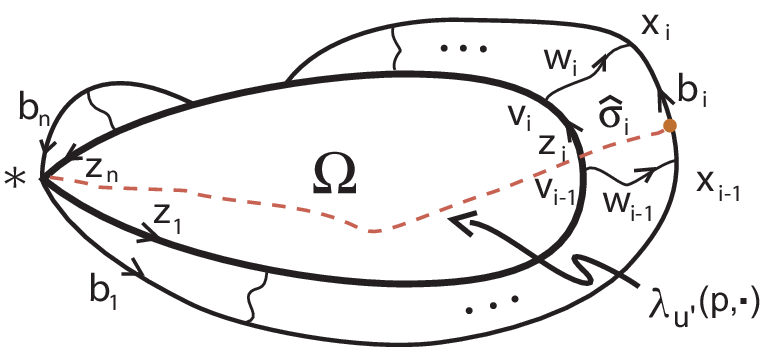
See Figure 7 for a picture of the resulting diagram.

Now the complex $\Lambda_{u^{\prime}}$ is a van Kampen diagram for the original word $u^{\prime}$ , with respect to the presentation ${\mathcal{P}}^{\prime\prime\prime}=\langle B\mid S\cup S^{\prime\prime\prime}\rangle$ of $H$ , where $S^{\prime\prime\prime}$ is the set of all nonempty words in $B^{*}$ of length at most $\zeta^{\prime\prime\prime}:=2k\zeta+(2k)^{2}+2k+1$ that represent $\epsilon_{H}$ . Let $Y^{\prime\prime\prime}$ be the corresponding Cayley complex.

We define a circular 1-combing $\lambda_{u^{\prime}}:C_{l(u^{\prime})}\times[0,1]\rightarrow\Lambda_{u^{\prime}}$ by extending the map $\omega$ on the subcomplex $\Omega$ (from Step II) as follows. First we let the cell complex $C_{l(u^{\prime})}$ be the complex $C_{l(z^{\prime\prime})}$ with each subpath in $C_{l(z^{\prime\prime})}$ mapping to a path $q_{i}$ in ${\partial}\Omega$ replaced by a single edge. From our definitions of $\widetilde{\phi}$ and $\widetilde{\theta}$ , each $q_{i}$ path is labeled by a nonempty word, and so $C_{l(z^{\prime\prime})}$ is a refinement of the cell complex structure $C_{l(u^{\prime})}$ on $S^{1}$ , and we let $\hat{\beta}:C_{l(u^{\prime})}\rightarrow C_{l(z^{\prime\prime})}$ be the identity on the underlying circle. Next define a homotopy $\tilde{\lambda}:C_{l(z^{\prime\prime})}\times[0,1]\rightarrow\Lambda_{u^{\prime}}$ as follows. For each $1\leq i\leq n$ , let $\tilde{v}_{i}$ be the point in $S^{1}$ with $\omega(\tilde{v}_{i},1)=v_{i}$ . Define $\tilde{\lambda}(\tilde{v}_{i},t):=\omega(\tilde{v}_{i},2t)$ for $t\in[0,\frac{1}{2}]$ , and let $\tilde{\lambda}(\tilde{v}_{i},t)$ for $t\in[\frac{1}{2},1]$ be a constant speed path along $p_{i}$ from $v_{i}$ to $x_{i}$ . On the interior of the edge $\tilde{e}_{i}$ from $\tilde{v}_{i-1}$ to $\tilde{v}_{i}$ , define the homotopy $\tilde{\lambda}|_{\tilde{e}_{i}\times[0,\frac{1}{2}]}$ to follow $\omega|_{\tilde{e}_{i}\times[0,1]}$ at double speed, and let $\tilde{\lambda}|_{\tilde{e}_{i}\times[\frac{1}{2},1]}$ go through the 2-cell $\hat{\sigma}_{i}$ (or, if there is no such cell, let this portion of $\tilde{\lambda}$ be constant) from $q_{i}$ to $\check{e}_{i}$ . Finally, we define the circular 1-combing $\lambda_{u^{\prime}}:C_{l(u^{\prime}))}\times[0,1]\rightarrow\Lambda_{u^{\prime}}$ by $\lambda_{u^{\prime}}:=\tilde{\lambda}\circ(\hat{\beta}\times id_{[0,1]})$ . (A path $\lambda_{u^{\prime}}(p,\cdot)$ is illustrated by the dashed path in Figure 7). This map $\lambda_{u^{\prime}}$ is a circular 1-combing for the diagram $\Lambda_{u^{\prime}}$ .

Next we analyze the intrinsic tameness of $\lambda_{u^{\prime}}$ . Since $\Omega$ is a subdiagram of $\Lambda_{u^{\prime}}$ , for any vertex $v$ in $\Omega$ , we have $d_{\Lambda_{u^{\prime}}}(*,v)\leq d_{\Omega}(*,v)$ . Given any edge path $\beta$ in $\Lambda_{u^{\prime}}$ from $*$ to $v$ that is not completely contained in the subdiagram $\Omega$ , the subpaths of $\beta$ lying in the “collar” can be replaced by paths along ${\partial}\Omega$ of length at most a factor of $4k^{2}$ longer. Then $d_{\Omega}(*,v)\leq 4k^{2}d_{\Lambda_{u^{\prime}}}(*,v)$ . Hence for any point $q\in\Omega$ , we have $\widetilde{d}_{\Lambda_{u^{\prime}}}(*,q)\leq\widetilde{d}_{\Omega}(*,q)\leq 4k^{2}\widetilde{d}_{\Lambda_{u^{\prime}}}(*,q)+4k^{2}+1+\zeta^{\prime\prime\prime}$ .

Now suppose that $p$ is any point of $C_{l(u^{\prime})}$ and $0\leq s<t\leq 1$ , and that $\Sigma_{u}$ is $f^{i}$ -tame. Since $n<f^{i}(n)+2$ for all $n\in{\mathbb{N}}[\frac{1}{4}]$ from Remark 4.2, from the definition of $f_{2}$ we also have $n<f_{2}(n)$ for all $n$ . If $t\leq\frac{1}{2}$ , then the path $\lambda_{u^{\prime}}(p,\cdot)$ on $[0,t]$ is a reparametrization of $\omega(p,\cdot)$ , and so Step II, the fact that $f_{2}^{i}$ is nondecreasing, and the inequalities above give

$\displaystyle\widetilde{d}_{\Lambda_{u^{\prime}}}(*,\lambda_{u^{\prime}}(p,s))$	$\displaystyle\leq$	$\displaystyle\widetilde{d}_{\Omega}(*,\lambda_{u^{\prime}}(p,s))$
	$\displaystyle<$	$\displaystyle f_{2}^{i}(\widetilde{d}_{\Omega}(*,\lambda_{u^{\prime}}(p,t)))$
	$\displaystyle\leq$	$\displaystyle f_{2}^{i}(4k^{2}\widetilde{d}_{\Lambda_{u^{\prime}}}(*,\lambda_{u^{\prime}}(p,t))+4k^{2}+1+\zeta^{\prime\prime\prime}).$

If $t>\frac{1}{2}$ and $s\leq\frac{1}{2}$ , then we have $\widetilde{d}_{\Lambda_{u^{\prime}}}(*,\lambda_{u^{\prime}}(p,s))<f_{2}^{i}(4k^{2}\widetilde{d}_{\Lambda_{u^{\prime}}}(*,\lambda_{u^{\prime}}(p,\frac{1}{2}))+4k^{2}+1+\zeta^{\prime\prime\prime})$ and $|\widetilde{d}_{\Lambda_{u^{\prime}}}(*,\lambda_{u^{\prime}}(p,t))-\widetilde{d}_{\Lambda_{u^{\prime}}}(*,\lambda_{u^{\prime}}(p,\frac{1}{2}))|<\zeta^{\prime\prime\prime}+1$ , so

\widetilde{d}_{\Lambda_{u^{\prime}}}(*,\lambda_{u^{\prime}}(p,s))<f_{2}^{i}(4k^{2}(\widetilde{d}_{\Lambda_{u^{\prime}}}(*,\lambda_{u^{\prime}}(p,t))+\zeta^{\prime\prime\prime}+1)+4k^{2}+1+\zeta^{\prime\prime\prime}).

If $s>\frac{1}{2}$ , then

\displaystyle\widetilde{d}_{\Lambda_{u^{\prime}}}(*,\lambda_{u^{\prime}}(p,s))

\displaystyle\leq

\displaystyle\widetilde{d}_{\Lambda_{u^{\prime}}}(*,\lambda_{u^{\prime}}(p,t))+\zeta^{\prime\prime\prime}+1<f_{2}^{i}(\widetilde{d}_{\Lambda_{u^{\prime}}}(*,\lambda_{u^{\prime}}(p,t)))+\zeta^{\prime\prime\prime}+1.

Then $\lambda_{u^{\prime}}$ is $f_{3}^{i}$ -tame for the function $f_{3}^{i}(n):=f_{2}^{i}(4k^{2}n+8k^{2}+1+(4k^{2}+1)\zeta^{\prime\prime\prime})+\zeta^{\prime\prime\prime}+1$ .

We note that we have now completed the proof of Theorem 6.1 in the intrinsic case: The circular 1-combings of the $S^{1}$ -combed filling $\{(\Lambda_{u^{\prime}},\lambda_{u^{\prime}})\mid u^{\prime}\in B^{*},u^{\prime}=_{H}\epsilon_{H}\}$ (over the presentation ${\mathcal{P}}^{\prime\prime\prime}=\langle B\mid S\cup S^{\prime\prime\prime}\rangle$ ) are $f_{3}^{i}$ -tame, and so Proposition 4.3 says that $(H,{\mathcal{P}}^{\prime\prime\prime})$ has an intrinsic tame filling function Lipschitz equivalent to $f_{3}^{i}$ , and hence also to $f^{i}$ .

The analysis of the extrinsic tameness in this step is simplified by the fact that for all $q\in\Omega$ , we have $\widetilde{d}_{Y^{\prime\prime}}(\epsilon_{H},\pi_{\Omega}(q))=\widetilde{d}_{Y^{\prime\prime\prime}}(\epsilon_{H},\pi_{\Lambda_{u^{\prime}}}(q))$ , since the 1-skeleta of $Y^{\prime\prime}$ and $Y^{\prime\prime\prime}$ are determined by the generating sets of the presentations ${\mathcal{P}}^{\prime\prime}$ and ${\mathcal{P}}^{\prime\prime\prime}$ , which are the same. A similar argument to those above shows that if $\pi_{\Delta_{u}}\circ\Sigma_{u}$ is $f^{e}$ -tame, then $\pi_{\Delta_{u^{\prime}}}\circ\lambda_{u^{\prime}}$ is $f_{3}^{e}$ -tame for the function $f_{3}^{e}(n):=f_{2}^{e}(n+\zeta^{\prime\prime\prime}+1)+\zeta+1$ .

Step IV. For $u^{\prime}$ over ${\mathcal{P}}^{\prime}$ : Finally, we turn to building a van Kampen diagram $\Delta_{u^{\prime}}^{\prime}$ for $u^{\prime}$ over the original presentation ${\mathcal{P}}^{\prime}$ . For each nonempty word $w$ over $B$ of length at most $\zeta^{\prime\prime\prime}$ satisfying $w=_{H}\epsilon_{H}$ , let $\Delta_{w}^{\prime}$ be a fixed choice of van Kampen diagram for $w$ with respect to the presentation ${\mathcal{P}}^{\prime}$ of $H$ , and let ${\mathcal{F}}$ be the (finite) collection of these diagrams. A diagram $\Delta_{u^{\prime}}^{\prime}$ over the presentation ${\mathcal{P}}^{\prime}$ is built by replacing 2-cells of $\Lambda_{u^{\prime}}$ , proceeding through the 2-cells of $\Lambda_{u^{\prime}}$ one at a time. Let $\tau$ be a 2-cell of $\Lambda_{u^{\prime}}$ , and let $*_{\tau}$ be a choice of basepoint vertex in ${\partial}\tau$ . Let $x$ be the word labeling the path ${\partial}\tau$ starting at $*_{\tau}$ and reading counterclockwise. Since $l(x)\leq L$ , there is an associated van Kampen diagram $\Delta_{\tau}^{\prime}=\Delta_{x}^{\prime}$ in the collection ${\mathcal{F}}$ . Note that although $\Lambda_{u^{\prime}}$ is a combinatorial 2-complex, and so the cell $\tau$ is a polygon, the boundary label $x$ may not be freely or cyclically reduced. The van Kampen diagram $\Delta_{x}^{\prime}$ may not be a polygon, but instead a collection of polygons connected by edge paths, and possibly with edge path “tendrils”. We replace the 2-cell $\tau$ with a copy $\Delta_{\tau}^{\prime}$ of the van Kampen diagram $\Delta_{x}^{\prime}$ , identifying the boundary edge labels as needed, obtaining another planar diagram. Repeating this for each 2-cell of of the resulting complex at each step, results in the van Kampen diagram $\Delta_{u^{\prime}}^{\prime}$ for $u^{\prime}$ with respect to ${\mathcal{P}}^{\prime}$ .

From the process of constructing $\Delta_{u^{\prime}}^{\prime}$ from $\Lambda$ , for each 2-cell $\tau$ there is a continuous onto map $\tau\rightarrow\Delta_{\tau}^{\prime}$ preserving the boundary edge path labeling, and so there is an induced continuous surjection $\gamma:\Lambda_{u^{\prime}}\rightarrow\Delta_{u^{\prime}}^{\prime}$ . Note that the boundary edge paths of $\Lambda_{u^{\prime}}$ and $\Delta_{u^{\prime}}^{\prime}$ are the same. Then the composition $\Sigma_{u^{\prime}}^{\prime}:=\gamma\circ\lambda_{u^{\prime}}:C_{l(u^{\prime})}\times[0,1]\rightarrow\Delta_{u^{\prime}}^{\prime}$ is a circular 1-combing.

To analyze the extrinsic tameness, we first note that for all points $\hat{q}\in\Lambda_{u^{\prime}}^{(1)}$ , the images $\pi_{\Lambda_{u^{\prime}}}(\hat{q})$ in $Y^{\prime\prime\prime}$ and $\pi_{\Delta_{u^{\prime}}^{\prime}}(\gamma(\hat{q}))$ in $Y$ are the same point in the 1-skeleta $Y^{(1)}=(Y^{\prime\prime\prime})^{(1)}$ , and so $\widetilde{d}_{Y^{\prime\prime\prime}}(\epsilon_{H},\pi_{\Lambda_{u^{\prime}}}(\hat{q}))=\widetilde{d}_{Y}(\pi_{\Delta_{u^{\prime}}^{\prime}}(\gamma(\hat{q})))$ . Let $M:=2\max\{\widetilde{d}_{\Delta}(*,r)\mid\Delta\in{\mathcal{F}},r\in\Delta\}$ .

Suppose that $p$ is any point in $C_{l(u^{\prime})}$ and $0\leq s<t\leq 1$ , and that $\pi_{\Delta_{u}}\circ\Sigma_{u}$ is $f^{e}$ -tame. If $\lambda_{u^{\prime}}(p,s)\in\Lambda_{u^{\prime}}^{(1)}$ , then define $s^{\prime}:=s$ ; otherwise, let $0\leq s^{\prime}<s$ satisfy $\lambda_{u^{\prime}}(p,s^{\prime})\in\Lambda_{u^{\prime}}^{(1)}$ and $\lambda_{u^{\prime}}(p,(s^{\prime},s])$ is a subset of a single open 2-cell of $\Lambda_{u^{\prime}}$ . Similarly, if $\lambda_{u^{\prime}}(p,t)\in\Lambda_{u^{\prime}}^{(1)}$ , then define $t^{\prime}:=t$ , and otherwise, let $t<t^{\prime}\leq 1$ satisfy $\lambda_{u^{\prime}}(p,t^{\prime})\in\Lambda_{u^{\prime}}^{(1)}$ and $\lambda_{u^{\prime}}(p,[t,t^{\prime}))$ is a subset of a single open 2-cell of $\Lambda_{u^{\prime}}$ . From Remark 4.2 and the choice of $f_{3}^{e}$ , we also have $n<f_{3}^{e}(n)$ for all $n\in{\mathbb{N}}[\frac{1}{4}]$ . Then

$\displaystyle\widetilde{d}_{Y}(\epsilon_{H},\pi_{\Delta_{u^{\prime}}^{\prime}}(\Sigma_{u^{\prime}}(p,s)))$	$\displaystyle=$	$\displaystyle\widetilde{d}_{Y}(\epsilon_{H},\pi_{\Delta_{u^{\prime}}^{\prime}}(\gamma(\lambda_{u^{\prime}}(p,s))))$
	$\displaystyle\leq$	$\displaystyle\widetilde{d}_{Y}(\epsilon_{H},\pi_{\Delta_{u^{\prime}}^{\prime}}(\gamma(\lambda_{u^{\prime}}(p,s^{\prime}))))+M$
	$\displaystyle=$	$\displaystyle\widetilde{d}_{Y^{\prime\prime\prime}}(\epsilon_{H},\pi_{\Lambda_{u^{\prime}}}(\lambda_{u^{\prime}}(p,s^{\prime})))+M$
	$\displaystyle<$	$\displaystyle f_{3}^{e}(\widetilde{d}_{Y^{\prime\prime\prime}}(\epsilon_{H},\pi_{\Lambda_{u^{\prime}}}(\lambda_{u^{\prime}}(p,t^{\prime}))))+M$
	$\displaystyle=$	$\displaystyle f_{3}^{e}(\widetilde{d}_{Y}(\epsilon_{H},\pi_{\Delta_{u^{\prime}}^{\prime}}(\gamma(\lambda_{u^{\prime}}(p,t^{\prime})))))+M$
	$\displaystyle\leq$	$\displaystyle f_{3}^{e}(\widetilde{d}_{Y}(\epsilon_{H},\pi_{\Delta_{u^{\prime}}^{\prime}}(\gamma(\lambda_{u^{\prime}}(p,t))))+M)+M.$

Therefore $\pi_{\Delta_{u^{\prime}}^{\prime}}\circ\Sigma_{u^{\prime}}^{\prime}$ is $f_{4}^{e}$ -tame, for the function $f_{4}^{e}(n):=f_{3}^{e}(n+M)+M$ . Since the functions $f_{j}^{e}$ and $f_{j+1}^{e}$ are Lipschitz equivalent for all $j$ , then $f_{4}^{e}$ is Lipschitz equivalent to $f^{e}$ .

Now the collection $\{(\Delta_{u^{\prime}}^{\prime},\Sigma_{u^{\prime}}^{\prime})\mid u^{\prime}\in B^{*},u^{\prime}=_{H}\epsilon_{H}\}$ is a $S^{1}$ -combed filling for the pair $(H,{\mathcal{P}}^{\prime})$ such that each $\pi_{\Delta_{u^{\prime}}^{\prime}}\circ\Sigma_{u^{\prime}}^{\prime}$ is tame with respect to a function that is Lipschitz equivalent to $f^{e}$ , and Proposition 4.3 completes the proof. ∎

The obstruction to applying Step IV of the above proof in the intrinsic case stems from the fact that the map $\gamma:\Lambda_{u^{\prime}}\rightarrow\Delta_{u^{\prime}}^{\prime}$ behaves well with respect to extrinsic coarse distance, but may not behave well with respect to intrinsic coarse distance. The latter results because the replacement of a 2-cell $\tau$ of $\Lambda_{u^{\prime}}$ with a van Kampen diagram $\Delta_{\tau}^{\prime}$ can result in the identification of vertices of $\Lambda_{u^{\prime}}$ .

References

[1] J. Belk and K.-U. Bux, Thompson’s group $F$ is maximally nonconvex, In: Geometric methods in group theory, Contemp. Math. 372, pp. 131-146, Amer. Math. Soc., Providence, RI, 2005.
[2] N. Brady, T. Riley, and H. Short, The geometry of the word problem for finitely generated groups, Advanced Courses in Mathematics, CRM Barcelona, Birkhäuser Verlag, Basel, 2007.
[3] M. Bridson, The geometry of the word problem, In: Invitations to geometry and topology, Oxf. Grad. Texts Math. 7, pp. 29–91, Oxford Univ. Press, Oxford, 2002.
[4] M. Bridson and T. Riley, Extrinsic versus intrinsic diameter for Riemannian filling-discs and van Kampen diagrams, J. Differential Geom. 82 (2009), 115-154.
[5] M. Brittenham and S. Hermiller, A uniform model for almost convexity and rewriting systems, arXiv:1410.2342.
[6] J.W. Cannon, Almost convex groups, Geom. Dedicata 22 (1987), 197–210.
[7] S. Cleary, S. Hermiller, M. Stein and J. Taback, Tame combing and almost convexity conditions, Math. Z. 269 (2011) 879-915.
[8] S. Cleary and J. Taback, Thompson’s group $F$ is not almost convex, J. Algebra 270 (2003), 133149.
[9] S.M. Gersten, Isoperimetric and isodiametric functions of finite presentations, In: Niblo, G.A., Roller, M.A. (eds.) Geometric group theory volume 1. London Math. Soc. Lecture Note Ser. 181, pp. 79–96, Cambridge University Press, Cambridge, 1993.
[10] S.M. Gersten, Dehn functions and $l_{1}$ -norms of finite presentations, In: Algorithms and classification in combinatorial group theory, G. Baumslag, C.F. Miller III, eds., M.S.R.I. Publications 23, pp. 195–224, Berlin Heidelberg New York: Springer, 1992.
[11] V.S. Guba, The Dehn function of Richard Thompson’s group $F$ is quadratic, Invent. Math. 163 (2006), 313342.
[12] S. Hermiller and J. Meier, Measuring the tameness of almost convex groups, Trans. Amer. Math. Soc. 353 (2001), 943-962.
[13] R.C. Lyndon and P.E. Schupp, Combinatorial group theory, Classics in Mathematics, Springer-Verlag, Berlin, 2001.
[14] M.L. Mihalik and S.T. Tschantz, Tame combings of groups, Trans. Amer. Math. Soc. 349 (1997), 4251–4264.
[15] C. Thiel, Zur Fast-Konvexität einiger nilpotenter Gruppen, Bonner Mathematische Schriften, 1992.
[16] Thompson’s group at 40 years: Preliminary problem list, AIM Research Conference Center, January 2004, available from
http://www.aimath.org/WWN/thompsonsgroup/thompsonsgroup.pdf.
[17] S.T. Tschantz, private communication.