On the Convexity of Image of a
Multidimensional Quadratic Map
Anatoly Dymarsky
Skolkovo Institute of Science and Technology,
Skolkovo Innovation Center, Nobel st. 3, Moscow, Russia, 143026
Department of Physics and Astronomy, University of Kentucky,
Lexington, KY 40506
Abstract
We study convexity of image of a general multidimensional quadratic map. We split the full image into two parts by an appropriate hyperplane such that one part is compact, and formulate a sufficient condition for convexity of the compact part. We propose a way to identify such convex parts of the full image which can be used in practical applications. By shifting the hyperplane to infinity we extend the sufficient condition for convexity to apply to the full image of the quadratic map. As a related result, we formulate a novel condition for the joint numerical range of -tuple of hermitian matrices to be convex. Finally, we illustrate our findings by considering several examples. In particular we prove convexity of solvability set for the Power Flow equations in case of DC networks.
Keywords: convexity, quadratic transformation, multidimensional quadratic mapping, vector-valued quadratic forms, joint numerical range, Polyak convexity principle, Power Flow equations
1 Introduction and Main Results
In this paper we consider a multidimensional quadratic map of general form (or ) defined by an -tuple of symmetric (hermitian) matrices , an -tuple of vectors (or ), and a vector ,11 1 Symbol ∗ stands for transposition or hermitian conjugation depending on the context.
| (1.1) |
An important question arising in many applications is when the image of the quadratic map (1.1),
| (1.2) |
is convex. This question was previously studied in case of small or when only a few of ’s are linearly independent, see [1, 2, 3] and [4] for references and a brief historic overview. Identifying necessary and sufficient conditions for the convexity of (1.2) for general remains an open problem which we investigate in this paper.
Although the results concerning convexity of as a whole are scarce, something can be said about convexity of the image of locally. In particular, for any non-linear map there is an upper bound on the size of a ball such that its image is convex [5]. Because of a very broad scope of this result the corresponding bound on is always finite and can never fully cover . The bound of [5] was improved in [6] for the case of a general quadratic map (1.1) and an ellipsoid-shaped ball defined through some positive-definite matrix , ,
| (1.3) | |||
| (1.4) |
Above we introduced to denote the smallest generalized eigenvalue of with respect to .22 2 The smallest generalized eigenvalue can be defines as . In (1.3) and in what follows a sum of a matrix and a number understood in a sense that the number is multiplied by the identity matrix of an appropriate size. The dot product stands for the standard scalar product in the Euclidean space. Also notice the appearance of the “plus” norm in (1.3).
Reference [6] proves that is strictly convex for . Now, if for any non sign-definite combination , , the projection of the vector on the eigenspace corresponding to the smallest generalized eigenvalue of is non-vanishing, is infinite and the image is strictly convex for any . Consequently we have the following proposition.
Proposition 1. If for any point and any the value of is infinite
the full image is convex. This is a novel sufficient condition for the convexity of image of a general multidimensional quadratic map.
The proof is trivial. For any two points we consider their pre-images (any pre-images if there are many). For a significantly large , and consequently all points for lie within .
What happens if is very large but not infinite? Strictly speaking there is not much we can say about convexity of in this case. It is reasonable to expect that might still be very close to be convex because the image of a very large ball is convex. Unfortunately some points might be mapped in finite distance away from the origin for any, even infinitely large and this could spoil convexity of the full image. If somehow we could arrange for , , to be large with some appropriate norm when is large than not only would be convex when is infinite, but also we could outline a compact part of (an intersection of with a “ball” of a certain size defined by the norm ), which is convex when is finite. This idea, which we develop in section 2, leads to the following result.
For any vector such that the combination is positive-definite, , let us define the point . This is the unique point where the supporting hyperplane orthogonal to “touches” . Let us introduce the following limit
| (1.5) | |||
| (1.6) |
Proposition 2. The compact set is convex. If is infinite the whole image is convex.
The Proposition 2 is reformulated in section 4 in a more application-friendly way. See Proposition 2’ and Comment 4 there.
Comment 1. The convex set can be defined as a compact part of lying in a half-space defined by a certain hyperplane , where for any the corresponding orthogonal hyperplane is defined as
| (1.7) |
The hyperplane is the supporting hyperplane of perpendicular to . Hence is the part of bounded by two parallel hyperplanes separated by the distance apart. This is illustrated in Fig. 1.
Comment 2. The two criteria for convexity (Proposition 1 and Proposition 2) are complimentary to each other in the following sense. In (1.3) is a regular point of and thus may vanish. On the contrary in (1.5) belongs to the boundary .
Comment 3. The sufficient condition of Proposition 1 depends on the choice of . Potentially, if is infinite for some it might be finite for some other . On the contrary if (1.5) is infinite for some (and corresponding ), it will be infinite for all other choices of as well. If is finite its value depends on .
This is explained in section 2.1.


We derive the expression for (1.5) and prove Proposition 2 in section 2, while Proposition 1 directly follows from the results of [6]. In section 3 we discuss how our results pertaining to convexity of can be related to the classical question of convexity of the joint numerical range of -tuple of symmetric (hermitian) matrices. In particular we formulate novel sufficient conditions for convexity of the joint numerical range in the subsection 3.1. In section 4 we reformulate Proposition 2 and discuss different ways of calculating . In particular we outline an easy-to-calculate conservative bound on in the subsection 4.1. In this way we formulate a practical way to outline a convex part of , which can be used in applications. Section 5 is devoted to applications and examples. First, we prove convexity of solvability set for the Power Flow equations for the DC networks. Then we illustrate main points of this paper in case of several concrete examples. In one case we consider an example when the image is not convex and calculate both exactly and approximately, using the bound of the subsection 4.1.
2 Convexity of
Let us first approach the question of convexity of locally. From now on we assume that the -tuple of matrices is definite in the sense of reference [8], i.e. there is a positive-definite combination for some . The corresponding supporting hyperplane touches only at one point ,
| (2.1) |
This is schematically depicted in Fig. 1. Provided the boundary of is smooth and strongly convex at it is tempting to say that the compact part of lying in a half-space defined by the hyperplane , would be convex, at least for very small . It is easy to see that the compact part of bounded by , is the image of the ball under the map . We would like to find an upper bound on such that the image is convex. This problem almost identically repeats the question studied by Polyak [5] for general , and further investigated in [6] in case of quadratic , with one crucial distinction: point is not a regular point of .
The following observation drastically simplifies further analysis: each ellipsoid is mapped into its own hyperplane . Hence the convexity of requires convexity of for all . Up to a translation and a trivial change of basis in the image is nothing but the inhomogeneous joint numerical range, the notion we introduced in [6],
| (2.2) |
for an -tuple of symmetric (hermitian) matrices and a -tuple of vectors . There it was proven that if
| (2.3) |
is strictly convex (strongly convex for strong inequality in (2.3)) and smooth. In fact (2.3) is a criterion for stable convexity, i.e. impossibility to ruin convexity of by an infinitesimal deformation of .
Applying this directly to the image will fail because the latter is “flat”, i.e. it lies within the hyperplane and hence can not be strictly convex. This is easy to fix by considering an orthogonal projection of on . Now the criterion (2.3) can be applied directly to the -dimensional inhomogeneous joint numerical range ,
| (2.4) |
The minimum (2.4) is taken over the space of the equivalence classes . Since the minimized expression is homogeneous in the condition could be substituted by . (Notice, that if , (2.4) vanishes.)
Clearly, convexity of for all is a necessary condition for the convexity of but may not be sufficient. To establish convexity of let us choose an arbitrary vector and find an intersection of with a supporting hyperplane orthogonal to which touches “from below”,
| (2.5) |
For collinear with the answer is simple. When , , the hyperplane intersects at the unique point . When the intersection is a -dimensional convex set . For not collinear with we can first find a conditional minimum for and then minimize with respect to in the interval . This problem was solved in [6] where it was shown that the minimum is achieved at such that , uniquely determined by the conditions
| (2.6) |
is equal to . Since is a monotonically increasing function of on the interval such a point is unique. Correspondingly the supporting hyperplane intersects at a unique point. Hence where stands for convex hull. Now, to prove that is convex we need to show that any point of belongs to . This is obviously true because an intersection of with the hyperplane for any is either empty or convex. This finishes the proof of Proposition 2.
2.1 Geometrical meaning of
To interpret geometrically we would need to understand different scenarios of how may intersect with its supporting hyperplanes. Let us consider a vector and find a supporting hyperplane to that is orthogonal to . There are several possible scenarios. First, is sign-definite. The corresponding supporting hyperplane intersects at the unique point . Second, has both positive and negative eigenvalues. There is no corresponding supporting hyperplane in this case because stretches to infinity in both directions along . Finally, is semi-definite and degenerate. There are two possibilities (Fredholm alternative) in this case. If the equation admits no solution, there is no supporting hyperplane to orthogonal to because stretches to infinity in both directions along . Another option is when there is a whole linear space of solutions of . Each such solution corresponds to a point from the boundary belonging to the same supporting hyperplane orthogonal to .
In case a supporting hyperplane intersects over more than one point we would like to call all points of belonging to this supporting hyperplane a ‘‘flat edge’’.33 3 More precisely we should define “flat edge” as an intersection of with a supporting hyperplane if the pre-image of this intersection consists of more than one point. But a “flat edge” defined this way can consist of one point only if all matrices have a common zero eigenvector which is in contradiction with the assumption that the set of ’s is definite. If includes “flat edges”, can not be strictly convex and certainly can not be stably convex. In general such will not be convex at all.
Now let us look at the definition of (1.5). For any , , the limit in (1.5) will be finite only if the equation
| (2.7) |
has nontrivial solution(s). Since is degenerate and positive semi-definite, existence of nontrivial solutions is the same as the existence of a “flat edge” orthogonal to . Hence will be infinite unless there is a supporting hyperplane touching at more than one point. The latter is the property of and and does not depend on the choice of and .
It is easy to show that for any vector such that is orthogonal to a “flat edge” (namely, but and the space of solutions is non-trivial), the limit in (1.5) calculates the minimum value of . Consequently is the distance from the supporting hyperplane orthogonal to to a closest point belonging to any “flat edge” inside . This is depicted in Fig. 2.1. This also explains that is stably convex for and is not stably convex .
A comment is in order. If were compact, absence of “flat edges” would immediately guarantee that the outer boundary is a boundary of the convex hull of while the latter is strictly convex. But in a non-compact case this is not true. Fig. 2b provides a non-compact example without “flat edges” (meaning that each supporting hyperplane is touching the figure is exactly at one point) when the outer boundary is not the boundary of the convex hull. Hence the proof that the absence of “flat edges” () implies that the boundary confines a convex set, which was presented in section 2, was not superfluous.

3 Connection with the joint numerical range
In this section we would like to look at the convexity of from a slightly different angle. Shifting by a constant does not affect convexity and therefore without loss of generality we assume . Then can be thought of as an intersection of the image of the “extended” homogeneous quadratic map (or ) and a hyperplane
| (3.1) |
where is the -th basis vector and
| (3.2) | |||
| (3.8) |
Obviously, convexity of would imply convexity of . Validity of the converse statement is a subject of the following discussion. On general grounds convexity of together with the conic structure of and the relation (3.1) do not imply convexity of but only of .
Possible advantage of introducing is that convexity of homogeneous quadratic maps was studied previously in [8]. There is a general relation between definite homogeneous quadratic maps and joint numerical ranges of some auxiliary matrices. Geometrically is a cone. If is definite, i.e. there is a linear combination , the base of the cone , is compact and equal (up to a linear isomorphism) to a joint numerical range of matrices which can be explicitly constructed from . Hence proving convexity of is the same as establishing convexity of . The latter is a question with a long and rich history.
For an -tuple of symmetric or hermitian matrices the joint numerical range is defined as follows
| (3.9) |
where are symmetric or Hermitian matrices and or correspondingly. The question of convexity of goes back to Housdorff and Toeplitz [9] who proved that is always convex for hermitian matrices (i.e. ) and . There are numerous results for small [10, 11, 12, 13] (also see [14] for references) and a few specific conditions rendering non-convex. The case of general is not fully understood, although there is a sufficient condition that guarantees that is strongly convex and smooth: if for all linear combinations of the dimension of the eigenspace corresponding to the lowest eigenvalue is the same [7]. In terms of the corresponding map this is the condition that for any linear combination such that , but , dimension of is the same. This condition is a generalization of roundness defined in [8] which guarantees “roundness” (strict convexity and smoothness) of the base of the cone .
We will see later that in our case of interest (3) the condition that remains the same for different is not satisfied. Thus the results of [7], [8] do not help to establish convexity of . In the following we will reverse the logic and extend the sufficient condition for convexity of , Proposition 2, to and . In this way we formulate new criteria for the convexity of the joint numerical range.
From now on we assume that given by (1.5) is infinite, which implicitly assumes the set of ’s is definite. Let us show that the set of ’s given by (3) is definite as well. Starting from an appropriate , let us consider the vector ,
| (3.10) |
Then the matrix is positive-definite as follows from the Sylvester’s criterion.
Infinite value of implies that for any , , equation has no solution (see section 2.1). This immediately implies that any , where is either trivial or must satisfy , unless . Hence for all appropriate , except for the special case when . Presence of this exceptional direction makes it impossible to apply the results of [7, 8]. Indeed those works were focused on strictly convex and smooth joined numerical range , properties guaranteed by constancy of for all appropriate such that , but . On the contrary, in our case has a “flat edge” perpendicular to the direction of (after projection on ), which is a direct consequence of for one particular direction . The joint numerical range of this kind – with one side being flat (flat edge) – is shown in Fig. 3.

The “flat edge” of is an -dimensional figure. Let us first establish it is convex. We introduce
| (3.11) |
and notice that is isomorphic to the “flat edge” of . For any , is isomorphic to where corresponding (and hence ) is related to through (3.10) and is some function of an other parameters. The limit corresponds to . For any sufficiently small , where , we proved that is strongly convex. Hence by continuity is convex as well.
The rest of the proof closely follows the logic outlined in section 2. Let us consider a vector , , , and find an intersection of with the supporting hyperplane orthogonal to touching “from below”
| (3.12) |
For any the intersection consists of a unique point except for when it is a convex “flat edge”. Hence the boundary is the boundary of the convex hull of , . Finally, since the intersection is convex (or empty) for any we conclude that all points confined by belong to . This establishes convexity of and provided the criterion for convexity of , Proposition 2, is satisfied.
3.1 New Criteria for Convexity for the Joint Numerical Range
The proof of convexity of can be cast in a form of a self-contained criterion for convexity based only on the properties of matrices .
Let us consider a joint numerical range (3.9) defined by an -tuple of symmetric (hermitian) matrices . If for any linear combination , its smallest eigenvalue is not degenerate, is convex [7]. If for any linear combination , , where is a fixed vector, its smallest eigenvalue is not degenerate, but the smallest eigenvalue of is -times degenerate, is convex if the following condition is satisfied. We add the identity matrix to the set of ’s thus bringing the total number of matrices to . By changing a basis in we bring to the form of from (3). By taking a linear combination of with other matrices we bring them to the form of from (3) and in this way define vectors and matrices . Now, if the auxiliary map defined by through (1.1) satisfies the convexity criterion of Proposition 2, , then is convex. This is the first new sufficient condition for convexity.
In fact there is another sufficient criterion of convexity of “buried” inside the proof in section 3. Indeed, the “flat edge” is the joint numerical range associated with the homogeneous quadratic map . Hence the second new sufficient condition for the convexity of the joint numerical range can be formulated as follows. Let us consider a joint numerical range (3.9) defined by an -tuple of symmetric (hermitian) matrices . By adding the identity matrix to the set of ’s we define an -tuple of matrices . If for any -tuple of vectors the corresponding quadratic map
| (3.13) |
satisfies the convexity criterion of Proposition 2, , then is convex.
The two new sufficient conditions for convexity formulated above invoke auxiliary map . We leave the task of formulating these criteria for convexity of free of any reference to and for the future.
4 Different Approaches to Calculating
In section 2 we proved that a compact part of lying in a half-space defined by the hyperplane is compact. To make this a practical method of carving a compact subregion within suitable for applications we would need to be able to determine for a given . A straightforward approach would be to use the definition (1.5). We prefer to rewrite as , where is given by (2.7). Notice that matrices for all , exhaust all positive-semidefinite combinations of with a non-trivial kernel. Hence vectors orthogonal to is enough to parametrize the entire boundary of the convex cone of the positive-semidefinite linear combinations of . Furthermore and therefore minimization problem (1.5) can be naturally defined on the boundary ,
| (4.1) | |||
| (4.2) |
Unfortunately this problem is not convex. A naive extension of this problem to the interior of is not a viable option because , even when . We conclude that the minimization problem (1.5) can not be immediately reduced to a convex optimization problem admitting an efficient solution.
This motivates us to approach the problem of calculating from a slightly different angle. As was discussed in section 2.1 the expression minimized in (4.1) is finite in the limit only when for some vector such that and , i.e. is degenerate, the following equation has a solution, . The latter is trivially equivalent to solvability of . Let us define the set of all such vectors ,
| (4.3) |
Because of the additional constraints, in real case is a -dimensional sub-manifold of -dimensional . (In complex case is -dimensional.) In principle can be calculated by minimizing
| (4.4) |
over ,
| (4.5) |
In (4.4) denotes pseudo-inverse. This leads to the following application -friendly reformulation of Proposition 2.
Proposition 2’. The compact subset of the image of the quadratic map (1.2),
| (4.6) |
with defined in (4.5, 4.4),
is convex. (See (2.1) for the definition of .) If is infinite the whole image is convex.
Comment 4. The sufficient condition for convexity can be concisely formulated as follows: if the set is empty, the image is convex.
When the matrix is degenerate, the solvability of is equivalent to for all satisfying . Hence, if (i) a quadratic map (1.1) is definite, i.e. there is such that and (ii) for any vector , such that is positive semi-definite and degenerate, there is a vector satisfying and , then the image of is convex.
When the set is non-empty and the map is definite, the image is not strictly convex and in a general case it is non-convex at all. In this case one potential strategy to calculate would be to minimize (4.5) numerically, e.g. via gradient descent along .
4.1 Conservative Estimate of
Calculating exactly could be a difficult. Nevertheless for many practical application it would be enough to have an easy-to-calculate conservative estimate . A very similar problem of estimating (1.3) was addressed in [6] and here we employ the same strategy. The first step is the inequality
| (4.7) | |||
| (4.8) |
where , and is defined through . Because (4.7) is homogeneous in the condition can be substituted by for some which is positive-definite on the orthogonal compliment to within . Let’s choose which satisfies this requirement (obviously is non-negative; if it develops a zero eigenvalue on the orthogonal compliment to , then, alas, would be zero anyway). It is convenient to diagonalize and bring it to the standard form with the help of some non-degenerate real-valued matrix . Now we can define and since we introduce a new -dimensional vector with the components ,
| (4.9) |
Furthermore using the inequality we arrive at the following approximate conservative estimate of ,
| (4.10) |
Next step would be to calculate or estimate the Lipschitz constant , the problem which was previously addressed in [6].
In fact the estimate (4.10) can be improved if we notice that is invariant under the shifts of by the identity matrix . Hence the better estimate for would be
| (4.11) |
where the minimum is taken over the space of functions satisfying . Obviously we can restrict the class of functions by paying the price of somewhat deteriorating the quality of the estimate. For example could be chosen to be a linear function defined by a vector . Depending on the chosen method to estimate we can either find a minimum with respect to analytically or leave it to numerical analysis.
In case minimization with respect to is difficult, one guideline to choose could be the following. The inequality is saturated when and therefore it makes sense to choose such that any combination has both positive and negative eigenvalues. For example this can be done with help of , which is an optimal condition for .
5 Examples and Applications
5.1 Convexity of solvability set of Power Flow equations for DC networks
The Power Flow equations for DC networks is a set of quadratic equations which express power injections on each bus of the network in terms of real-valued voltages. For a system consisting of buses, , the equations take the following form
| (5.1) |
where is a symmetric admittance matrix of resistances which is defined for each network as follows
Here we adopt the notation to indicated that nodes (buses) and are connected by a line, and in (5.1) we assume that each line is purely resistive, , for any . In what follows we will also assume the network is connected i.e. any two nodes can be connected by a combination of lines.
We choose to be the slack bus, which means . Then the Power Flow equations should be understood as equations expressing powers for , in terms of voltages , where . Hence the Power Flow equations for DC networks define a quadratic map. The solvability set of Power Flow equations is the combination of all feasible powers such that equations (5.1) admit a solution, i.e. it is the image of this quadratic map.
In what follows we prove that solvability set of Power Flow equations (5.1) is convex. This result is closely related to the proof that convex relaxation for Optimal Power Flow problem for DC networks is exact [15]. At the same time convexity of solvability set is a new result which was not covered in literature previously.
The quadratic map defined by (5.1) can be represented in the conventional form (1.1) with , , while , and are given by
| (5.6) |
To verify that the set of matrices is definite it is enough to calculate the sum
| (5.7) |
which is manifestly positive-definite. From the physics point of view, definiteness of map (5.6) is a consequence of the network being resistive, hence the total power dissipated by the lines (first term in (5.7)) is non-negative. From here we immediately conclude that vector in (2.1) can be chosen to be
| (5.8) |
Next we would like to identify the set (4.3). We assume that vector which in particular means that matrix is positive semi-definite and degenerate,
Since all diagonal elements of have to be non-negative and since all we find that all . In fact all must be strictly positive. Indeed, let us assume that for a particular . For to be positive semi-definite all elements must be zero, . This is only possible if for all . And since the network is connected, repeating this consideration enough times, we find for all . This contradicts the assumption , and therefore all .
By definition of matrix must be singular, i.e. there is a normalized vector such that . This vector minimizes the following quadratic form
| (5.13) |
subject to . Taking into account that for any the combination , for the given values of , the quadratic form (5.13) will be minimal if . Hence all components of minimizing (5.13) must have the same sign. Without loss of generality we can assume that . In fact it is possible to show that all minimizing (5.13) must be strictly positive (or negative). To prove that, we assume the opposite, that for some . Then we analyze the equation , namely look at the -the component of vector ,
| (5.14) |
Since all are non-negative and by assumption this equation can be satisfied only if at all nodes connected with . Since the network is connected, by repeating this logic, we find that all components of vector minimizing (5.13) are zero, which contradicts the assumption .
Finally, we consider if the equation can have a solution. The necessary and sufficient condition for the solution to exist is
| (5.15) |
for all vectors satisfying . The equation (5.15) written in terms of has the form
| (5.16) |
Clearly it can not be satisfied because it is a sum of strictly positive terms. We therefore conclude that is empty, hence is infinite and according to Proposition 2’ the solvability set is convex.
5.2 3-bus example
To illustrate some of the ideas discussed above, let us consider a simple network consisting of buses all connected to each other. The corresponding admittance matrix and the quadratic map is given by
| (5.21) | |||||
| (5.22) |
We have established in section 5.1 that the image of the quadratic map , , with being a constant is convex. In section 3 we establish that the convexity of implies convexity of image of the homogeneous quadratic map defined through (3.1). This simply means the functions (5.21,5.22) are amended by
| (5.23) |
and are the functions of all three variables . The associated matrices are as follows
The sum is positive-definite. To find matrices and the joint numerical range associated with the base of the cone we consider two linear combinations of which are linearly independent with ,
| (5.34) |
Upon changing the coordinates in the space of we can bring to be the identity matrix. In these coordinates matrices , , (5.34) are given in the caption of Fig. 3. The convexity of the corresponding joint numerical range depicted in Fig. 3 is thus guaranteed by the first sufficient condition for convexity formulated in section 3.1. It should be noted for completeness that since in this case is only -dimensional, its convexity is also guaranteed by the result of [11].
5.3 4-bus example
Our next example is a -bus network with the admittance matrix
The corresponding expressions (5.1) define the initial quadratic map . The latter gives rise to the homogeneous quadratic map (3.1) with matrices , , given by
We choose , one can check , and define , , through the following linear combinations
| (5.58) |
The joint numerical range is thus the base of the cone . In the coordinates where matrix is the identity matrix, matrices have the following form
According to the first sufficient condition for convexity formulated in section 3.1, the joint numerical range is convex. We would like to emphasize that this is a new result as the convexity of such joint numerical range could not have been established using previously known criteria.


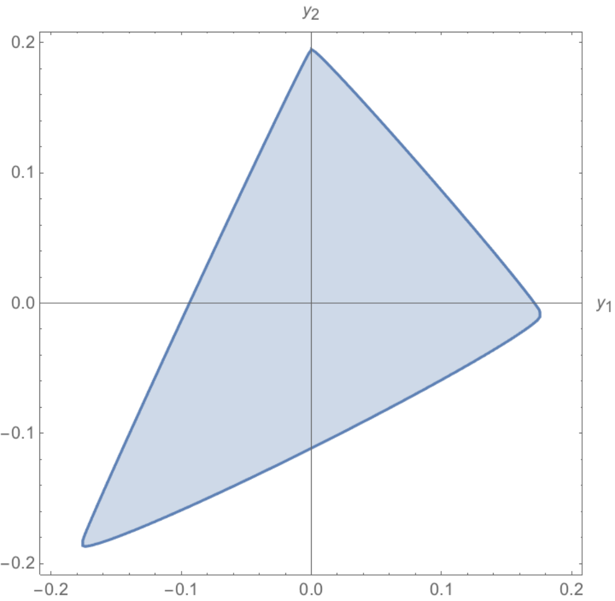
The corresponding joint numerical range , , , is shown in Fig. 4. The “bottom” of that figure, namely the intersection of the image of with the hyperplane , is a flat two-dimensional convex set which is shown in Fig. 5.
Convexity of the latter can be independently deduced from the second new sufficient condition for convexity formulated in section 3.1. Namely, one can start with the expression for powers (5.1) specified by the admittance matrix (5.3). Assuming , powers , , become quadratic homogeneous functions of , . The corresponding matrices are given by the upper left sub-matrices of the matrices (5.3),
while and . This homogeneous quadratic map is definite, . By performing a linear change of variables we can bring to be the identity matrix, while two linearly independent combinations and will be given by (compare with (5.3)),
The convex image of , , is shown in Fig. 5.
5.4 example
Consider a quadratic map with being Pauli matrices
and given by
Clearly, this map is definite. We choose which results in and . Now we identify all vectors such that and degenerate. First, requires , then also specifies . Up to an overall rescaling we parametrize all such vectors by points on ,
| (5.109) |
A normalized vector satisfying is given by
The equation yields
| (5.113) |
with the only solution . Hence consists of only one vector . It is straightforward to calculate using the definition (4.4). Since consists of only one vector .
Let us consider the image of where is a solution of and is an arbitrary complex number. Points belong to the “flat edge” which is an intersection of with the supporting hyperplane orthogonal to . We can find these points explicitly
| (5.114) |
As expected these point lie on a hyperplane . Thus (5.114) defines a map from into with being a quadratic function of and . Quite clearly the image of this map (a parabolic surface in embedded into ) is not convex.
We conclude that the image of specified by (5.4,5.4) is not convex overall, but the compact part defined by the inequality is convex. This is shown in Fig. 6, where we plot the intersection of with the hyperplanes for different values of .


Finally, let us estimate using the approximate approach of section 4.1. In our case is an identity matrix and are given by
Hence matrix is
After introducing
such that we calculate matrices for . To make the presentation concise we do not write the explicit expressions for here. It is important to note that since for were traceless, so will be and . Hence and it can be calculated explicitly
| (5.134) |
Using the constraint (5.134) can be expressed as a function of two independent variables with the maximum corresponding to and ,
| (5.135) |
and according to (4.10) we find
| (5.136) |
Hence, our estimate assures convexity of approximately of the maximal convex subset within .
Acknowledgments
I would like to thank Vasily Pestun and Konstantin Turitsyn for useful discussions.
References
- [1] B. T. Polyak, “Convexity of quadratic transformations and its use in control and optimization,” Journal of Optimization Theory and Applications, 99, 553-583 (1998).
- [2] A. Beck, “On the convexity of a class of quadratic mappings and its application to the problem of finding the smallest ball enclosing a given intersection of balls,” Journal of Global Optimization, Vol. 39, Issue 1, September 2007, p. 113 - 126.
- [3] Y. Xia, “On Local Convexity of Quadratic Transformations,” Journal of the Operations Research Society of China, 2014 Sep 1;2(3):341-50, [arXiv:1405.6042].
- [4] I. Plik, T. Terlaky, “A Servey of S-lemma,” SIAM review, 49(3), 371-418 (2007).
- [5]
B. T. Polyak, “Convexity of Nonlinear Image of a Small Ball with Applications to Optimization,” Set-Valued Analysis, 9(1/2), 159-168 (2001).
B. T. Polyak, “Local Programming,” Comp. Math. and Math. Phys., 41(9), 1259-1266 (2001).
B. T. Polyak, “The convexity principle and its applications,” Bull.Braz.Math.Soc. (N.S.), 34(1), 59-75 (2003). - [6] A. Dymarsky, “Convexity of a Small Ball Under Quadratic Map,” Linear Algebra and its Appl. 488 (20016), pp.109-123, [arXiv:1410.1553].
- [7] E. Gutkin, E. A. Jonckheere, M. Karow, “Convexity of the joint numerical range: topological and differential geometric viewpoints,” Linear Algebra Appl. 376 (2004), 143–171.
- [8] J. Sheriff, “The Convexity of Quadratic Maps and the Controllability of Coupled Systems,” Ph.D. thesis, Harvard University, 2013, UMI publication number 3567063.
- [9]
O. Toepliz, “Das algebraische Analogon zu einem Satze von Fejr,” Mathematische Zeitschrift, 1918, Vol. 2, Issue 1-2, pp. 187-197.
F. Hausdorff, “Der Wertevorrat einer Bilinearform,” Mathematische Zeitschrift, 1919, Vol. 3, pp. 314-316. - [10] L. L. Dines, “On the mapping of quadratic forms,” Bulletin of the AMS, 47, 494-498 (1941).
- [11] L. Brickman, “On the field of values of a matrix,” Proceedings of the AMS, 12, 61-66 (1961).
- [12] A. Barvinok, “A course in Convexity,” Graduate Studies in Mathematics, V. 54, American Mathematical Society, Providence, Rhode Island, 2002.
- [13] F. Bullo, J. Cortes, A. D. Lewis, S. Martinez, “Vector-valued Quadratic Forms in Control Theory,” In V. Blondel and A. Megretski, Unsolved Problems in Mathematical Systems and Control Theory, pages 315-320. Princeton Univesity Press, Princeton, NJ, 2004.
- [14] Y. T. Poon, “Generalized numerical ranges, joint positive definiteness and multiple eigenvalues,” Proc. Amer. Math. Soc., 1997, Vol. 125, N. 6, pp. 1625-1634.
- [15] J. Lavaei, and S. H. Low, “Zero duality gap in optimal power flow problem,” IEEE Transactions on Power Systems, 27(1) (2012), pp.92-107.