Minimum Forcing Sets for Miura Folding Patterns
Abstract
We introduce the study of forcing sets in mathematical origami. The origami material folds flat along straight line segments called creases, each of which is assigned a folding direction of mountain or valley. A subset of creases is forcing if the global folding mountain/valley assignment can be deduced from its restriction to . In this paper we focus on one particular class of foldable patterns called Miura-ori, which divide the plane into congruent parallelograms using horizontal lines and zig-zag vertical lines. We develop efficient algorithms for constructing a minimum forcing set of a Miura-ori map, and for deciding whether a given set of creases is forcing or not. We also provide tight bounds on the size of a forcing set, establishing that the standard mountain-valley assignment for the Miura-ori is the one that requires the most creases in its forcing sets. Additionally, given a partial mountain/valley assignment to a subset of creases of a Miura-ori map, we determine whether the assignment domain can be extended to a locally flat-foldable pattern on all the creases. At the heart of our results is a novel correspondence between flat-foldable Miura-ori maps and -colorings of grid graphs.
1 Introduction
In the mathematical modeling of programmable matter, the topic of self-folding origami—where a pre-programmed material folds itself from an initially flat state in response to some stimulus or mechanism—has been gaining in popularity. The origami material can be pre-programmed to fold along straight lines, called creases, by means of rotation to achieve a mountain or valley fold (for examples, see [6, 9, 10, 12]). In such cases, the self-folding process can be economized by programming only a subset of the creases to self-fold, which would then force the other, passive creases to fold as originally intended. We call such a subset of the creases a forcing set.
Because of the cost of programming creases, finding a forcing set of smallest size in a given crease pattern would be a useful tool for self-folding. To our knowledge, this is the first paper to address this problem in two dimensions.11 1 For one dimensional crease patterns, there are some unpublished forcing set results by a subset of the authors here. Due both to the high computational complexity of dealing with unrestricted crease patterns [3], and to the versatility of modular repeating crease patterns in the design of self-folding shapes [1], our focus here is on finding forcing sets for flat-foldable origami whose folded shape lies flat in the plane, using a restricted set of folds based on the Miura-ori pattern (see Figure 1a). This is a common crease pattern in origami that has found applications ranging from tourist maps to solar panel arrays for satellites [8].
In this paper, we develop efficient algorithms for determining a minimum forcing set of a Miura-ori map, and for deciding whether a given set of creases is forcing or not. Given a partial mountain/valley assignment to a subset of creases of a Miura-ori map, we also determine whether the assignment domain can be extended to cover all creases such that the resulting pattern is locally flat-foldable. Additionally, we show that, for a Miura-ori crease pattern with cells and a flat-foldable assignment of mountain/valley folds to its creases, a forcing set includes at least creases and at most creases. We establish a lower bound of on the size of a forcing set for the standard Miura-ori mountain-valley assignment (described in subsection 1.1), so from this perspective the standard Miura-ori is the “worst” Miura. These results make use of previous work characterizing when a crease pattern at a node is locally flat-foldable [7] (detailed in Section 2) and a novel correspondence between flat-foldable Miura-ori maps and -colorings of grid graphs recently developed in [5] (detailed in Section 3).
Although we are the first to consider the minimum forcing set problem, there is much related work on flat-foldable origami. Arkin et al. [2] give a linear time algorithm for determining if a one dimensional crease pattern is flat-foldable. In [3], Bern and Hayes show how to determine in linear time whether a general crease pattern has a mountain-valley assignment for which every node is locally flat-foldable. This is necessary but not sufficient to ensure that the entire crease pattern is flat-foldable. Deciding whether a crease pattern is flat-foldable is NP-hard [3]. For crease patterns consisting of a regular grid of squares, the complexity of deciding whether a given mountain-valley assignment can be folded flat (the map folding problem) remains open [4], although recent progress has been made on grids [14] and on testing for valid linear orderings of the faces in a flat-folding [15]. In [7], Hull gives upper and lower bounds on the number of flat-foldable mountain-valley assignments on a single-node crease pattern.
1.1 Definitions
A crease pattern is a finite planar straight-line graph drawn on a piece of paper, with edges corresponding to line segments of the crease pattern, and nodes connecting two or more edges. For clarity, we will refer to the edges of the planar graph simply as creases. A crease pattern is flat-foldable if it is the crease pattern of some flat origami; that is, if there is a way of folding the paper so that the folds lie along the creases and the folded shape again lies flat in a plane [3].
For a given crease pattern , let denote the set of creases of the corresponding planar graph. A mountain-valley assignment on , or MV assignment for short, is a function , where indicates a valley crease and indicates a mountain crease. An MV assignment restricts the way a crease pattern folds into some flat origami. Intuitively, if the origami is unfolded back to a piece of paper with one side up and one side down, a mountain fold points up and a valley fold points down. Given a foldable MV assignment , a flat folding that conforms to is not necessarily uniquely determined, i.e., there may be different ways to fold, and different flat states in terms of paper stacking and tucking, all of which respect . In this work we will not be paying attention to different layering states of the paper. An MV assignment that can be folded to form a flat origami is called foldable. In order for the crease pattern to fold flat, the function must obey certain rules, which will be discussed in Section 2. A crease pattern along with an assignment on form a folding pattern .
Given a folding pattern (), we say that a subset of is forcing if the only flat-foldable MV assignment on that agrees with on is itself. This means that, if each crease is assigned the value , then each crease must be assigned the value , in order to produce a foldable MV assignment. A forcing set is called minimum if there is no other forcing set with size less than .
An Miura-ori crease pattern (see Figure 1a) refers to a rectangular sheet of paper divided by equidistant parallel (e.g., horizontal) creases into strips, each of which is further divided by equidistant parallel creases (oblique to the first set—e.g., nearly vertical) into quadrilaterals, such that the crease pattern on one strip is the mirror image of the crease pattern on any adjacent strip. Except at the strip ends, all cells are congruent parallelograms containing a pair of acute node angles and obtuse node angles . In the standard Miura-ori MV assignment shown in Figure 1a, each zig-zag crease path is monochrome (all mountain creases or all valley creases), but adjacent zig-zags are of the opposite orientation. Each straight crease path alternates: a mountain crease; a valley crease; repeat.
 |
 | |
| (a) | (b) | (c) |
2 Local Flat Foldability
We begin with some results from the combinatorial origami literature that will prove useful in our discussion. More details can be found in [7].
Theorem 1 (Maekawa’s Theorem).
At any node in a flat-foldable crease pattern, the difference between the number of mountain and valley creases is always two.
For the Miura-ori, this means that each node will have either 3 mountains and 1 valley or vice-versa. However, the geometry of these nodes impose further structure. As noted, there are four creases incident to ; exactly one of these, which we designate —and affectionately call the bird leg, or just leg—is separated by obtuse angles from its nearest neighbors. We call the others collectively toes, but individually , , and , so that forms a straight angle with , as seen in Figure 1b. In this sense, is the middle toe, while and are the lateral toes. Notice that by Maekawa’s Theorem, we have .
Theorem 2 (Bird’s Foot Theorem).
Using the notation in Figure 1b, any Miura-ori flat-foldable node must have .
In other words, the Bird’s Foot Theorem states that in any Miura-ori flat-foldable node, the leg of the foot (crease ) must have the same MV parity as the majority of the toes (creases , , and ). The reason for this is that the only other possibility (via Maekawa’s Theorem) would be for, say, to be a valley and all the other creases to be mountains. This is impossible to fold flat because it would require the acute node angles to contain the obtuse node angles , which would require the paper to crumple or tear; see Figure 2.
 |
 |
| (a) | (b) |
With the standard MV assignment in particular, the middle toe is the odd one out: .
Corollary 1.
If is a locally flat-foldable MV assignment, then at any node where either or , we have .
Note that a Miura-ori that is locally flat-foldable at each node under a MV assignment is not necessarily globally flat-foldable under . One example supporting this claim is depicted in Figure 1c.
3 Equivalence to 3-Colorings of Grid Graphs
A key tool for what follows is the existence of a bijection between the locally flat-foldable Miura-ori MV assignments and the vertex 3-colorings of grid graphs with one vertex pre-colored. We explain this equivalence here and refer the reader to [5] for the proof.
Think of a Miura-ori crease pattern as a plane graph and take its planar dual, , ignoring the outside face. Then is a grid graph with one vertex in each cell of the crease pattern, and edges connecting vertices in adjacent cells. We orient our Miura-ori crease pattern so that the top row of nodes have their bird legs pointing left. Suppose we are given a locally flat-foldable MV assignment . We use this to generate a 3-vertex coloring of as follows. Color the upper-left vertex with color 0. Then travel along the edges of starting at the upper-left vertex, traveling to the right along the top row, then going down one vertex, then traveling to the left along the second row, then down one vertex, then to the right again and so on. See Figure 3, where this path is marked by the red arrows. We use this path to construct the 3-coloring recursively; assume vertex on the path has been given color . Let be the next vertex on the path and let be the crease of the Miura-ori between and . Then define ’s color using An example of this correspondence is shown in Figure 3. Furthermore, the process is reversible: given a 3-vertex coloring of the graph with the upper-level vertex colored 0, we can generate a MV assignment for creases between consecutive vertices and on the red path using
This extends uniquely to a full MV assignment which will be locally flat-foldable. See [5] for details.
This correspondence between the MV assignment and the coloring gives us a mapping between a forcing set of the Miura-ori pattern relative to and a forcing subset of edges of relative to . The subset would thus have the property that the only 3-coloring of the vertices of that agrees with on the vertices incident to is itself.
4 Tight Bounds for Standard Miura-ori
In this section we are concerned with minimum forcing sets for the standard MV assignment on a Miura-ori such as the one shown in Figure 1a. It is helpful to think of the Miura-ori as a perturbed rectangular array of unit squares, which we will now tile with rectangles (dominoes).
 |
 |
| (a) | (b) |
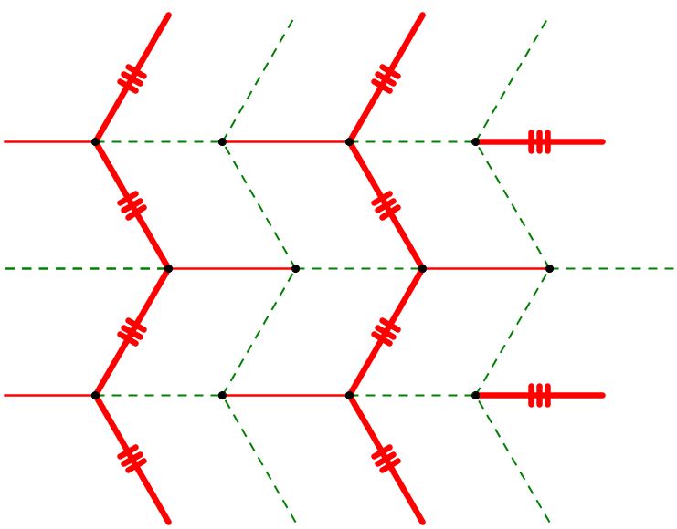
We assume at first that the Miura-ori has an even number of columns—which is to say, an odd number of zig-zags. We tile it with horizontal dominoes (see the left four columns of Figure 4a). Each domino crosses exactly one crease of the Miura-ori. With this particular tiling and MV assignment, we see that every mountain zig-zag crease path (and no other crease) is completely covered by dominoes; let consist of these creases. By Corollary 1, is a forcing set for .
Now suppose that the Miura-ori has an odd number of columns, but an even number of rows. We tile the rightmost column (“column ”) with vertical dominoes, and the rest of the grid as before. We have again covered every mountain zig-zag crease path, and also the horizontal mountain creases (middle toes) in column . With this choice of , we see that is determined for all creases except, perhaps, the valley creases in column and its bounding zig-zag. Since is forced in column , the creases that appear there as valleys are indeed forced to be valleys. These give us a valley leg and mountain toes at alternate nodes adjacent to column —which, by Corollary 1, forces on the rightmost valley zig-zag and therefore throughout the map.
When the Miura-ori has an odd number of rows and columns, we omit the bottom-right cell from the tiling, but otherwise proceed as above—tiling column with vertical dominoes, and the rest with horizontal dominoes. The collection of mountain creases corresponding to this domino tiling is sufficient to force everywhere except for the two creases bounding the bottom-right cell. Around their common node, we know that one toe is a mountain crease and another a valley, but now flat-foldability requires only that the remaining toe and leg agree with each other: they could be both mountains or both valleys. Thus, we add one of these creases to in order to force the standard MV assignment across the grid.
Suppose that is a forcing set corresponding to a domino tiling in which some square is covered by a pair of parallel dominoes. Let be the crease set corresponding to the domino tiling that results when these two parallel dominoes are flipped: turn a horizontal pair vertical, or vice-versa. Corollary 1 implies that is also a forcing set. Furthermore, all domino tilings of the Miura grid are flip-connected [17], so any domino tiling of the grid (in which is even) corresponds to a forcing set of size . Thus we have the following result.
Theorem 3.
When is even, an Miura-ori crease pattern with the standard MV assignment has a minimum forcing set of creases.
Proof.
The domino tiling procedure presented above produces a forcing set of creases. To show that this is of minimum size, it is easily verified that negating the standard MV assignment along the boundary of a single cell (turning two mountains into valleys and two valleys into mountains, for an interior cell) produces a new MV assignment that satisfies conditions for local flat-foldability. Therefore, a set must contain at least one crease of each cell in order to force . As a crease may serve this purpose in up to two cells, a forcing set must contain at least creases. This implies that all of the forcing sets based on domino tilings are minimum for the standard MV-assignment. ∎
For non-standard MV assignments, domino tilings are not guaranteed to produce forcing sets. For example, consider a single bird’s foot with the flat-foldable assignment , and . A domino tiling covers creases , but fixing the MV assignments of these two creases does not force the assignments of the remaining two creases; the other two creases could both be +1 or they could both be -1 for flat-foldability. Therefore, in the remainder of the paper we consider the more challenging problem of finding forcing sets for an arbitrary flat-foldable MV-assignment.
5 Tight Bounds for Non-Standard Miura-ori
Throughout this section, we view an 3-colored grid graph as an grid of squares with colored vertices placed at their centers. We maintain the term edge to refer to an edge connecting two adjacent square centers (see the dashed edges in Figure 5a), but distinguish it from an arc, which refers to an edge of the square grid (see the solid edges in Figure 5a). Note that each edge crosses exactly one arc. We imagine each square having the same color as its center. Let be a 3-coloring of a given grid graph . For simplicity, we define for a square to be the same as , where is the center of .
A uniform curve of is a boundary-to-boundary path or cycle of interior arcs with the property that the color difference (mod 3) is the same across every arc of . In other words, for any two edges and crossed by , with and on the same side of , the equality holds. Figure 5b shows several uniform curves for the grid graph from Figure 5a. The term “uniform” is used to remind the reader that the color difference is uniform across each arc of . As we shall later see, there is a one-to-one correspondence between the set of forcing edges and the set of uniform curves in . The following property follows immediately from the definition of a uniform curve.
Property 1.
Let and be the two colors across an arc of a uniform curve , and let . Now adding either to all colors on the same side of as , or to all colors on the same side of as , yields another valid coloring.
Corollary 2.
Any forcing set for must include an edge across every uniform curve in .
If no edge in a forcing set cuts across a uniform curve , then we can modify the coloring by adding or to all colors on one side of and get a different valid coloring (by Property 1), contradicting the fact that is forcing.
5.1 Minimum Forcing Set Algorithm
Before describing an algorithm for finding a minimum forcing set of a 3-colored grid graph , we provide some intuition behind our approach to force a particular coloring on .
Let and be two arbitrary -colorings of (ignoring for now forced edges). We encapsulate the difference between and in a graph with the same structure as , which we refer to as the difference graph. This graph is obtained by partitioning into maximal polyominoes of three types: -polyominoes include squares such that ; -polyominoes include squares such that ; and -polyominoes include squares such that . A -square, with , is a square in the difference graph that belongs to a -polyomino. Figure 6c shows the difference graph corresponding to the two colorings from Figures 6a and 6b. We view the square types , and as colors and seek to partition the polyomino boundaries into a collection of uniform curves, meaning that the color difference across each arc of such a curve is uniform. These uniform curves will guide us into selecting a set of edges that forces on .
In order to determine a partition of polyomino boundaries into uniform curves, we need to examine the way these boundaries intersect. Because a polyomino is composed of adjacent squares, the boundaries of two different polyominoes may not cross; they may, however, share square corners. Two adjacent polyominoes clearly share square corners, but it is also possible for three or four polyominoes to share a square corner (see square corners labeled and in Figure 6c, incident on three and four polyominoes, respectively). Call a square corner where three or four polyominoes meet a hub; these are marked by thick red dots in Figure 6c.
Observation 1.
At any hub , two diagonally opposite squares incident on must be of the same type and the other two squares incident on may be of either the same or different types.
To verify this observation, assume to the contrary that both pairs of diagonally opposite squares are of different types. Then two squares of the same type incident on are adjacent. For simplicity, assume that these are -squares, so they have matching colors in and (the argument is symmetric for a different choice of square type). Then the other two squares incident on are also adjacent and therefore must be of different types (otherwise we would have only two polyominoes incident on ). Let and be the colors in and corresponding to the -square incident on . Refer to Figure 7a. Then the colors in and corresponding to the -square must be and respectively, because any other pair of colors would result in adjacent identical colors, contradicting the fact that and are both valid colorings. This leaves as the only color available for the two adjacent -squares incident on , again in contradiction with the fact that and are valid colorings.
Observation 1is crucial in deciding how a uniform curve turns at a hub. It tells us that, if squares of three different types meet at a hub , then two diagonally opposite squares are of different types, and the other two diagonally opposite squares are of the same type. In this case we smooth to two right angles corresponding to the squares of different types incident on (see Figure 7b). This leaves the two squares of the same type to the same side of each right angle, as required along each segment of a uniform curve. If the two squares of the same type incident to are in different polyominoes before smoothing , then we view the two polyominoes as merging into a single one after smoothing . If squares of only two types meet at a hub , then any pair of diagonally opposite right angles can be used to smooth out , because the other two squares are guaranteed to be of the same type. Figure 7c shows the result of smoothing all the hubs in the difference graph from Figure 6c.
Once all hubs have been eliminated by this smoothing process, the union of all polyomino boundaries contains only pairwise disjoint components. These components are precisely the uniform curves in the graph formed from the difference between and . (See Figure 7d.)
Observation 2.
For each uniform curve in , the difference between two colors across an arc of is different in and .
To see this, pick an arbitrary uniform curve and let and be the two polyominoes adjacent to either side of in the graph formed by the difference between and . Pick an arbitrary arc of , and let and be the two adjacent vertices on either side of . We now consider all possible combinations of polyomino types. If is a -polyomino, then is either a or a -polyomino. In the first case we have , and because , we get . In the latter case, the argument is symmetric with replaced by . Finally, if is a -polyomino and is a -polyomino, we have , , which together yield . This settles Observation 2.
Lemma 1.
Let be a set that includes, for every uniform curve in , an edge across with its end vertices colored according to . Then does not agree with the coloring imposed by .
Proof.
Let be an arbitrary uniform curve in the difference graph . By the lemma statement, includes an edge across such that the difference between the colors of and equals . By Observation 2, , therefore does not respect . ∎
The Algorithm.
Next we describe an time algorithm that determines a minimum forcing set of a given -colored grid graph . Let denote the coloring function for .
The algorithm consists of two main steps. In a first step we derive from a planar directed graph that encapsulates all uniform curves of . In a second step we select from a minimum set of edges whose removal leaves acyclic, and show that this is a minimum forcing set for . Algorithm 1 outlines the key steps of this algorithm.
1. Compute the directed graph :
We now turn to describing the first step in detail. The graph has one node for each interior square corner of , and one node for the whole outer boundary of . Refer to Figure 8. The edges of are the interior arcs, with those incident to the outer boundary extended to meet the representative node.
For every pair of squares and adjacent along an arc , we orient clockwise around if , and counterclockwise otherwise. (Note that swapping the roles of and does not change this rule for directing arcs.) The construction of is linear in the size of , which is .
Observation 3.
Every directed cycle of is a uniform curve.
This observation follows immediately from the fact that all arcs have the same orientation along a directed cycle in . This means that the difference (mod 3) between the two colors across every arc of must be the same (either across all arcs, or across all arcs), otherwise two arcs along would have opposite orientations.
Lemma 2.
For any coloring , the set of directed cycles in includes all uniform curves in the difference graph .
Proof.
Pick an arbitrary uniform curve in . By definition, the color difference is the same across every arc of . This implies that all arcs of are oriented the same way in and therefore is a directed cycle in . ∎
Figure 9a outlines the uniform curves in the difference graph from Figure 7c. Figure 9b outlines four other uniform curves that potentially correspond to different valid colorings of .
Theorem 4.
Let be a set of edges. Coloring is forced by if and only if includes an edge across every directed cycle of .
Proof.
To prove this theorem in the ‘if’ direction, assume that the coloring is forced by , but does not include an edge in every directed cycle of . Let be such a directed cycle. By Observation 3, is a uniform curve. By Corollary 2, every forcing set ( in particular) must include an edge across , a contradiction. To prove the theorem in the ‘only if’ direction, assume that includes an edge across every directed cycle of , but does not force . This implies that there exists another valid coloring that respects . By Lemma 2, each uniform curve in the difference graph is a directed cycle in . By the theorem statement includes an edge across each such directed cycle. This along with Lemma 1 implies that does not respect , a contradiction. ∎
Theorem 4 suggests that finding a minimum forcing set for can be reduced to finding a minimum feedback arc set in (that is, a minimum set of arcs whose removal leaves acyclic). This problem is known to be polynomial for the class of reducible flow graphs, which include planar digraphs [11, 16]. More precisely, a minimum feedback arc set in the planar digraph can be determined in time quadratic in the number of arcs in [16], which is . We use the solution to the minimum feedback arc set problem on to extract a minimum forcing set for : corresponding to each arc in the minimum feedback arc set for , we include in the edge crossing . By Theorem 4, is a forcing set for . The running time of the algorithm that determines is .
5.2 Lower Bounds for Non-Standard Miura-ori
In this section we show the existence of Miura-ori folding patterns whose forcing sets are of size exactly , the smallest possible for any Miura-ori pattern.
Theorem 5 (Lower Bound).
There exist grid graphs whose forcing sets require exactly edges. Here , refer to the number of vertices in a column or row, respectively, of the grid graph.
Proof.
Consider a grid graph with diagonal stripes of one of the three colors in cyclic order, as depicted in Figure 10a. Each boundary-to-boundary path running alongside a diagonal stripe of squares separates some color on one side from an adjacent color on its other side.
(See path marked in Figure 10b, which separates colors and .) Such a path is a uniform curve, and by Corollary 2 it must be crossed by an edge in the forcing set. The number of such uniform curves is exactly , because each crosses exactly two of the boundary edges. Because these diagonal paths (and therefore the sets of edges they cross) are pairwise disjoint, the forcing set must include at least as many edges as the number of uniform curves, which is . ∎
This bound is tight, as for any Miura-ori folding pattern, every boundary arc must be part of one of the uniform curves, each uniform curve can only include two such arcs, and each curve must be crossed by a forcing set. Therefore, there can be no pattern requiring fewer than edges in its smallest forcing set.
5.3 Upper Bounds for Non-Standard Miura-ori
In this section we give a simple time algorithm that establishes an upper bound of on the size of a forcing set for any flat-foldable MV-assignment, making the standard Miura-ori in a sense the worse case. In this section we again make use of the grid graph representation of the Miura-ori discussed in Section 3.
Theorem 6.
Given any locally flat-foldable MV assignment of a Miura-ori crease pattern, there is an algorithm that finds a forcing set of size in time .
Proof.
Let be the -colored grid graph corresponding to the Miura-ori MV assignment with the color of the upper-left vertex fixed to 0. We create a forcing set for by assigning an orientation to the edges in two rows at a time from top to bottom, and within each pair of rows we work left to right. When done, the set will be a set of directed edges. Each directed edge with source and destination has weight of such that , where is the color of vertex .
We will assume that (the number of rows) is even; the algorithm is the same when is odd, with just a minor modification (not discussed here) to handle the last row. Starting with the top two rows, we begin by adding to the vertical edge directed from the upper-left vertex to the one below. Because the color of the upper-left vertex is fixed to 0, this forces the color of the vertex below it. We then look at each successive block formed by two already-forced vertices , and the two new vertices to the right of them. If it is a -colored block, then adding to the directed edge with its associated weight is enough to force the colors of the new vertices. (See Figure 11a.) It is easy to verify that the only coloring for the new vertices that is consistent with the added forcing edge and the already forced colors of vertices is one in which and . If the block is -colored, then one of the two new vertices has neighbors of both colors within the block. (See vertex in Figure 11b.) In this case, adding to the horizontal edge connecting an already forced vertex to the new vertex that does not have neighbors of both colors is enough to force the colors of the new vertices.
After forcing all colors on a pair of rows in this manner, we transition to the next row pair below it by looking at the block formed by the first two vertices on the bottom row of the previous row pair and the first two vertices on the top row of the new row pair. Because the top two vertices in the block are already forced, we can apply the same rules from above to add one edge to that forces the two lower vertices in the block. (Note that the correctness of the block rules does not depend on which pair of adjacent vertices in the block are already forced.) We do this again with the first block of the new row pair, and from there continue left to right across the new row pair as before. This repeats until all row pairs have been colored, so the algorithm completes in time linear in the size of , which is .
When processing each block, we gain two new colored grid vertices for only one forced edge. Therefore the total number of forced edges is . (When and are both odd, we need the ceiling of this term because one edge is used to force the bottom right vertex.) With the established correspondence between grid graph colorings and Miura-ori crease pattern MV assignments, the forcing set of immediately gives a forcing set for the Miura-ori MV assignment where each forcing edge in is replaced by its dual crease. ∎
6 Forcing Set Characterization
In this section we describe algorithms for testing whether a given set is forcing for a given Miura-ori crease pattern and whether a given partial mountain-valley assignment can be completed to a locally flat-foldable Miura-ori. Combining these two results together will give us an efficient algorithm for the problem of, given a forcing set, determining the folding pattern that it forces.
6.1 From Grid Colorings to Eulerian Digraphs
The following lemma characterizes the locally flat foldable MV assignments (or equivalently 3-vertex-colorings of a grid) in terms of the properties of the digraph used in our algorithm for finding a minimum forcing set. The lemma will be used shortly in testing for forced local flat foldability (subsection 6.3).
Lemma 3.
Let be a grid graph. Then the construction of an Eulerian digraph from a 3-coloring of , in Step 1 of Algorithm 1, is a bijection between 3-colorings of (with a fixed choice of color for one vertex) and Eulerian orientations of the graph formed by adding one outer vertex to .
Proof.
Consider a block of squares and let be the color of the top left square in this block. Assume first that has a valid -coloring. The two squares adjacent to in this block can be of either the same or different colors. If they are of different colors, then the square diagonally opposite to must have color and the arc orientation is as shown in Figure 12a. If the two squares adjacent to have the same color (as in Figures 12b–12e), then there are two choices for the color of the square diagonally opposite to . All possible cases are depicted in Figure 12, and each of these cases yields the indegree and outdegree equal to 2 at the center node. This shows that is Eulerian.
In the other direction, if is Eulerian, then we can process block of squares, starting with the top left block, and assign colors to the block squares according to the patterns showed in Figure 12. We then look at each successive block formed by the right column of the previous block and the one to its right, so that each successive block includes two colored squares to guide the coloring of the other two squares. After coloring all squares in the first row pair, we transition to the next row pair formed by the bottom row of the previous pair and the one immediately below it, and continue this process. The final result is a valid -coloring of . ∎
6.2 Testing Whether a Set is Forcing
Given a -colored grid graph and a set of edges in , we can easily determine in time whether is a forcing set or not. To do so, we first derive from a directed graph as described in Step 1 of the minimum forcing set algorithm (see Algorithm 1). As mentioned earlier, this step takes time . Corresponding to each edge , we delete from the dual arc crossing . Let be the graph obtained from after removing all such arcs. Theorem 4 implies that is a forcing set if and only if is acyclic. Thus testing the forcing property for reduces to testing the acyclic property for , which can be accomplished by means of a simple depth-first traversal of in time .
6.3 Testing for Local Flat Foldability
Given an assignment of mountain/valley to a subset of the creases in a Miura-ori pattern, our goal in this section is to test whether there exists a locally flat-foldable fold on all pattern creases that is consistent with the input . We show that this task can be accomplished in time.
Let be the graph representation of the Miura pattern, with vertices interior to the squares of a grid (as in Figure 5a). Precolor the top left vertex of and assign weights or to all edges of associated with creases in , consistent with the MV assignment of the corresponding creases. Each edge not associated with a crease in has a null weight. Based on the correspondence between local flat foldability of the Miura-ori crease pattern and -colorability of (established in Section 3), testing for local flat-foldability reduces to showing that has a valid -coloring that respects the non-null edge weights.
Let be the directed representation for derived as in Step 1 of the the minimum forcing set algorithm (see Algorithm 1). Note that arcs in corresponding to creases in will be oriented in , but the rest of them start as undirected arcs. See Figure 13a for an example. By Lemma 3, has a valid -coloring if and only if can be extended to a directed Eulerian graph in which every node (with the exception of the outer node) has in degree and out degree equal to . Thus our goal is to orient all undirected arcs of such that the resulted graph is directed Eulerian.
To determine an Eulerian orientation for , we set up a network flow on the undirected arcs of , where each arc has capacity in both directions. Corresponding to each arc directed from to in , we add one unit of demand at the tail and one unit of supply at the head . Thus the total supply equals the total demand. Figure 13b shows the flow network corresponding to the directed graph from Figure 13a; negative values at nodes indicate demand and positive values indicate supply. We need to determine a feasible flow from supply nodes to demand nodes that satisfies the demands at all nodes, subject to the unit capacity constraints. Because there are no sources or sinks involved here, determining a feasible flow in reduces to finding a circulation in , which can be accomplished in time using Miller’s algorithm (see section 4 in [13]). If there is no solution to the flow problem, then there is no locally flat-foldable fold on all pattern creases that is consistent with the input. Otherwise, the solution to the flow problem is an Eulerian orientation that includes all the input creases. Figure 14a shows an Eulerian orientation that satisfies the supply and demand requirements for the flow network depicted in Figure 13b.
The Eulerian orientation determined in the previous step includes all creases in the input set , but it may leave some arcs in undirected. Let be the subgraph of consisting of all undirected arcs (it may have several connected components). Each node in has even degree, therefore is an Eulerian undirected graph. By Veblen’s theorem [18], can be partitioned into simple disjoint cycles. This can be accomplished in time linear in the number of graph arcs, which is . Choose an arbitrary orientation for each cycle. (See Figure 14b for an example.) The result is the desired Eulerian orientation on the whole graph . (See Figure 15a, which combines the arc orientations from Figures 13a, 14a and 14b.)
From the Eulerian orientation of we determine a -coloring of the grid graph following the approach used in Step 1 of the minimum forcing set algorithm (Algorithm 1): if an arc shared by squares and is oriented clockwise around , then , otherwise . Figure 15a shows the correspondence between the -coloring and the Eulerian orientation of . Finally we use the established correspondence between a -coloring of the grid graph and a folding pattern to determine a mountain/valley assignment for the all creases, consistent with the input . Figure 15b shows the mountain/valley assignment corresponding to the -coloring from Figure 15a.
7 Tight Controlling Sets
This section introduces the notion of controlling forcing sets, and gives tight bounds on the size of controlling sets for the Miura-ori crease pattern. For a given crease pattern , a subset is controlling forcing, or simply controlling, if it is forcing for every mountain-valley assignment on .
As we show in this section, controlling sets for Miura-ori must be significantly larger than forcing sets for particular MV-assignments.
Theorem 7.
A subset of the Miura-ori creases is controlling if and only if it contains a spanning tree of the dual grid graph.
Proof.
In one direction, if contains the creases corresponding to the edges of a spanning tree in the dual grid graph, it is easy to show that is forcing by propagating colors along the tree from the fixed color in the top left corner.
In the other direction, if the grid graph edges corresponding to do not span the entire grid graph, then we show that there exist two valid checkerboard colorings that cannot be distinguished by and therefore is not a forcing set. Figure 16 shows an example where induces two or more connected components in the grid graph, one of which consists of the vertices in the shaded L-shaped region. For the first checkerboard pattern, we assign every other vertex of the grid graph the color 1. Then we pick an arbitrary component and assign its remaining vertices the color 2, while everywhere else we assign the remaining vertices the color 0, as illustrated in Figure 16a. For the second pattern, we change the 1-2 checkerboard pattern of the selected component to 2-0 (see Figure 16b). This preserves the validity of the coloring and cannot be distinguished by a supposed forcing set that includes no edges between the component’s vertices and the rest of the graph. ∎
8 Conclusions
Inspired by the need to reduce the cost of pre-programmed self-folding mechanisms, we study forcing sets for the classical Miura-ori folding pattern. We present efficient algorithms for determining a minimum forcing set of a Miura-ori map (Sections 4 and 5), and for extending a given MV assignment to a forcing set, if possible (Section 6). We also introduce the notion of controlling forcing sets, and give tight bounds on the size of controlling sets for the Miura-ori crease pattern (Section 7).
Our work opens several new questions, chief among which stands the question of global flat-foldability. It would be interesting to determine if the MV-assignments induced by some of the algorithms in this paper are globally flat-foldable or not. Extending the results beyond the confines of the Miura-ori crease pattern remains open.
References
- [1] B. An, N. M. Benbernou, E. D. Demaine, and D. Rus. Planning to fold multiple objects from a single self-folding sheet. Robotica 29:87–102, 2011, doi:10.1017/S0263574710000731.
- [2] E. Arkin, M. A. Bender, E. D. Demaine, M. L. Demaine, J. S. B. Mitchell, S. Sethia, and S. Skiena. When can you fold a map? Comput. Geom. Theory Appl. 29(1):166–195, 2004, doi:10.1016/j.comgeo.2004.03.012.
- [3] M. Bern and B. Hayes. The complexity of flat origami. Proc. 7th ACM-SIAM Symposium on Discrete Algorithms (SODA ’96), pp. 175–183, 1996.
- [4] E. D. Demaine and J. O’Rourke. Geometric Folding Algorithms: Linkages, Origami, Polyhedra. Cambridge University Press, 2007.
- [5] J. Ginepro and T. Hull. Counting Miura-ori foldings. Preprint, 2014.
- [6] E. Hawkes, B. An, N. M. Benbernou, H. Tanaka, S. Kim, E. D. Demaine, D. Rus, and R. J. Wood. Programmable matter by folding. Proceedings of the National Academy of Sciences 107:12441–12445, 2010, doi:10.1073/pnas.0914069107.
- [7] T. Hull. Counting mountain-valley assignments for flat folds. Ars Combin. 67:175–188, 2003.
- [8] T. Hull. Project Origami: Activities for Exploring Mathematics. A K Peters, Wellesley, MA, 2006.
- [9] L. Ionov. 3D micro fabrication using stimuli-responsive self-folding polymer films. Polymer Reviews 53(1):92–107, 2013, doi:10.1080/15583724.2012.751923.
- [10] T. G. Leong, P. A. Lester, T. L. Koh, E. K. Call, and D. H. Gracias. Surface tension-driven self-folding polyhedra. Langmuir 23(17):8747–8751, 2007, doi:10.1021/la700913m.
- [11] C. L. Lucchesi. A minimax equality for directed graphs. Ph.D. thesis, University of Waterloo, Ontario, Canada, 1976.
- [12] L. Mahadevan and S. Rica. Self-organized origami. Science 307(5716):1740, 2005, doi:10.1126/science.1105169.
- [13] G. L. Miller. Flow in planar graphs with multiple sources and sinks. SIAM J. Comput. 24(5):1002–1017, 1995, doi:10.1137/S0097539789162997.
- [14] T. Morgan. Map Folding. Master’s thesis, Mass. Inst. Tech., 2012.
- [15] R. I. Nishat and S. Whitesides. Map folding. Canadian Conf. on Comp. Geom., pp. 49–54, 2013, http://www.cccg.ca/proceedings/2013/papers/paper_49.pdf.
- [16] V. Ramachandran. Finding a minimum feedback arc set in reducible flow graphs. J. of Algorithms 9(3):299–313, 1988, doi:10.1016/0196-6774(88)90022-3.
- [17] N. C. Saldanha, C. Tomei, M. A. Casarin, Jr., and D. Romualdo. Spaces of domino tilings. Discrete Comput. Geom. 14(1):207–233, 1995, doi:10.1007/BF02570703.
- [18] O. Veblen. An application of modular equations in analysis situs. Ann. Math. 14(1):86–94, 1912, doi:10.2307/1967604.