Inherent Structures in -component Spin Glasses
Abstract
We observe numerically the properties of the infinite-temperature inherent structures of -component vector spin glasses in three dimensions. An increase of implies a decrease of the amount of minima of the free energy, down to the trivial presence of a unique minimum. For little correlations are small and the dynamics are quickly arrested, while for larger low-temperature correlations crop up and the convergence is slower, to a limit that appears to be related with the system size.
I Introduction
Although it is established that typical spin glasses [1] order at a critical temperature for [2, 3, 4], the nature of the low-temperature phase of spin glasses under the upper critical dimension is still a matter of debate [5, 6, 7]. There are two main theories describing the spin glass phase.
(1) The droplet theory portrays spin glasses as disguised ferromagnets, with only two low-temperature states, and no spin glass phase once an external magnetic field is applied [8, 9, 10]. Ferromagnets in disguise can be obtained, for example, by performing a random gauge transformation on an ordered system [11], as it is done in the Mattis model [12].
(2) On the other side the replica symmetry breaking (RSB) theory characterizes the spin glass phase with a rugged free-energy landscape with an exponentially large number of states with an ultrametric structure [13, 14, 15]. Once the temperature is lowered under the critical point, the phase space is split up in many regions separated by barriers that diverge with the system size, so ergodicity is broken. When a field is applied, at high dimensions a critical line (the dAT line [16]) separates the spin glass from the paramagnetic phase. In low enough dimensions both the transition at and disappear.
At the present moment the lower critical dimension at seems to be around . Its value in a field, instead, is still matter of debate: The situation could be similar to that of a ferromagnet where the lower critical dimension in absence of a field (i.e. 1) is different from the lower critical dimension in the presence of a random field (i.e. 2).
Since increasing the number of spin components reduces the number of metastable states, recent works focused on the properties of these models in the limit, and their energy landscape [17]. Interesting features have been pointed out in large- mean field models, such as a Bose-Einstein condensation in which the spins condense from an -dimensional to an -dimensional subspace, with [18].
It has been argued in Ref. 18 that the limit could be a good starting point for the study of the low- spin glasses [19], via expansions that have been used, for example, to try to question the presence of a dAT line [20]. However the Hamiltonian of the model has a unique local minimum, that can be found easily by steepest descendent (the determination of the ground state is not an NP complete problem).
Explicit computations also indicate that the model is substantially different from any finite- model (for example there is only quasi long-range order under , the upper critical dimension has been shown to be , and the lower critical dimension is suspected to be too [21, 22, 23]), and that it is more interesting to study these models for large but finite , thus reversing the order of the limits and ( is the total number of spins) [23].
To better understand the large (but finite) limit we undertake a numerical study in a three-dimensional cubic lattice. Our aim is to arrive at a quantitative comprehension of the energy landscape of systems with varying , expecting, for example, to observe growing correlations as increases [17].
We focus on infinite-temperature inherent structures, i.e. the local energy minima that one reaches by relaxing the system from an infinite-temperature state, that is equivalent to a random configuration. Examining a system from the point of view of the inherent structures is a very common practice in the study of structural glasses [24]. Only recently the study of quenches 11 1 By quench we mean the minimization of the energy throughout the best possible satisfaction of the local constraints, i.e. a quench is a dynamical procedure. In Sec. II we explain how the quenches were performed. Be careful not to confuse it with other uses of the same term. For example, those quenches have little to do with the quenched approximation used in QCD, or the quenched disorder, that is a property of the system. from a high to a lower temperature has stimulated interest also in spin systems, both in presence and absence of quenched disorder 22 2 Let us stress once again the meaning of the term quench, since the terminology might generate some confusion. We refer to quenched disorder when the system is described by some random variables that do not change in time. This concept is independent from the quenches we impose to our system, i.e. relaxing the system to the closest local minimum of the energy. [25, 26, 27].
We analyze the properties of the inherent structures, and we inspect the dynamics of how the system converges to those configurations.
When one performs a quench from to , the system is expected to show two types of dynamics, an initial regime where thermal fluctuations are irrelevant, and a later one where they dominate the evolution (see for example the quenches performed in Ref. 26). We choose , so we can to show that the origin of the second dynamical regime is actually due to thermal effects. We study the quenches as a function of . While on one side in the Ising limit the dynamics is trivial, and correlations never become larger than a single lattice spacing, on the other side an increasing yields a slower convergence, with the arising of low-temperature correlations that we can interpret as interactions between blocks of spins.
The paper is structured as follows. In Sec. II we define our model and describe how simulations were done. In Sec. III we define the observables we measured, and in Sec. IV we show our numerical results. First we analyze the properties of the inherent structures as a function of , and then we show the time evolution of the observables during the quenches. Conclusions are given in Sec. V. In the Appendix we show a simple example of how the selfoverlap can depend on .
II Model and Simulations
II.1 Model
The model is defined on a cubic lattice of side with periodic boundary conditions. Each of the vertices of the lattice hosts an -dimensional spin , with the constraint . Neighboring spins and are linked through a coupling constant . The Hamiltonian is
| (1) |
where the brackets indicate that the sum goes only over the nearest neighbors. The spins are our dynamic variables, while the couplings are Gaussian-distributed, with and . We define different realizations of the couplings in a lattice with the term samples. Independent configurations of the spins that have the same couplings are called replicas of the same sample. This Hamiltonian is invariant under the simultaneous rotation or reflection of all the spins [that belongs to the symmetry group], so the energy minimas may be found modulo a global rotation.
II.2 Simulations
We are interested in the inherent structures from infinite temperature, hence we need to pick random starting configurations, and directly minimize the energy. 33 3 The couplings and the initial configurations were chosen at random with a combination of congruential and Parisi-Rapuano random number generator.[38, 39]
The algorithm we choose is a direct quench, that consists in aligning each spin to its local field . 44 4 The local field is defined as . This choice was done because it allows us to compare inherent structures from systems with a different in a general way, 55 5 For example, the Successive Over Relaxation used in Ref. 27 yields inherent structures with different properties, depending on the value of a parameter , and the same is not equivalent for two different values of . because it is the most simple and widely used in literature, and because it leads to inherent structures that are conceptually mostly similar to those conceived in the field of supercooled liquids.
For each sample we simulated two replicas, in order to be able to compute overlaps. We fixed the number of full sweeps of a lattice to , as it had already been done in Ref. 26 with quenches to finite temperature. This amount of steps was enough to guarantee the convergence to an inherent structure in all our simulations. To ensure the convergence we required the last (logarithmically spaced) measurements to be equal within the error for each of the measured observables.
In Tab. 1 we give the parameters of our simulations.
| 8 | 1 | 10000 | 22 | |
| 8 | 2 | 10000 | 22 | |
| 8 | 3 | 10000 | 22 | |
| 8 | 4 | 5000 | 22 | |
| 8 | 6 | 10000 | 22 | |
| 8 | 8 | 10000 | 22 | |
| 16 | 1 | 1000 | 22 | |
| 16 | 2 | 1000 | 22 | |
| 16 | 3 | 1000 | 22 | |
| 16 | 4 | 1000 | 22 | |
| 16 | 8 | 1000 | 22 | |
| 16 | 12 | 1000 | 22 | |
| 16 | 16 | 1000 | 22 | |
| 64 | 3 | 160 | 22 |
III Observables
We will use two replicas in order to create gauge-invariant observables.[1] To identify different replicas we use the superscripts (a) and (b). The site overlap is defined as
| (2) | |||||
The order parameter is the overlap tensor:[28]
| (3) |
This quantity is not rotationally invariant, so we will use the square overlap [29, 30]
| (4) | |||||
All the eigenvalues of are rotationally invariant.
Throughout the article, when we will be talking of overlap, we will be referring to the defined in Eq. (4). The selfoverlap is defined analogously, by taking in the previous definitions. Notice that the selfoverlap is not identically equal to 1. It is easy to see, for example, that at infinite temperature, in the thermodynamic limit it is equal to (see the Appendix).
We will be measuring both point and plane correlation functions. The point correlation function is
| (5) |
where (or ), 2 (or ), 3 (or ) is a coordinate axis, and is the unitary vector in that direction. We also use plane correlation functions because they decay slower and have a better signal-to-noise ratio. If we denominate the plane-overlap tensor as the mean overlap tensor over a plane
| (6) |
we can define the plane correlation function as
| (7) |
Both definitions of are invariant. From the correlation functions we measure the second-moment correlation lengths
| (8) | ||||
| (9) |
The difference in the definitions is due to the presence of a Jacobian term when we want to integrate the point correlation function over the space. These two lengths would be proportional by a factor if they had the same purely exponential correlation function. Note that and are proper estimators of a correlation length only when the correlation functions and are connected (i.e. they go to zero for large ). Otherwise, in principle they could be used to individuate if a quench penetrated in the spin glass phase. In fact, depending on a quench will drive us in a ferromagnetic or in a spin glass phase. Our correlation functions are connected in the spin glass phase, but they are not in a ferromagnetic state. Consequently, a cumulant such as will diverge as (see Ref. 35 for a definition of and an explanation of this behavior) when is too large for a spin glass phase, it will converge as if the quench penetrates in the spin glass phase, and it will be of order 1 right at the critical , , that is probably not integer, so not exactly locatable.
When the correlation function decays very quickly and the noise becomes larger than the signal, one could measure negative values of , that would be amplified by the factors and in the integrals. This would imply very large errors in , or even the square root of a negative number. To overcome this problem, we truncated the correlation functions when they became less than three times the error.[37] This procedure introduces a small bias, but reduces drastically the statistical error. Furthermore, the plane correlation function required the truncation much more rarely, therefore we compared the behaviors as a consistency check.
We also measured the link overlaps
| (10) | ||||
| (11) |
that were shown to be equivalent to the overlaps in the description of the low temperature phase.[36, 34] The link correlation functions are
| (12) | ||||
| (13) | ||||
| (14) |
The definitions of the link correlation lengths and are analogous to Eqs. (8) and (9).
Finally, since we also report measurements of the energy , let us stress that we used the Hamiltonian defined in Eq. 1, with a normalization factor, in order to bound it to one.
Throughout the article, each time one of the defined quantities is referred to the inherent structures (i.e. the final configurations of our quenches), we will stress it by putting the subscript IS.
IV Results
IV.1 Dependence on the number of components
We want to analyze how the model’s behavior changes with . Intuitively, the more components a spin has, the easier it is to avoid frustration 66 6 Frustration is the impossibility of satisfying all local constraints at the same time. A way to define it is through the Wilson loop [31]. For each closed circuit in the lattice, we can take the ordered product of all the links that form it. If this product is negative it is not possible to find a configuration that minimizes simultaneously the local energy along each of the links, and the loop is said to be frustrated [32]. When we talk about the system being more or less frustrated we refer to the presence of a larger or smaller number of frustrated loops. [17], and the simpler is the energy landscape.According to this scenario, when increases, the number of available inherent structures decreases down to the limit in which the energy landscape is trivial, and there is only one minimum. This should be reflected in the quantity , that should be small when there are many minima of the energy, and go to 1 when there is only one inherent structure, since all the quenches end in the same configuration. As shown in Fig. 1 (top), our expectation is confirmed. With Ising spins () the energy landscape is so rich that inherent structures have practically nothing in common. When we increase the overlaps start to grow until the limit . By comparing the data for different , we can dismiss a difference in the behavior between discrete () and continuous () spins, since for behaves the same as for . In Sec. IV.3 we will discuss aspects in which we do encounter differences.
Since the number of available inherent structures depends on both and , we can give an operative definition of a ratio under which the number of inherent structures is exponential (so ), and of a ratio over which there is only one minimum. This way, we can characterize finite-size effects effectively: An extremely small system is trivial and has only one stable state. Increasing the size we encounter a less trivial behavior, but to find a visible signature of a spin glass phase one has to have . From Fig. 1 one can see that for , , and for , . Then, for example, we see that to observe a complex behavior for spin glasses, one should use .
Moreover, this interpretation gives a straightforward explanation of the finite-size effects one encounters in the energy of an inherent structure (Table 2). For example, if we compare at , we notice two incompatible energies. In fact, there is an intrinsic difference between the two sizes, since represents single-basin systems, while has a variety of inherent structures. On the other side, finite-size effects on lower are smaller, because we are comparing similar types of behavior.
Notice that, although the ratio grows monotonously, this is not true for the pure overlap (Fig. 1, bottom), that has a peak at an intermediate . Moreover, the position of the peak doubles when we double the lattice linear size, justifying the operational definitions and .

The same peak at intermediate is also visible in the energy and in the correlation length (Fig. 2), indicating that there is an intrinsic difference in the nature of the reached inherent structures. In Table 2 we give the values of the aforementioned observables at the inherent structure.
| 8 | 1 | -0.4709(1) | 0.0095(1) | 1 | 0.68(2) | 1.71(1) |
|---|---|---|---|---|---|---|
| 8 | 2 | -0.5953(1) | 0.0497(3) | 0.50297(2) | 1.49(1) | 2.802(4) |
| 8 | 3 | -0.6151(1) | 0.1784(6) | 0.33994(4) | 2.188(2) | 3.2358(7) |
| 8 | 4 | -0.6176(2) | 0.2213(5) | 0.26229(9) | 2.2919(9) | 3.2760(5) |
| 8 | 6 | -0.61801(11) | 0.1989(1) | 0.1997(1) | 2.2567(3) | 3.2514(2) |
| 8 | 8 | -0.61797(12) | 0.1905(1) | 0.1905(1) | 2.2364(3) | 3.2428(2) |
| 16 | 1 | -0.4721(1) | 0.00123(6) | 1 | 0.63(2) | 1.69(1) |
| 16 | 2 | -0.5965(1) | 0.0067(2) | 0.500379(8) | 1.49(4) | 3.20(6) |
| 16 | 3 | -0.6165(1) | 0.0382(5) | 0.33416(1) | 3.37(3) | 5.43(1) |
| 16 | 4 | -0.6191(2) | 0.0833(6) | 0.25144(2) | 4.153(7) | 6.008(4) |
| 16 | 8 | -0.6200(1) | 0.1218(3) | 0.13126(5) | 4.519(2) | 6.187(1) |
| 16 | 12 | -0.6202(1) | 0.10031(9) | 0.10044(9) | 4.3814(8) | 6.087(1) |
| 16 | 16 | -0.6197(1) | 0.0959(1) | 0.0959(1) | 4.3412(8) | 6.066(1) |
| 64 | 3 | -0.61657(4) | 0.00064(2) | 0.3333466(4) | 3.53(7) | 6.74(6) |

We see in this behavior the competition between two effects. When is small, the quench has a vast choice of valleys where to fall. Since, reasonably the attracion basin of the lower-energy inherent structures is larger, the wide variety of inherent structures will increase the probability of falling in a minimum with low energy and larger correlations. When increases, the number of available valleys decreases, so it is more likely that two different replicas fall in the same one. Yet, the quality of the reached inherent structures decreases, since the quench does not have the possibility to choose the lowest-energy minimum.
IV.2 Overlap Probability Densities
From these observations it is reasonable to think that overlap and energy of the inherent structures are correlated. We looked for these correlations both on the overlap, on the selfoverlap, and in their ratio, but with a negative result. In Fig. 3 we show a scatter-plot of the ratio of the inherent structure’s overlaps that confirms our statements.
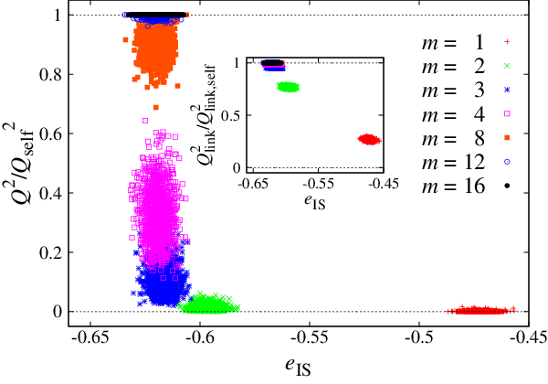
The cross sections of Fig. 3 give an idea of the energy and overlap probability distribution functions. We show explicitly the overlap probability distribution functions (normalized with the bin width) of the inherent structures in Fig. 4.

They are qualitatively different from their thermal counterparts (see, e.g., Ref. 35). The ratio is bounded between zero and one. The distributions are extremely wide, and the phenomenology is quite different near the two bounds. In fact, when is large enough, the limit changes completely the shape of the curves, introducing a second peak (that we could read as an echo of the Bose-Einstein condensation remarked in Ref. 18). Around the lower bound of the , instead, there is no double peak. We can try to give an interpretation to the presence of this second peak by looking at the overlap distribution functions for a given instance of the couplings. In Fig. 5 we show that this distribution has relevant sample-to-sample fluctuations. When we increase , the number of minima of the energy, , gradually becomes smaller. Yet, depending on the specific choice of the couplings, can vary sensibly. For example in Fig. 5, top-right, one can see that when and , can be both large (red curve) or of order one (blue curve). For , (Fig. 5, bottom-left), the situation is similar: for the blue curve , while for others .


As we similarly stated in Sec. IV.1, we notice that the lattice size plays a substantial role on the properties of the reached inherent structure, since when we pass from to histograms regarding the same cover very different ranges of . We can both see them traditionally as strong finite-size effects, or focus on as a relevant parameter (as it was suggested, for example, in Ref. 40), concentrating the interest on finite .
IV.2.1 Link Overlaps
Since in the past ten years an increasing attention has been devoted to the link overlap as an alternative order parameter for the study of the low temperature region of spin glasses,[33, 34, 35] in Fig. 6 we show also the link-overlap histograms ) at the inherent structures. The functions have much smaller finite-size effects than the , and are more Gaussian-like (although the Gaussian limit is impossible, since is bounded between 0 and 1). The inset shows that the second peak on high overlaps is present also with the link overlap.
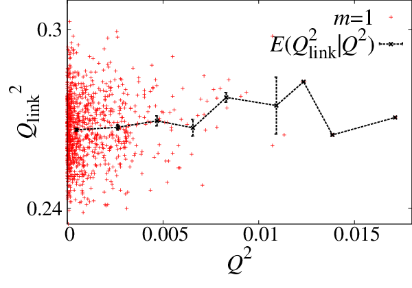
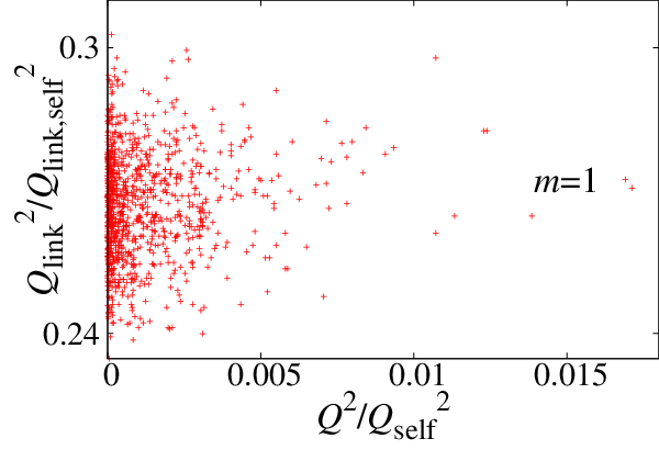
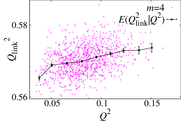
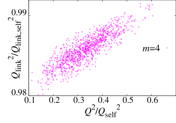
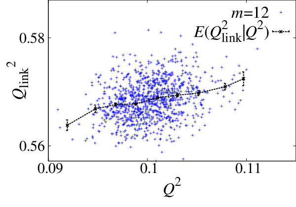
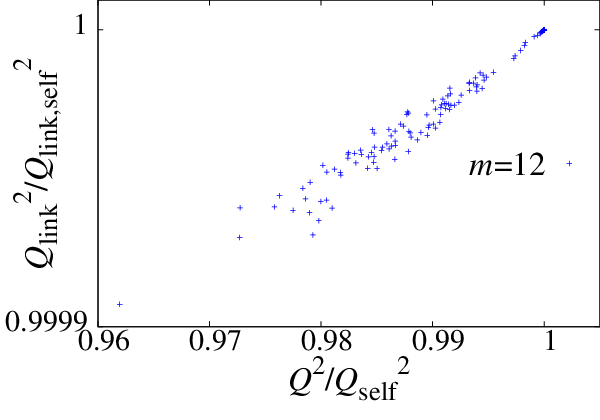
We checked also the correlation between spin and link overlaps. At finite temperature there are different predictions between RSB and droplet pictures. According to the RSB picture the conditional expectation value should to be a linear, strictly increasing function of , while this should not be true in the Droplet theory. When is small, this correlation is practically invisible, but it becomes extremely strong when we increase the number of components of the spins (Fig. 7). Notice how the correlation between spin and link overlap is formidably increased when we normalize the two with the selfoverlap. The curves in Fig. 7 represent . If we exclude the tails, that are dominated by rare non-Gaussian events, the trend is compatible with linearly increasing functions.

IV.3 Quench Dynamics
Let us get an insight on the dynamics of the quench. For short times, the energy converges towards a minimum with a roughly power law behavior (Fig. 8). At longer times there is a cutoff, that grows with the system’s size, revealing a change in the dynamics after which the system converges faster to a valley. We stress the great difference in the convergence rate between and . We can identify two different decrease rates, depending on whether the spins are discrete or continuous.

Fig. 9 shows the evolution of the overlap for , and gives a better understanding of why quantities such as are not monotonous with . We show both the evolution of (top), and of (bottom). The first one behaves as one would expects when the number of minima is decreasing to one. On the other side, we see from the lower plot how the quenches of reach the highest overlap. A possible interpretation is to ideally separate the quench in two regions. At the beginning there is a search of the valley with a power-law growth of , and later the convergence inside of the valley. Fig. 9 shows that the search of the valley stops earlier when , i.e. when their number is of order one.

We remark on a nonlinear trend on the evolution of the selfoverlap . For continuous spins () it has a different value at infinite and zero temperature (Fig. 10). This variation is strikingly visible when is large, but the same trends are found for , though the variations are so small that it is justified that they are usually not found. 77 7 To our knowledge, the only reference where a non-trivial behavior of the self-overlap was found is in Ref. 27. Yet, in this case it was in the study of inherent structures from finite temperature, and in the chiral sector (they worked with ). Moreover is highly nonlinear, and, except for the highest , it overshoots before having converged.

In Fig. 11 we show the evolution of the correlation lengths during the quenches for for all our values of . We see the same variety of behaviors shown by (Fig. 9), with that abruptly stop increasing, while when the increase is similar but lasts longer and the change of growth is smoother. 88 8 The point correlation length behaves analogously.
We can contrast our results with the ones obtained by Berthier and Young in Ref. 26 for Heisenberg spin glasses. In that case they measured the evolution of the coherence length in quenches down to positive temperature (). They remarked two different regimes of growth of the coherence length, and attributed them to the passage from critical to activated dynamics 99 9 Note that the definition of the coherence length in Ref. 26 is different from ours.. In that case the slope of the second phase kept being positive and did not appear to converge after lattice sweeps. We can make a direct comparison with our quenches to zero-temperature with (Fig. 9, inset). We obtain a flat second regime after sweeps, so we can indeed attribute the growth in the second regime to thermal effects. In the inset we compare the coherence length of different lattice sizes to remark that although , we are clearly far from the thermodynamic limit even for .

V Conclusions
We performed an extensive study of the energy landscape of three-dimensional vector spin glasses, focusing on their dependence on the number of components of the spins. We were concerned both with the zero- dynamics and with the properties of the inherent structures, remarking various types of finite-size effects.
Increasing the number of minima in the energy landscape decreases monotonously, down to the limit of a single state. The number of components after which the number of minima becomes subexponential grows with the lattice size. Reversing the relation, we can operatively define as the smallest lattice size needed in order to observe a complex behavior for a given .
For small correlations are small and dynamics are trivial, while when becomes larger correlations increase and the convergence to an inherent structure slows down (for a small enough ratio). We remark on the competition between the limit, with abundance of inherent structures, and the large- limit where at there is only a single state.
In finite systems neither the overlap, nor the correlation length, nor the energy of the inherent structures is a monotonous function of , as one would expect from a decreasing number of available disordered states. They have instead a peak at an intermediate . We attribute this to the fact that when there are several minima, those of more ordered states have a larger attraction basin, so having many inherent structures makes it easier to fall into a more ordered state. If one wanted to rule out the non-monotonous behavior it could be useful to redefine the correlations as a function of the normalized overlaps , as we have seen that the normalized overlaps do exhibit a monotonous trend.
Also, we presented probability distribution functions (pdf) of the spin and link order parameters and , noticing that the states with have a major attraction basin, and create a second peak in the curve. Finite-size effects in the inherent structures’ pdfs were very heavy, as remarked also by looking at other observables, but they were minimal if we considered the link overlap. Also, the dependency between and is consistent with RSB predictions.
Finally, we found a non-trivial behavior on the evolution of the self-overlap, that could be used as an indicator of the “quality” of a reached inherent structure.
Acknowledgements
We thank Víctor Martín-Mayor for useful conversations and a careful reading of the manuscript.
We were supported by the European Research Council under the European Union’s Seventh Framework Programme (FP7/2007-2013, ERC grant agreement no. 247328). We were partly supported by MINECO, Spain, through the research contract No. FIS2012-35719-C02. This work was partially supported by the GDRE 224 CNRS-INdAM GREFI-MEFI. M.B.-J. was supported by the FPU program (Ministerio de Educación, Spain).
Appendix A Self overlap at infinite temperature
We show here the simple case of dependence on of the selfoverlap at infinite temperature.
From Eq. 4, imposing that , we have that
| (15) | |||||
| (16) |
The typical value of the scalar product at infinite temperature is trivially , since it is equivalent to a random component of an -dimensional unitary sphere. Therefore the expectation value of the selfoverlap for a configuration at infinite temperature is
| (17) |
This relation, that takes in account finite-size effects and was verified for random configurations, can be compared with the selfoverlaps of the inherent structures in Table 2 (and with Fig. 10), that are consistently different, since this observable has a non-trivial dependency on the temperature.
References
- [1] M. Mézard, G. Parisi and M. A. Virasoro, “Spin Glass Theory and Beyond” (World Scientific, Singapore 1987).
- [2] .H. G. Ballesteros, A. Cruz, L. A. Fernandez, V. Martín-Mayor, J. Pech, J.J. Ruiz-Lorenzo, A. Tarancon, P. Tellez, C. L. Ullod, and C. Ungil, Phys. Rev. B 62, 14237 (2000).
- [3] H. Kawamura and M.S. Li, Phys. Rev. Lett., 87 18 (2001).
- [4] L.W. Lee and A.P. Young, Phys. Rev. Lett. 90, 227203 (2003).
- [5] M.A. Moore and A.J. Bray, Phys. Rev. B 83 224408 (2011).
- [6] G. Parisi and T. Temesvari Nucl. Phys. B 858 293 (2012).
- [7] J. Yeo and M.A. Moore, Phys. Rev. E 86 052501 (2012).
- [8] D.S. Fisher and D.A. Huse, Phys. Rev. Lett. 56 1601 (1986).
- [9] A.J. Bray and M.A. Moore, 1987, Scaling theory of the ordered phase of spin glasses Heidelberg Colloquium on Glassy Dynamics (Lecture Notes in Physics no 275) ed. J.L. van Hemmen and I. Morgenstern (Berlin: Springer).
- [10] D.S. Fisher and D.A. Huse, Phys. Rev. B 38 386 (1988).
- [11] H. Nishimori, Gauge Theory of Spin Glasses. In: Statistical Physics of Spin Glasses and Information Processing, Oxford University Press (2001).
- [12] D.C. Mattis, Phys. Lett. A, 56(5),421 (1976).
- [13] G. Parisi, Phys. Rev. Lett. 43 1754 (1979).
- [14] G. Parisi, J. Phys. A: Math. Gen. 13 1101 (1980).
- [15] G. Parisi Phys. Rev. Lett. 50 1946 (1983).
- [16] J.R.L. de Almeida and D.J. Thouless, J. Phys. A 11, 73 (1978).
- [17] M. B. Hastings, J. Stat. Phys. 99, 171 (2000).
- [18] T. Aspelmeier and M. A. Moore, Phys. Rev. Lett. 92, 077201 (2004).
- [19] For example, in F. Beyer, M. Weigel and M. A. Moore, Phys. Rev. B 86, 014431 (2012), the infinite- limit is used to derive exact relations in the one-dimensional spin glass with power law interactions.
- [20] M.A. Moore, Phys. Rev. E 86, 031114 (2012).
- [21] J.E. Green, A.J. Bray and M.A. Moore, J. Phys. A 15, 2307 (1982).
- [22] L. Viana, J. Phys. A 21, 803 (1988).
- [23] L.W. Lee, A. Dhar and A.P. Young, Phys. Rev. E 71 036146 (2005).
- [24] A. Cavagna, Phys. Rep., 476 4, 51 (2009).
- [25] E.g. see T. Blanchard, F. Corberi, L.F. Cugliandolo and M. Picco, EPL 106 66001 (2014), for systems without quenched disorder, and Z. Burda, A. Krzywicki and O.C. Martin, Phys. Rev. E 76, 051107 (2007), for spin glasses.
- [26] L. Berthier and A. P. Young, Phys. Rev. B 69, 184423 (2004) .
- [27] M. Baity-Jesi, tesi di laurea specialistica in fisica, Università La Sapienza, Roma (2011), arXiv:1503.08409.
- [28] L.A. Fernandez, V. Martin-Mayor, S. Perez-Gaviro, A. Tarancon and A.P. Young, Phys. Rev. B 80, 024422 (2009).
- [29] K. Binder and A.P. Young, Rev. Mod. Phys. 58, 801 (1986).
- [30] B. Coluzzi, J. Phys. A: Math. Gen. 28.3 747 (1995).
- [31] See for example G. Parisi, Gauge theories, spin glasses and real glasses, In: Lindström, U.(ed), The Oscar Klein Centenary. World Scientific, Singapore (1995).
- [32] G. Toulouse, Comm. on Phys. 2, 115 (1977).
- [33] F. Krzakala and O.C. Martin, Phys. Rev. Lett., 85 3013 (2000).
- [34] P. Contucci, C. Giardinà, C. Giberti, and C. Vernia, Phys. Rev. Lett. 96, 217204 (2006).
- [35] R.A. Baños, A. Cruz, L.A. Fernandez, J. M. Gil-Narvión, A. Gordillo-Guerrero, M. Guidetti, A. Maiorano, F. Mantovani, E. Marinari, V. Martin-Mayor, J. Monforte-Garcia, A. Muñoz Sudupe, D. Navarro, G. Parisi, S. Perez-Gaviro, J. J. Ruiz-Lorenzo, S.F. Schifano, B. Seoane, A. Tarancón, R. Tripiccione and D. Yllanes, J. Stat. Mech., P06026 (2010).
- [36] P. Contucci and C. Giardinà, Phys. Rev. B, 72 014456 (2005).
- [37] F. Belletti, A. Cruz, L.A. Fernandez, A. Gordillo-Guerrero, M. Guidetti, A. Maiorano, F. Mantovani, E. Marinari, V. Martin-Mayor, J. Monforte, A. Muñoz Sudupe, D. Navarro, G. Parisi, S. Perez-Gaviro, J.J. Ruiz-Lorenzo, S.F. Schifano, D. Sciretti, A. Tarancon, R. Tripiccione and D. Yllanes, J. Stat. Phys. 135, 1121-1158 (2009).
- [38] V. Parisi, cited in G. Parisi and F. Rapuano, Phys. Lett. B 157, 301 (1985).
- [39] L. A. Fernandez, V. Martin-Mayor and D. Yllanes, Nucl. Phys. B 807, 424 (2009).
- [40] M. Baity-Jesi, L.A. Fernandez, V. Martin-Mayor, J.M. Sanz, Phys. Rev. B 89, 014202 (2014).