Energy Management and Cross Layer Optimization for Wireless Sensor Network Powered by Heterogeneous Energy Sources
Abstract
Recently, utilizing renewable energy for wireless system has attracted extensive attention. However, due to the instable energy supply and the limited battery capacity, renewable energy cannot guarantee to provide the perpetual operation for wireless sensor networks (WSN). The coexistence of renewable energy and electricity grid is expected as a promising energy supply manner to remain function of WSN for a potentially infinite lifetime. In this paper, we propose a new system model suitable for WSN, taking into account multiple energy consumptions due to sensing, transmission and reception, heterogeneous energy supplies from renewable energy, electricity grid and mixed energy, and multi-dimension stochastic natures due to energy harvesting profile, electricity price and channel condition. A discrete-time stochastic cross-layer optimization problem is formulated to achieve the optimal trade-off between the time-average rate utility and electricity cost subject to the data and energy queuing stability constraints. The Lyapunov drift-plus-penalty with perturbation technique and block coordinate descent method is applied to obtain a fully distributed and low-complexity cross-layer algorithm only requiring knowledge of the instantaneous system state. The explicit trade-off between the optimization objective and queue backlog is theoretically proven. Finally, through the extensive simulations, the theoretic claims are verified, and the impacts of a variety of system parameters on overall objective, rate utility and electricity cost are investigated.
Index Terms:
Wireless sensor networks, energy harvesting, electricity grid, heterogeneous energy, cross-layer optimization, Lyapunov optimization, drift-plus-penalty, block coordinate descent.I Introduction
Wireless sensor network (WSN) consist of a lot of spatially distributed autonomous sensor nodes with limited energy, computation and sensing capabilities, to monitor physical phenomena, and to cooperatively transmit their data to a sink. WSN have a variety of potential applications, ranging from multimedia surveillance, environmental monitoring, and advanced health care delivery to industrial process control. Traditionally, sensor nodes are powered by a non-rechargeable battery with limited energy storage capacities. However, a lot of applications are expected to operate over a virtually infinite lifetime. The energy scarcity represents one of the major limitations of WSN. Indeed, the post-deployment replacement of the sensors batteries is generally not practical or even impossible. Thus, a variety of hardware optimizations, energy management policies and energy-aware network protocols have been proposed to carefully manage the limited energy resources and thus to prolong the lifetime of a WSN[1, 2, 3].
Recent advances in hardware design have made energy harvesting (EH) technology possibly applied in wireless systems. Sensor node equipped with EH device replenishes energy from renewable sources with a potentially infinite amount of available energy[4, 5, 6]. Since EH technology is essentially different from the traditional non-rechargeable battery, a new energy management policy is expected to well-match with the energy replenishment process. As such, a great deal of research efforts have been devoted to investigate the energy management and data transmission in the EH powered scenario. Some efforts proposed the optimal schemes to achieve the maximum throughput, the minimum transmission completion time, and/or the minimum information distortion for a single EH node with finite or infinite data buffer and finite or infinite battery capacity [7, 8, 9, 10, 11, 12, 13]. However, for wireless multihop network powered by EH, different nodes may have quite different workload requirements and available energy sources. Due to the fact that the network performance is tightly coupled with energy management policy and mechanisms at the physical, MAC, network, and transport layers, a limited amount of works investigated the cross-layer optimization schemes in [14, 15, 16, 17, 18]. In particular, some works of cross-layer optimization leveraged Lyapunov optimization techniques. Gatzianas et al. in [19] applied Lyapunov techniques to design an online adaptive transmission scheme for wireless networks with rechargeable battery to achieve total system utility maximization and the data queue stability. Huang et al. in [20] applied Lyapunov optimization techniques with weight perturbation [21] to achieve a close-to-optimal utility performance in finite energy buffer. The proposed technique obtains an explicit and controllable tradeoff between optimality gap and queue sizes. Similarly, by adopting perturbation-based Lyapunov techniques, Tapparello et al. in [22] proposed the joint optimization scheme of source coding and transmission to minimize the reconstruction distortion cost for the correlated sources measurement. All the above-mentioned works showed that network-wide cross layer optimization is helpful for achieving the performance gain. However, the works mentioned above are still not suitable to efficiently deal with the energy scarcity limitation of WSN. There are still several technical challenges, including:
A. Multiple energy consumption A sensor node is equipped with a sensing module for data measurements and processing, and a communication module for data transmission and data reception. Almost all of the works mentioned above only account for the energy consumed in data transmission. Traditionally, energy consumption is known to be dominated by the communication module. However, this is not always true. In [23], it was shown that communication-related tasks were possibly less energy consumption than intensive processing, and data transmission is only a slight more energy consumption than data reception. There exists a very limited works in [11], [13], [24] to investigate the problem of energy allocation accounting for the energy requirement of data transmission and sensing together, only suitable for a single EH nodes. To the best of our knowledge, so far, almost no works, except[22], studied the joint energy allocation for communication module and sensing module together in the multihop scenario.
B. Hybrid energy supply Due to the low recharging rate and the time-varying profile of the energy replenishment process, sensor nodes solely powered by harvested energy can not guarantee to provide reliable services for the perpetual operation. They may currently be suitable only for very-low duty cycle devices. Other complementary stable energy supplies should be required to remain a perpetual operation for WSN. As the electricity grid (EG) is capable of providing persistent power input, the coexistence of renewable energy and electricity grid is considered as a promising technology to tackle the problem of simultaneously guaranteeing the network operation and minimizing the electricity grid energy consumption, which had been confirmed in single-hop wireless system [25][26]. However, as far as we know, no prior work addressed to cross-layer optimization for WSN powered by heterogeneous energy sources in multihop scenario.
C. Fully distributed implementation In WSN, the entire system state is characterized by channel condition, energy harvesting profile, electricity price, data queue size and energy queue size. Therefore, the centralized solution requiring the entire system state will lead to heavy signaling overhead and high computational complexity in the central optimizer. Furthermore, this information about the entire system state may be hard to obtain or even unattainable in practical implementation. It is desirable to have the distributed optimization based on local information only. Some existing works designed the partly distributed optimization solution in WSN powered by EH. For instance, in [20][22], the power allocation problem still requires centralized optimization. However, a partly distributed optimization solution is still impractical, or too costly in large-scale networks. Fully distributed optimization solution is particularly attractive.
This motivates us to address a novel energy management and cross-layer optimization for WSN powered by heterogeneous energy sources. The key contributions of this paper are summarized as follows:
(1) We propose a more realistic energy consumption model, which takes the energy consumption of sensing, transmission and reception into account. We propose a new heterogenous energy supply model suitable for the node powered by renewable energy or/and electricity grid. We also consider the multi-dimension stochastic natures from channel condition, energy harvesting profile and electricity price. For such a model, we formulate a discrete-time stochastic cross-layer optimization problem in WSN with the goal of maximizing the time-average utility of the source rate and the time-average cost of energy consumption in electricity grid subject to the data and energy queuing stability constraints.
(2) To obtain a distributed and low-complexity solution, we apply the Lyapunov drift-plus-penalty with perturbation technique [21] to transform the stochastic optimization problem into a series of iterations of the deterministic optimization problems. Furthermore, by exploiting the special structure, we design a fully distributed algorithm—Energy mAnagement and croSs laYer Optimization (EASYO) which decomposes the deterministic optimization problem into the energy management (including energy harvesting and energy purchasing), source rate control (implicitly including energy allocation for sensing/processing), routing selection (implicitly including energy allocation for data reception), session scheduling and transmission power allocation. EASYO is a fully distributed algorithm which makes greedy decisions at each time slot without requiring any statistical knowledge of the channel state, of the harvestable energy state and of the electricity price state. Note that our proposed fully distributed algorithm is different from the cross-layer optimization algorithms in [20][22], where the transmission power allocation problem is optimized in the centralized manner, leading to the huge challenging in practical implementation.
(3) We analyze the performance of the proposed distributed algorithm EASYO, and show that a control parameter enables an explicit trade-off between the average objective value and queue backlog. Specifically, EASYO can achieve a time average objective value that is within of the optimal objective for any , while ensuring that the average queue backlog is . Finally, through the extensive simulations, the theoretic claims are verified, and the impacts of a variety of system parameters on overall objective, rate utility and electricity cost are investigated.
Throughout this paper, we use the following notations. The probability of an event is denoted by Pr. For a random variable , its expected value is denoted by and its expected value conditioned on event is denoted by . The indicator function for an event is denoted by ; it equals 1 if occurs and is 0 otherwise. .
The remainder of the paper is organized as follows. In Section II, we give the system model and problem formulation. In Section III, we present the distributed cross-layer optimization algorithm. In Section IV, we present the performance analysis of our proposed algorithm. Simulation results are given in Section V. Concluding remarks are provided in Section VI.
II System Model and Problem Formulation
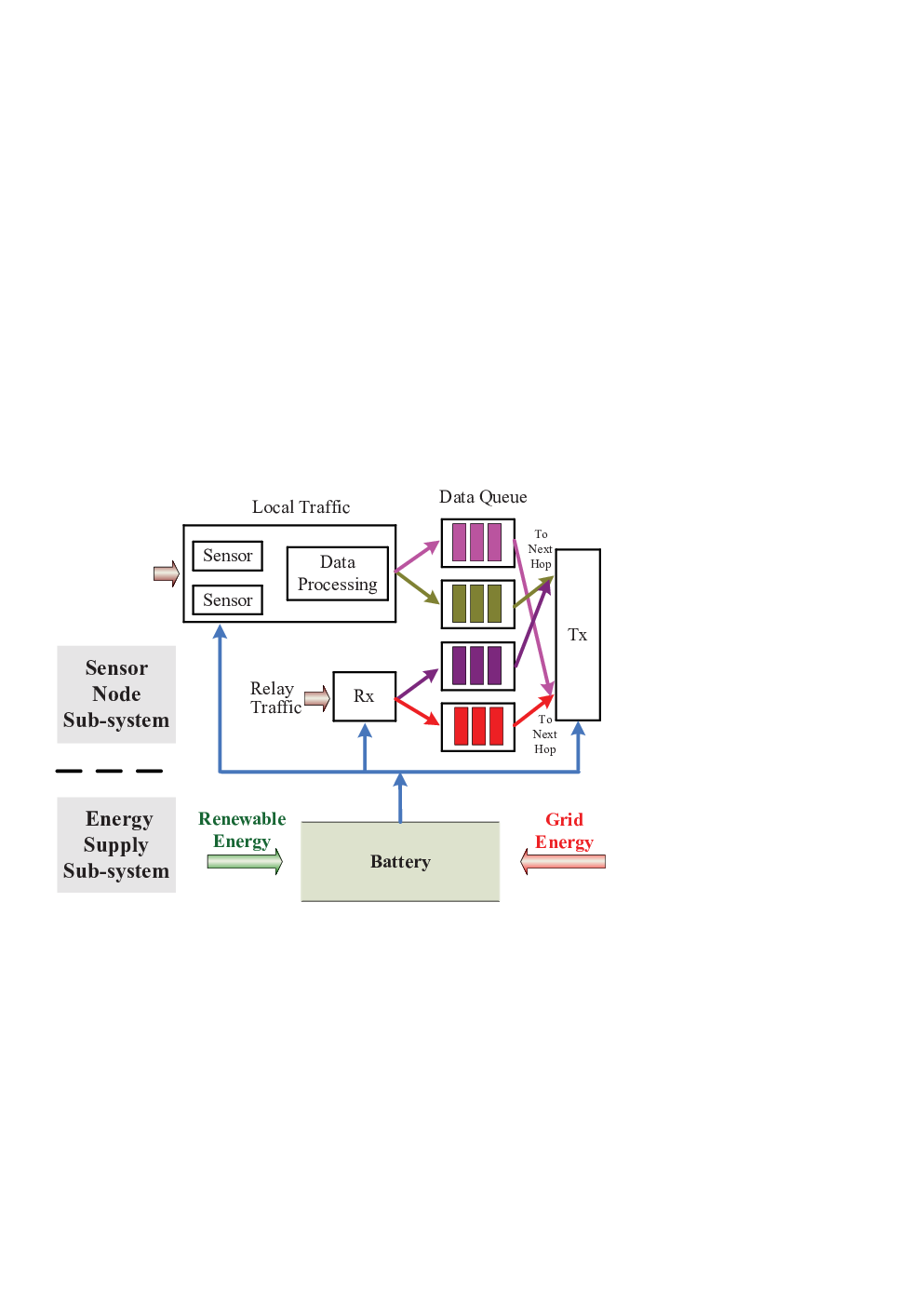
We consider a general interconnected multi-hop WSN that perfect CDMA-based medium access, and operates over time slots . WSN is modeled by a direct graph . denotes the set of sensor nodes in the network, is the set of nodes powered by EH, called EH nodes, is the set of nodes powered by EG, called EG nodes, and is the set of Mixed energy (ME) nodes powered by both EH and EG, respectively. denotes the set of all source nodes which measure the information source(s). Each source node has multiple sensor interfaces, such that it can measure multiple information sources at the same time 11 1 In the following, we use the terms information source, flow and session interchangeably. . We use to denote the set of all information sources in the network. The source node transmits the data to the corresponding destination node through multi-hop routing. represents the set of communication links. denotes the set of nodes with , and denotes the set of nodes with . Fig. 1 describes the composition of a single node system. The key notations of our system model are shown in TABLE I.
| Notation | Description |
|---|---|
| The set of sensor nodes | |
| The set of nodes powered by EH | |
| The set of nodes powered by EG | |
| The set of nodes powered by both EH and EG | |
| The set of source nodes | |
| The set of destination nodes | |
| The set of all information sessions | |
| The set of communication links | |
| The set of nodes with | |
| The set of nodes with | |
| The source rate of -th information session | |
| The transmission power of link | |
| The signal to interference plus noise ratio (SINR) of | |
| link | |
| The data transmission rate of the session over | |
| link | |
| The link capacity of link | |
| The energy consumption per data of the -th session | |
| for data sensening/processing | |
| The energy consumed when node receiving one unit | |
| data from the neighbor nodes in the network | |
| The cost per unit of electricity drawn from the electricity | |
| grid at node | |
| The total energy consumption of node | |
| The limited battery capacity of node . | |
| The harvested energy at node | |
| The energy supplied by the electricity grid at node | |
| The channel state of link | |
| The harvestable energy state of node | |
| The electricity price state at node | |
| The available amount of harvesting energy at node | |
| The energy queue size for | |
| The data backlog of the -th session at node |
II-A Source Rate and Utility
At time slot , the node measures independent parallel information sources . The measured samples of the session is compressed with rate before putting into the data queue22 2 We measure time in unit size ¡°slots,¡± for simplicity, and thus we suppress the implicit multiplication by 1 slot when converting between data rate and data amount., where denotes the source rate of the session at time slot . We assume that
| (1) |
where for all with some finite at all time. We assume that each session is associated with a utility function , which is increasing, continuously differentiable and strictly concave in with a bounded first derivative and . We use to denote the maximal first-order derivative of w.r.t. , denote .
II-B Data Transmission
We assume that the links in the network may interfere with each other when they transmit data simultaneously. We define as the transmission power allocation matrix for data transmission at slot , where is the transmission power allocated of link , and then the following inequality should be satisfied:
| (2) |
where is a finite constant to denote the maximal transmission power limitation at node .
We use to denote the signal to interference plus noise ratio (SINR) of link :
where is the noise spectral density at node , and represents the link fading coefficient from to at the slot . is the set of nodes whose transmission may interfere with the receiver of link , excluding node . We assume that may be time varying and independent and identically distributed (i.i.d.) at every slot. Denote as the network channel state matrix, taking non-negative values from a finite but arbitrarily large set .
The link capacity is defined as
Here, denotes the processing gain of the CDMA system. Note that the dependence of on and is implicit for notational convenience. Let denote the data transmission rate of the session over link , . Because of the total rates of all sessions cannot exceed the link capacity, so, . Due to the fact that is typically very large in CDMA networks, is a good approximation of , where . Thus, we make a stricter bound by the following constraint:
| (3) |
Without loss of generality, we assume that for all time over all links under any power allocation matrix and any channel state, there exists some finite constant .
II-C Energy Consumption Model
At every time slot , each node allocates power33 3 We measure time in unit size ¡°slots,¡± for simplicity, and thus we suppress the implicit multiplication by 1 slot when converting between power and energy. to accomplish its tasks, including data sensening/processing, data transmission and data reception. We define a function to denote the energy consumption of sensing/processing module for acquiring the data at a particular rate of the session at node . Inspired by [22], we also assume a linear relationship between the rate and , i.e., , where denotes the energy consumption per data of the -th session for data sensening/processing. Thus, the total energy consumption of node at slot is:
| (4) | |||||
where is the energy consumed when node receiving one unit data from the neighbor nodes in the network.
II-D Energy Supply Model
First, we describe the energy supply model of ME node shown in Fig. 1. Each ME node is equipped with a battery having the limited capacity . As depicted in Fig. 1, the harvested energy at time for ME node is stored in the battery. On the other hand, the energy supplied by the electricity grid at time for ME node is denoted with . Different from the ME node, the EH node only stores the harvested energy and the EG node only stores the energy supplied by the electricity grid.
We assume each knows its own current energy availability denoting the energy queue size for at time slot . We define over time slots as the vector of the energy queue sizes. The energy queuing dynamic equation is
| (5) | |||||
with . At any time slot , the total energy consumption at node must satisfy the following energy-availability constraint:
| (6) |
At any time slot , the total energy volume stored in battery is limited by the battery capacity, thus the following inequality must be satisfied
| (7) |
We assume the available amount of harvesting energy at slot is with for all . The amount of actually harvested energy at slot , should satisfy
| (8) |
where is randomly varying over time slots in an i.i.d. fashion according to a potentially unknown distribution and taking non-negative values from a finite but arbitrarily large set . We define the harvestable energy state .
The energy supplied by the electricity grid of the battery of node at slot should satisfy:
| (9) |
with some finite .
II-E Electricity Price Model
The cost per unit of electricity drawn from the electricity grid at node at slot is denoted by . In general, it may depend on both , the total amount of electricity from the electricity grid at slot , and an electricity price state variable , which represents such as both spatial and temporal variations, etc. For example, the per unit electricity cost may be higher during daytime, and lower at late night. We assume that is randomly varying over time slots in an i.i.d. fashion according to a potentially unknown distribution and taking non-negative values from a finite but arbitrarily large set . Denote as the electricity price vector. Similarly in [29], we assume that is a function of both and , i.e.,
Note that the dependence of on and is implicit for notational convenience in the sequel. For each given , is assumed to be a increasing and continuous convex function of . Let and denote the maximum and minimum unit electricity price in any slot in any node, respectively.
II-F Data Queue Model
For at node , we use to denote the data backlog of the -th session at time slot . We define over time slots as the data queue backlog vector. Then the data queuing dynamic equation is
| (10) | |||||
with . In any time slot , the total data output at node must satisfy the following data-availability constraint:
| (11) |
To ensure the network is strongly stable, the following inequality must be satisfied:
| (12) |
II-G Optimization Problem
The goal is to design a full distributed algorithm that achieves the optimal trade-off between the time-average utility of the source rate and the time-average cost of energy consumption in electricity grid, which subject to all of the constraints described above. Specifically, we define
| (13) | |||||
where () is a weight parameter to combine the objective functions together into a single one, and is a mapping parameter to ensure the objective functions at the same level.
Mathematically, we will address the stochastic optimization problem P1 as follows:
| (14) | |||||
| subject to |
is the set of the optimal variables of the problem P1, where , , , , are the vector of , , , , , respectively.
III Distributed Cross-layer Optimization Algorithm: EASYO
In this section, we propose an Energy mAnagement and croSs laYer Optimization algorithm (EASYO) for the problem P1. Based on the Lyapunov optimization with weight perturbation technique developed in [21], [27] and [28]44 4 The core idea of Lyapunov optimization theory can be shortly acquired from the two following linkage: ., EASYO will determine the energy harvesting, and the energy purchasing, source rate control, energy allocation for sensing/processing, transmission and reception, routing and scheduling decisions. EASYO is a fully distributed algorithm which makes greedy decisions at each time slot without requiring any statistical knowledge of the harvestable energy states, of the electricity price states and of the channel states.
III-A Lyapunov optimization
First, we introduce the weight perturbation . Note that the weight perturbation is the limited battery capacity of node defined in Section II-D. Then we define the network state at time slot as
| (15) |
Define the Lyapunov function as
| (16) |
Remark 3.1 From (16), we can see that when minimizing the Lyapunov function , the energy queue backlog is pushed towards the corresponding perturbed variable value, and the data queue backlog is pushed towards zero, which ensure the strong network stability constraint (12). Furthermore, as long as we choose appropriate perturbed variables according to (40) in Theorem 1 at the next section, the constraint (6) will always be satisfied due to (44) in Theorem 1 at the next section. Thus, we can get rid of (12) and (6) in the sequel.
Now define the drift-plus-penalty as
| (17) |
where is a non-negative weight, which can be tuned to control arbitrarily close to the optimum with a corresponding tradeoff in average queue size.
We have the following lemma regarding he upper bound of the drift-plus-penalty :
Lemma 1: Under any feasible energy management, source rate control, transmission power allocation, routing and scheduling actions that can be implemented at time , we have the upper bound of as follows
| (18) |
where
| (19) |
with , where denotes the largest number of the outgoing/incoming links that any node in the network can have. , .
is given in (20),
| (20) | |||||
where
| (21) |
| (22) |
and
| (23) |
Proof: See Appendix A.
III-B Framework of EASYO
We now present our algorithm EASYO. The main design principle of EASYO is to minimize the right hand side (RHS) of (20) subject to the constraints (1), (2), (3), (7), (8), (9) and (11).
The framework of EASYO is described in Algorithm 1 summarized in TABLE II.
| 1 Initialization: The perturbed variables and the penalty parameter is given. 2 Repeat at each time slot : 3 Observe ; 4 Choose the set of the optimal variables as the optimal solution to the following optimization problem P2: subject to 5 Update the energy queues and data queues according to (5) and (10), respectively. |
Remark 3.2 Note that the algorithm EASYO only requires the knowledge of the instant values of . It does not require any knowledge of the statistics of these stochastic processes. The remaining challenge is to solve the problem P2, which is discussed below.
III-C Components of EASYO
At each time slot , after observing , all components of EASYO is iteratively implemented in distributed manner to cooperatively solve the problem P2. Next, we describe each component of EASYO in detail.
(1) Energy Management For each node , combining the first term of the RHS of (20) with the the constraint (7), (8) and (9), we have the optimization problem of and as follows:
| subject to | (24) | ||||
| (25) | |||||
| (26) |
Remark 3.3 Energy management component is composed of energy harvesting and energy purchasing. Furthermore, since is increasing and continuous convex on for each , it is easy to verify that energy management component is a convex optimization problem in , which can be solved efficiently.
Remark 3.4 From (26), we can see that all the incoming energy is stored if there is enough room in the energy buffer according to the limitation imposed by , and otherwise it stores all the energy that it can, filling up the battery size of . Hence, for all , which means that EASYO can be implemented with finite energy storage capacity at node .
(2) Source Rate Control For each session at source node , combining the second term of the RHS of (20) with the constraint (1), we have the optimization problem of as follows:
| subject to | (27) |
Let be the unique maximizer. By the Kuhn-Tucker theorem, is given by
| (28) |
where , is the inverse of the derivative of .
(3) Joint Optimal Transmission Power Allocation, Routing and Scheduling Combining the third term of the RHS of (20) with the constraints (2), (3) and the data-availability constraint (11), we have the optimization problem of and as follows:
| subject to | ||||
| (29) |
Now, we will solve the optimization problem (29). Define the weight of the session over link as:
| (30) |
where
| (31) |
denotes the data amount of the session which the node can receive at most at time slot .
Transmission Power Allocation Component For each node , find any . Define as the corresponding optimal weight of link . Observe the current channel state , and select the transmission powers by solving the following optimization problem:
| subject to | (32) |
Routing and Scheduling Component The data of session is selected for routing over link whenever . That is, if , set .
Remark 3.5: If we set , the joint transmission power allocation, routing and scheduling component is to minimize the third term of the RHS in (20). Inspired by [27] and [28], we set a non-zero in (30), leading to a easy way to determine the upper bound of all queue sizes shown in Theorem 1. Also the definition (31) of can ensure the constraints (11) will always be satisfied. The detailed proof will be given in Theorem 1. Thus, we can get rid of this constraint (11) in (32).
Remark 3.6: Our proposed EASYO is designed to minimize the RHS of (20). Each component contributes to minimizing the part of the RHS of (20). Taking all components together, EASYO contributes to minimize the whole RHS of (20), and thus to minimize . Because the whole RHS of (20) incorporates the Lyapunov drift, EASYO is stable. Meanwhile, since it also incorporates the objective of the problem P1, EASYO is optimal.
Remark 3.7: The former two components of EASYO are computed in closed form or numerically solved through a simple convex optimization problem, only based on the local information. The unique challenge of distributed implementation of EASYO is to distributedly solve the transmission power allocation problem (32). Next, we will develop the distributed algorithm.
III-D Distributed Implementation of Transmission Power Allocation
After implementing a variable change , and taking the logarithm of both sides of the constraint in problem (32), the problem (32) can be equivalently transformed into the problem P3
| s.t. | (33) |
where , is defined in (34).
| (34) | ||||
It is not difficult to prove that is a strictly concave function of a logarithmically transformed power vector [30]. Due to (7) or (26), we have , so , thus is a strictly concave function of . To sum up, the objective of P3 is a strictly convex in . Furthermore, since is a strictly concave in , P3 is a strictly convex optimization problem, which has the global optimum.
To distributedly solve P3, we propose a distributed iterative algorithm based on block coordinate descent (BCD) method whereby, at every iteration, a single block of variables is optimized while the remaining blocks are held fixed. More specifically, at iteration , which represents the -th iteration at the time slot , for each node , the blocks are updated through solving the following optimization problem (35), where are held fixed.
| subject to | (35) |
The global rate of convergence for BCD-type algorithm has been studied extensively when the block variables are updated in both the classic Gauss-Seidel fashion and the randomized update rule[31][32]. Since the optimization problem P3 is strongly convex in , our proposed BCD-based distributed iterative algorithm can converge to the global optimum of P3.
IV Performance analysis
Now, we analyze the performance of our proposed algorithm EASYO. To start with, we assume that there exists such that
| (36) |
Theorem 1: Implementing the algorithm EASYO with any fixed parameter for all time slots, we have the following performance guarantees:
(A). Suppose the initial data queues and the initial energy queues satisfy:
| (37) | |||||
| (38) |
where the queue upper bounds are given as follows:
| (39) |
| (40) |
Then, the data queues and the energy queues of all nodes for all time slots are always bounded as
| (41) | |||||
| (42) |
(B). The objective function value of the problem P1 achieved by the proposed algorithm EASYO satisfies the bound
| (43) |
where is the optimal value of the problem P1, and .
(C). When node allocates nonzero power for data sensing, data transmission and/or data reception, we have:
| (44) |
(D). For node , when any data of the -th session is transmitted to other node, we have:
| (45) |
Proof: Please see Appendix B-E.
Remark 4.1: Theorem 1 shows that a control parameter enables an explicit trade-off between the average objective value and queue backlog. Specifically, for any , the proposed distributed algorithm EASYO can achieve a time average objective that is within of the optimal objective shown in (43), while ensuring that the average data and energy queues have upper bounds of shown in (41) and (42), respectively. In the section V, the simulations will verify the theoretic claims.
V Simulation Results
In this section, we provide the simulation results of the algorithm EASYO for the network scenario shown in Fig.2. In this scenario, we consider a multi-channel WSN with 20 nodes, 78 links, 6 sessions transmitted on 14 different channels. Throughout, the form of the rate utility function is set as , so . The form of the electricity cost function is set as .

Set several default values as follows: ; ; ; ; , , . We set all the initial queue sizes to be zero.
The channel-state matrix has independent entries that for every link are uniformly distributed with interval , , as default values and denotes the distance between transmitter and receiver of the link, while the energy-harvesting vector has independent entries that are uniformly distributed in , with as default value. The electricity price vector has independent entries that are uniformly distributed in with , as default values, so , . All statistics of , and are i.i.d. across time-slots.
We simulate =[100,300,500,700,1000,1500]. In all simulations, the simulation time is time slots. The simulation results are depicted in Fig. 3. From Fig. 3 (a), we see that as increases, the time average optimization objective value keep increasing and converge to very close to the optimum. This confirms the results of (43). From Fig. 3 (b), we see that as increases, the average data queue length keeps increasing. From Fig. 3 (c)-(e), we observe that the battery queue size increases as increases. A closer inspection of the results also reveals a linear increase of the time average data and energy queue size with respect to . This shows a good match between the simulations and Theorem 1.


For better verification of the queueing bounds, we also present the data queue process of node for session , of node for session and of node for session under in Fig 4(a), and the energy queue processes for EH node , for EG node and for ME node under in Fig. 4(b)-(d), respectively. It can be verify that all queue sizes can quickly converge with the upper bound given in Theorem 1.
Transmission power allocation problem P3 is the most complex component in our proposed EASYO. We proposed a BCD-based distributed iterative algorithm to solve the problem P3. During the implementation of EASYO, we catch four different snapshots of the iterative procedure of BCD-based algorithm, shown in Fig. 5. From Fig. 5, we can see that BCD-based algorithm can quickly converge to the global optimum. Thus, our proposed EASYO is a low-complexity distributed algorithm.

Next, we investigate the impacts of a variety of system parameters on the objective value, rate utility and electricity cost. Fig. 6 shows the impact of the node power supply manner and the maximum available harvested energy on the objective value. From Fig. 6, we can see that the lowest objective value is achieved at all EH nodes scenario with much smaller than and the highest objective value is achieved at all EH nodes scenario with equal to . Due to the expense of the highest energy cost, all EG nodes scenario achieves the objective value lower than all EH nodes scenario or default node scenario with . In contrast, all EG nodes scenario achieves the objective value higher than all EH nodes scenario or default node scenario with , which results in the low energy supply and low data transmission.

We investigate the impact of the electricity price on the rate utility and energy cost. We set three different electricity prices as , and , respectively. Fig. 7 shows that the electricity cost increases along with the increase of the electricity price. In order to reduce the electricity cost, EASYO reduce the energy consumption, and thus the corresponding rate utility decreases.

We investigate the impact of the weight parameter on the rate utility and energy cost. We set three the weight parameters as , and , respectively. When the weight parameter is chosen as a large value, EASYO focuses on the rate utility maximization rather than the electricity cost minimization. The results of Fig. 8 verify this situation, where the rate utility increases and the electricity cost also increases under a large value .

Fig. 9 shows the impact of on the rate utility and energy cost. The larger , the more energy is required to supply for data sensing/processing, leading to the less energy used in data transmission, and the lower rate utility.
VI Conclusions
Because of the instable energy supply and the limited battery capacity in EH node, it is very difficult to ensure the perpetual operation for WSN. In this paper, we consider heterogeneous energy supplies from renewable energy and electricity grid, multiple energy consumptions and multi-dimension stochastic natures in the system model, and formulate a discrete-time stochastic cross-layer optimization problem to optimize the trade-off between the time-average rate utility and electricity cost. To the end, we propose a fully distributed and low-complexity cross-layer algorithm only requiring knowledge of the instantaneous system state. The theoretic proof and the extensive simulation show that a parameter enables an explicit trade-off between the optimization objective and queue backlog. In the future, we are interested in two aspects of delay reduction by utilizing the shortest path concept, and by modifying the queueing disciplines.
Appendix A Proof of Lemma 1
| (46) |
| (47) |
| (48) | |||||
Appendix B Proof of Part (A) in Theorem 1
For , we can easily have (41), then we assume (41) is hold at time slot , next we will show that it holds at .
Case 1: If node doesn’t receive any data at time , we have .
Case 2: If node receives the endogenous data from other nodes , we can get from (30) that . By plugging (23) and (31), we have . Then, . Due to and , we have
| (49) |
Plugging (41) into (49), we have
| (50) | |||||
At every slot, the node can receive the amount of data at most . So
| (51) |
Case 3: If node only receives the new local data, according to (27), the optimal value will met , where denotes the first derivative of . So we have , and then . At every time, the new local data received at most is , so, .
To sum up the above, we complete the proof of (41).
From Remark 3.5 we can have (42).
Appendix C Proof of Part (B) in Theorem 1
The proof procedure of Part (B) in Theorem 1 is similar to that in [20], and hence is omitted for brevity.
Appendix D Proof of Part (C) in Theorem 1
It is easy to verify that the following inequality holds according to the definition of :
| (52) |
where obtained by setting of to zero, and .
By plugging (31) and (41) into (53), we have
| (54) | |||||
Since (54) holds for any session through link , we have
| (55) |
We assume that , when node allocates nonzero power for data sensing, compression and transmission. Furthermore, we assume that the power allocation control vector is the optimal solution to (32), and without loss of generality, there exists some . By setting in , we get another power allocation control vector . We denote as the objective function of (32). In this way, we get:
| (56) |
From (52), we have for . So
| (57) |
According to our assumption and the definition of in (40), we have
| (58) |
Plugging (36), (55) and (58) into (57), we have
Appendix E Proof of Part (D) in Theorem 1
References
- [1] I. F. Akyildiz, W. Su, Y. Sankarasubramaniam, and E. Cayirci, “Wireless Sensor Networks: A Survey”, Computer Networks (Elsevier) , vol. 38, no. 4, pp. 393-422, March 2002.
- [2] W. Xu, Q. Shi, X. Wei, Z. Ma, X. Zhu, and Y. Wang, “Distributed Optimal Rate-Reliability-Lifetime Tradeoff in Time-Varying Wireless Sensor Networks”, IEEE Transactions on Wireless Communications, vol. 13, no. 9, pp. 4836-4847, 2014.
- [3] J. Chen, W. Xu, S. He, Y. Sun, P. Thulasiraman and X. Shen, “Utility-Based Asynchronous Flow Control Algorithm for Wireless Sensor Networks”, IEEE Journal on Selected Areas in Communications, vol. 28, no. 7, pp. 1116-1126, 2010.
- [4] S. Sudevalayam and P. Kulkarni, “Energy harvesting sensor nodes: Survey and implications”, IEEE Communications Surveys and Tutorials, vol. 13, no. 3, pp. 443-461, 2011.
- [5] S. He, J. Chen, F. Jiang, D. Yau, G. Xing and Y. Sun, “Energy Provisioning in Wireless Rechargeable Sensor Networks”, IEEE Transactions on Mobile Computing, vol.12, no. 10, pp. 1931-1942, Oct. 2013.
- [6] H. Ju and R. Zhang, “Throughput maximization in wireless powered communication networks”, IEEE Transactions on Wireless Communications, vol. 13, no. 1, pp. 418-428, January, 2014.
- [7] V. Sharma, U. Mukherji, V. Joseph, and S. Gupta, “Optimal energy management policies for energy harvesting sensor nodes,” IEEE Transactions Wireless Communications, vol. 9, no. 4, pp. 1326-1336, Apr. 2010.
- [8] K. Tutuncuoglu, A. Yener, “Optimum Transmission Policies for Battery Limited Energy Harvesting Nodes”, IEEE Transactions on Wireless Communications, vol. 11, no. 3, pp.1180-1189, 2012.
- [9] O. Ozel, K. Tutuncuoglu, J. Yang, S. Ulukus, and A. Yener, “Transmission with energy harvesting nodes in fading wireless channels: Optimal policies”, IEEE Journal on Selected Areas in Communications, vol. 29, no. 8, pp. 1732-1743, Sep. 2011.
- [10] R. Srivastava and C. E. Koksal, “Basic performance limits and tradeoffs in energy harvesting sensor nodes with finite data and energy storage”, IEEE/ACM Transactions on Networking, vol. 21, no. 4, pp. 1049-1062, Aug. 2013.
- [11] P. Castiglione, O. Simeone, E. Erkip, and T. Zemen, “Energy management policies for energy-neutral source-channel coding”, IEEE Transactions on Communications, vol. 60, no. 9, pp. 2668-2678, Sep. 2012.
- [12] Y. Zhang, S. He, J. Chen, Y. Sun, X. Shen, “Distributed Sampling Rate Control for Rechargeable Sensor Nodes with Limited Battery Capacity”, IEEE Transactions on Wireless Communications, vol. 12, no. 6, pp. 3096-3106, 2013
- [13] S. Mao, M. Cheung, V. Wong, “Joint Energy Allocation for Sensing and Transmission in Rechargeable Wireless Sensor Networks”, IEEE Transactions on Vehicular Technology, vol. 63, no. 6, pp. 2862-2875, 2014.
- [14] K. Fan, R. Liu, Z. Zheng, and P. Sinha, “Perpetual and Fair Data Collection for Environmental Energy Harvesting Sensor Networks”, IEEE/ACM Transactions on Networking, vol. 19, no. 4, pp947-960, 2011.
- [15] Z. Mao, C. E. Koksal, and N. B. Shroff, “Near optimal power and rate control of multi-hop sensor networks with energy replenishment: Basic limitations with finite energy and data storage”, IEEE Transactions on Automatic Control, vol. 57, no. 4, pp. 815-829, Apr. 2012.
- [16] S. Chen, P. Sinha, N. Shroff, and C. Joo, “A simple asymptotically optimal energy allocation and routing scheme in rechargeable sensor networks”, in Proc. of IEEE INFOCOM 2012, Orlando, FL, USA, Mar. 2012.
- [17] S. Sarkar, M.H.R. Khouzani, and K. Kar, “Optimal Routing and Scheduling in Multihop Wireless Renewable Energy Networks”, IEEE Transactions on Automatic Control, vol. 58, no. 7, pp. 1792-1798, 2013.
- [18] W. Xu, S. Wen, Q. Shi, J. Wu, Y. Wang, “Distributed Event-Triggered Flow Control for Utility Fairness in Energy Harvesting Wireless Sensor Networks”, International Journal of Sensor Networks, to appear.
- [19] M. Gatzianas, L. Georgiadis, and L. Tassiulas, “Control of wireless networks with rechargeable batteries”, IEEE Transactions on Wireless Communications, vol. 9, no. 2, pp. 581-593, Feb. 2010.
- [20] L. Huang and M. J. Neely, “Utility optimal scheduling in energy harvesting networks”, IEEE/ACM Transactions on Networking, vol. 21, no. 4, pp. 1117-1130, Aug. 2013.
- [21] L. Huang and M. J. Neely, “Utility optimal scheduling in processing networks”, Performance Evaluation (Elsevier), vol. 68, no. 11, pp. 1002-1021, Nov. 2011.
- [22] C. Tapparello, O. Simeone, M. Rossi, “Dynamic Compression-Transmission for Energy-Harvesting Multihop Networks With Correlated Sources”, IEEE/ACM Transactions on Networking, Digital Object Identifier: 10.1109/TNET.2013.2283071
- [23] C. B. Margi, V. Petkov, K. Obraczka, R. Manduchi, “Characterizing energy consumption in a visual sensor network testbed”, in Proc. of TridentCom 2006, Barcelona, Spain, March 2006.
- [24] X. Liu, O. Simeone, E. Erkip, “Energy efficient sensing and communication of parallel sources”, IEEE Transactions on Communications, vol. 60, no. 12, pp. 3826-3835, December 2012.
- [25] H. Huang, V. K. N. Lau, “Decentralized Delay Optimal Control for Interference Networks With Limited Renewable Energy Storage”, IEEE Transactions on Signal Processing, vol. 60, no. 5, pp. 2552-2561, May 2012.
- [26] J. Gong, S. Zhou, Z. Niu, “Optimal Power Allocation for Energy Harvesting and Power Grid Coexisting Wireless Communication Systems”, IEEE Transactions on Communications, vol. 61, no.7, pp. 3040-3049, 2013.
- [27] M. J. Neely, “Stochastic Network Optimization with Application to Communication and Queueing Systems”, Synthesis Lectures on Communication Networks, Morgan & Claypool, 2010.
- [28] L. Georgiadis, M.J. Neely, L. Tassiulas, “Resource allocation and cross-layer control in wireless networks”, Foundations and Trends in Networking, vol. 1, no. 1, pp. 1-144, 2006
- [29] R. Urgaonkar, B. Urgaonkar, M. J. Neely and A. Sivasubramaniam, “Optimal Power Cost Management Using Stored Energy in Data Centers”, in Proc. ACM SIGMETRICS 2011, San Jose, CA, USA. June 2011.
- [30] S. Boyd and L. Vandenberghe, “Convex Optimization”, Cambridge, U.K.: Cambridge University Press, 2004.
- [31] M. Hong, X. Wang, M. Razaviyayn, and Z-Q. Luo, “Iteration complexity analysis of block coordinate descent methods”, Technical report, University of Minnesota, USA, 2013. http://arxiv.org/abs/1310.6957.
- [32] A. Beck and L. Tetruashvili, “On the convergence of block coordinate descent type methods”, SIAM Journal on Optimization, vol. 23, no.4, pp.2037-2060, 2013.
- [33] D. P. Bertsekas, A. Nedic¡ä, and A. E. Ozdaglar, “Convex Analysis and Optimization”, Belmont, MA: Athena Scientific, 2003.