A regression tree approach to identifying subgroups
with differential treatment effects
Abstract
In the fight against hard-to-treat diseases such as cancer, it is often difficult to discover new treatments that benefit all subjects. For regulatory agency approval, it is more practical to identify subgroups of subjects for whom the treatment has an enhanced effect. Regression trees are natural for this task because they partition the data space. We briefly review existing regression tree algorithms. Then we introduce three new ones that are practically free of selection bias and are applicable to two or more treatments, censored response variables, and missing values in the predictor variables. The algorithms extend the GUIDE approach by using three key ideas: (i) treatment as a linear predictor, (ii) chi-squared tests to detect residual patterns and lack of fit, and (iii) proportional hazards modeling via Poisson regression. Importance scores with thresholds for identifying influential variables are obtained as by-products. And a bootstrap technique is used to construct confidence intervals for the treatment effects in each node. Real and simulated data are used to compare the methods.
Key words: Missing values; proportional hazards; selection bias.
1 Introduction
For many diseases, such as cancer, it is often difficult to find a treatment that benefits all patients. Current thinking in drug development is to find a subject subgroup, defined by individual characteristics, that shows a large treatment effect. Conversely, if a treatment is costly or has potential negative side effects, there is interest to look for subgroups for which it treatment is ineffective. This problem of searching for subgroups with differential treatment effects is known as subgroup identification [9, 13, 20].
To fix ideas, suppose for the moment that the response variable is uncensored and the treatment variable takes values . Let denote a vector of covariates. Given a subgroup defined in terms of , let denote the effect size of . The goal is to find the maximal subgroup with the largest value of , where the size of is measured in terms of its probability of occurrence . If is subject to censoring, we replace the mean of by the log-hazard rate so that is the largest absolute log-hazard ratio between any two treatments.
Consider, for example, data from a randomized trial of the German Breast Cancer Study Group [30, 27] with 686 subjects where the response is recurrence-free survival time in days. The trial was designed as a factorial comparing 3 vs. 6 cycles of chemotherapy and presence vs. absence of hormone therapy (Tamoxifen). The breast cancer data contain, however, no information on the number of cycles of chemotherapy, presumably because it was previously found not significant [31]. Median follow-up time was nearly 5 years and 387 subjects did not experience a recurrence of the disease during the trial (54 percent censoring). The variables are hormone therapy (horTh: yes, no), age (21–80 years), tumor size (tsize: 3–120 mm), number of positive lymph nodes (pnodes: 1–51), progesterone receptor status (progrec: 0–2380 fmol), estrogen receptor status (estrec: 0–1144 fmol), menopausal status (menostat: pre, post), and tumor grade (tgrade: 1, 2, 3). A standard proportional hazards regression model shows that hormone therapy has a significant positive effect on survival, with and without adjusting for the covariates [29, 12]. Since hormone therapy has side effects and incurs extra cost, it is useful to find a subgroup where the treatment has little effect.
Parametric and semi-parametric models such as the proportional hazards model do not easily lend themselves to this problem. Besides, if there are more variables than observations, such as in genetic data, these models cannot be used without prior variable selection. Regression tree models are better alternatives, because they are nonparametric, naturally define subgroups, scale with the complexity of the data, and are not limited by the number of predictor variables.
Following medical practice [15], we call a variable prognostic if it provides information about the response distribution of an untreated subject. That is, it has marginal effects on the response but does not interact with treatment. Examples are age, family history of disease, and prior therapy. A variable is predictive if it defines subgroups of subjects who are more likely to respond to a given treatment. That is, it has interaction effects with the treatment variable. Figure 1 shows two regression tree models and the Kaplan-Meier curves in the terminal nodes of the trees. In the Gs model on the left, variable pnodes is prognostic: recurrence probability is reduced if pnodes 3, with and without treatment. In the Gi model on the right, variable progrec is predictive: hormone therapy has little effect if progrec 21 and an enhanced effect otherwise.
pstreeTC [tnpos=l]pnodes 3 [tnpos=a]Gs
TC[fillcolor=cyan,fillstyle=solid] (0.33, 1.02)
[tnpos=l]370
TC[fillcolor=cyan,fillstyle=solid] (0.46, 1.06)
[tnpos=r]302
pstreeTC [tnpos=l]progrec 21 [tnpos=a]Gi
TC[fillcolor=cyan,fillstyle=solid]
(0.55, 1.42) [tnpos=l]274
TC[fillcolor=cyan,fillstyle=solid] (0.29, 0.94)
[tnpos=r]398

The main goal of this article is to introduce the algorithms that yield the models in Figure 1 and to compare them against existing solutions, which are briefly reviewed in Sec. 2. Sec. 3 presents the new algorithms for uncensored response variables. Sec. 4 compares the selection bias and accuracy of the new and old methods and Sec. 5 proposes a bootstrap technique for computing confidence intervals of treatment and other effects in the subgroups. Sec. 6 extends the algorithms to censored survival data and Sec. 7 obtains importance scores for ranking the variables and and thresholds for identifying the unimportant ones. Sec. 8 gives an application to a retrospective candidate gene study where there are large numbers of missing values and Sec. 9 concludes the article with some closing remarks.
2 Previous work
Let and denote the survival time and covariate vector of subject . Let be an independent observation from some censoring distribution and let be the event indicator. The observed data vector of subject is , where , . Let denote the hazard function at . The proportional hazards model specifies that , where is a baseline hazard and is a linear function of the covariates.
Assuming that the treatment has two levels (denoted by ), one approach [26] splits each node into left and right child nodes and to maximize the Cox partial likelihood ratio statistic for testing against . A related approach, called interaction trees (IT) [33], chooses the split that minimizes the p-value from testing in the model . If there is no censoring, the model is . Both methods employ the greedy search paradigm of evaluating all splits and on every and every , where is a half line if is ordinal and is a subset of values if is categorical. As a result, they are computationally expensive and biased toward selecting variables that allow more splits. Further, because is a function of and hence of , the tree models do not have proportional hazards and regression coefficients in different nodes cannot be compared.
The virtual twins (VT) method [13] is restricted to binary variables . It first generates a random forest [5] model to estimate the treatment effect of each subject, using as split variables , with categorical variables converted first to dummy 0-1 variables. Then it uses RPART [34] to construct a classification or regression tree model to predict for each subject and to obtain the subgroups. If a classification tree is used, the two classes are defined by the estimated being greater or less than a pre-specified constant; if a regression tree is used, the subgroups are the terminal nodes with estimated greater than a pre-specified constant. Although the basic concept is independent of random forest and RPART, their use gives VT all their weaknesses, such as variable selection bias and (with random forest) lack of a preferred way to deal with missing values. Further, VT is limited to binary and .
The subgroup identification based on differential effect search (SIDES) method [20] finds multiple alternative subgroups by identifying the best five (default) splits of each node that yield the most improvement in a desired criterion, such as the p-values of the differential treatment effects between the two child nodes, the treatment effect size in at least one child node, or the difference in efficacy and safety between the two child nodes. For each split, the procedure is repeated on the child node with the larger improvement. Heuristic and resampling-based adjustments are applied to the p-values to control for multiplicity of splits and correlations among the p-values. The method appears to be most useful for generating candidate subgroups with large differential effects, but because only variables that have not been previously chosen are considered for splitting each node, the method may not be effective if the real subgroups are defined in terms of interval sets of the form . The current implementation is limited to treatments with two levels.
Most methods can control the minimum node sample size so that the subgroups have sufficient numbers of observations. The qualitative interaction tree (QUINT) method [11] deals with this directly by optimizing a weighted sum of a measure of effect size and a measure of subgroup size. It looks for “qualitative interactions,” where one treatment performs better than another in one subgroup and worse in another subgroup. Similar to the above methods, QUINT finds the subgroups by searching over all possible splits on all predictor variables. Its current implementation is limited to ordinal , uncensored , and binary .
3 Uncensored data
By evaluating all possible splits on all variables to optimize an objective function, each method (except possibly for SIDES) is biased toward selecting variables that allow more splits. This is due to an ordinal variable with unique values yielding splits and a categorical variable with the same number of unique values yielding splits. As a result, a variable that allows many splits has a greater chance to be selected than one with few splits. Besides increasing the chance of spurious splits, the bias can undermine the credibility of the results. SIDES tries to control the bias with Bonferroni-type adjustments, but this can lead to over correction, as in the CHAID [16] classification tree algorithm, which is biased toward selecting variables with few splits.
The GUIDE algorithm [21, 23] overcomes this problem by using a two-step approach to split selection: first find the split variable and then search for the best split on the selected variable. The first step yields substantial computational savings, because there is no need to find the best splits on the all the other variables. It also eliminates selection bias, at least in principle, by using chi-squared tests to select the split variable. QUEST [25], CRUISE [17], and CTREE [14] are other algorithms that employ significance tests for variable selection. In this section we extend GUIDE to subgroup identification for the case where is not censored.
3.1 Gc: classification tree approach
This method requires that and are binary, taking values, 0, and 1, say. Then a classification tree may be used to find subgroups by defining the class variable as :
This is motivated by the observation that the subjects for which respond differentially to treatment and those for which do not. Thus a classification tree constructed with as the response variable will likely identify subgroups with differential treatment effects. Although any classification tree algorithm may be used, we use GUIDE [23] here because it does not have selection bias, and call it the Gc method (“c” for classification).
3.2 Gs and Gi: regression tree approach

resid 0 21 6 resid 0 2 21 , resid 0 1 21 resid 0 26 2 ,
The GUIDE linear regression tree algorithm [21] provides an alternative approach that permits and to take more than two values. At each node, we fit a model linear in and select the variable to split it by examining the residual patterns for each level of . Consider, for example, data generated from the model
| (1) |
where and is independent normal. Because the true subgroup is , we should split the data using . Figure 2 shows how this conclusion can be reached from the data alone. The top row plots and the residuals vs. , where the residuals are from fitting the model . The middle row plots residuals vs. for each level. The distinct nonrandom patterns in the latter plots are indicators that has an interaction with . No other variables can be expected to show such strong patterns. We measure the strength of the interaction by forming a contingency table with the residual signs as rows and grouped values of (obtained by dividing its values at the sample mean) as shown in the bottom row of the figure, computing a chi-squared statistic for each level of , and summing them. Repeating this procedure for each , we rank the variables and select the one with the largest summed chi-squared to split the data. We call this the Gs method (“s” for sum).
Contingency table tests are convenient because they are quick to compute, can detect a large variety of patterns, and are applicable to categorical variables, where we use their values for the columns. Because the latter changes the degrees of freedom (df) of the chi-squared statistics, we need to adjust for differences in df before summing them. We do this by following GUIDE which uses a double application of the Wilson-Hilferty approximation [35] to convert each contingency table chi-squared statistic to a 1-df chi-squared quantile. Specifically, let and be chi-squared quantiles with df and , respectively, degrees of freedom. Then (see [23])
| (2) |
After a variable is selected, a search is carried out for the best split on the variable that minimizes the sum of squared residuals in the two child nodes and the process is applied recursively to each node. The detailed algorithm, including handling of missing values, is given below.
Algorithm 1
Gs split selection.
- 1.
Fit the least squares model to the data in the node and compute the residuals. Let denote the set of observations with in the node.
- 2.
For each and .
- (a)
Form a contingency table from the data in using the signs (positive vs. non-positive) of the residuals as columns and the (grouped) values as rows. If is ordinal, divide its values into two groups at the mean. Otherwise, if is categorical, let its values define the groups. If there are missing values, add an additional “missing value” group.
- (b)
Compute the chi-squared statistic for testing independence, and let denote its degrees of freedom. Use (2) to convert to the 1-df chi-squared quantile
- (a)
- 3.
Treating as a chi-squared variable with df, use (2) a second time to convert it to a 1-df chi-squared quantile
- 4.
Let be the variable with the largest value of .
- (a)
If is ordinal, let denote the event that is missing (if any) and its complement. Then search through the values of for the split or that minimizes the sum of the squared residuals fitted to the two child nodes produced by the split.
- (b)
If is categorical, let denote its number of categories (including the missing category, if any). If , search over all splits of the form to find the one that minimizes the sum of squared residuals in the two child nodes. If , limit the search to splits as follows.
- i.
Label an observation as belonging to class 1 if it has a positive residual and as class 2 otherwise.
- ii.
Order the values by their proportions of class 1 subjects in the node.
- iii.
Select the split along the ordered values that yields the greatest reduction in the sum of Gini indices. (This mimics a technique in [6, p. 101] for piecewise constant least-squares regression.)
- i.
If there are no missing values in the training data, future cases missing are sent to the more populous child node.
- (a)
Because Gs (as well as MOB) is sensitive to both prognostic and predictive variables, it may be ineffective if only subgroups defined by predictive variables are desired. To see this, suppose now that the data are generated from the true model
| (3) |
with independent normal. The simulated data plots in Figure 3 show that Gs will choose with high probability even though it is prognostic but not predictive. IT overcomes this by adding the interaction to the fitted model and testing for its significance, but this approach requires searching over the values of , which produces selection bias and may be impractical if takes more than two levels. To get around these problems, we instead test for lack of fit of the model
| (4) |
where if it is categorical and is the indicator function with being the sample mean of at the node otherwise. Then we select the most significant to split the data. Turning an ordinal into a binary variable may lead to loss of power, but this is compensated by increased sensitivity to interactions of all kinds, including those that cannot be represented by cross-products of indicators. We call this the Gi method (“i” for interaction). The procedure, including handling of missing values, is given next.

Algorithm 2
Gi split selection.
- 1.
For each variable at each node:
- (a)
If is ordinal, divide its values into two groups at its mean. If is categorical, let its values define the groups. Add a group for missing values if there are any. Let denote the factor variable created from the groups.
- (b)
Carry out a lack-of-fit test of the model (4) on the data in the node and convert its p-value to a 1 df chi-squared statistic .
- (a)
- 2.
4 Bias and accuracy
4.1 Selection bias
It is obviously important for a tree model not to have selection bias if it is used for subgroup identification. At the minimum, this requires that if all the variables are independent of , each has the same probability of being selected to split each node. We carried out a simulation experiment to compare the methods on this score. The experiment employed two predictors, and , and Bernoulli response and treatment variables and each with success probability 0.50. All variables are mutually independent. The distributions of and ranged from standard normal, uniform on the integers 1, 2, 3, 4, and equi-probable categorical with 3 and 7 levels, as shown in Table 2.
Based on a sample size of 100 for each iteration, Figure 4 shows the frequency that each method selects to split the root node over 2500 simulation iterations. Simulation standard errors are less than 0.01. An unbiased method should select or with equal probability regardless of their distributions. The results show that IT, QUINT, SIDES and VT have substantial selection biases (QUINT is limited to ordinal ). IT and QUINT are biased towards selecting the variable that has more splits while SIDES and VT are opposite. In contrast, the selection frequencies of Gs and Gc are all within three simulation standard errors. The frequencies of Gi are also within three standard errors, except when is categorical with 7 levels where it has a slightly higher chance to be selected.

4.2 Accuracy
We use three simulation models to compare the methods in terms of their accuracy in selecting the correct variables and the correct subgroups. Each model employs a binary treatment variable with and 100 variables , all mutually independent. Each takes categorical values 0, 1, or 2 (simulating genetic markers with genotypes AA, Aa, and aa), with and having identical marginal distribution , and . The others have marginal distributions , and , with () being independently simulated from a beta distribution with density . The models for are:
Figure 5 shows the values of for models M1 and M3. Variables and are predictive in M1 but prognostic in M3. Figure 6 shows the values for model M2 which is more complex; and are predictive and and are prognostic. M2 tests the ability of a method to distinguish between the two variable types.


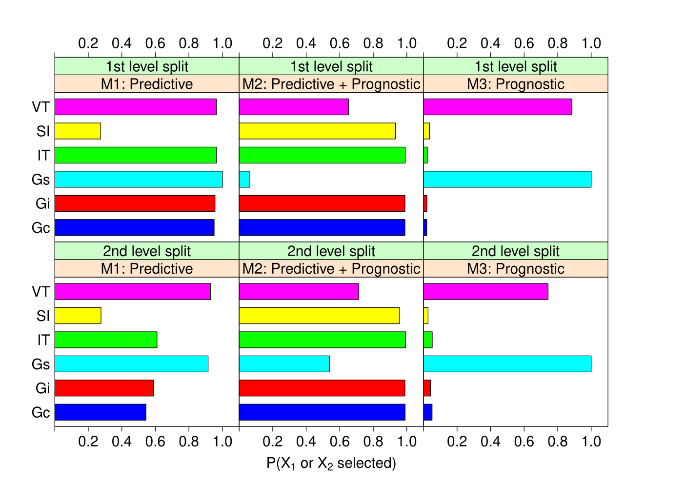
First we compare the frequencies that and are chosen at the first two levels of splits of a tree. For each of 1000 simulation iterations, 100 observations of the vector are simulated from each model and a tree is constructed using each method. The frequencies that or is selected to split the root node (1st level split) as well as one or both of its child nodes (2nd level split) are graphed in Figure 7. QUINT is excluded because it does not allow categorical variables and the models do not have qualitative interactions. For model M1, where and are predictive and there is no other variable associated with , all but SIDES select or to split the root node with comparably high frequency. At the second split level, the frequencies for Gs and VT are distinctly higher than those for Gc, Gi and IT, while that for SIDES remains low. Therefore Gs and VT are best and Gc, Gi and IT second best for model M1 on this criterion. The situation is different in M2 which has two predictive and two prognostic variables. Now Gc, Gi, IT and SIDES are best and Gs is worst and VT second worst. This shows that Gs and VT have difficulty distinguishing between predictive and prognostic variables. This behavior is repeated in M3 which has no predictive variables. Here the probability that or is selected to split the nodes should not be different from that of the other 98 variables, but Gs and VT continue to pick the former with high frequencies. Only Gc, Gi, IT, and SIDES perform correctly in this case.
Next we compare the power of the methods in identifying the correct subgroup. Let be any subgroup. Recall from the Introduction that the effect size is . The “correct” subgroup is defined as the maximal (in probability) subgroup with the largest value of . For models M1 and M2, ; for M3, is trivially the whole space because the effect size is 0.20 everywhere.
To estimate accuracy, let denote the number of training samples in node with and and define and . Let be the subgroup defined by . The value of is estimated by . The estimate of is the subgroup such that is maximum among all terminal nodes. If is not unique, take their union. The “accuracy” of is defined to be if and 0 otherwise.

| MOB | Gs | Gi | Gc | IT | VT | SI | QU |
| 1.4 | 4.3 | 7.0 | 17.5 | 130.1 | 341.1 | 1601.5 | NA |
Table 3 and Figure 8 show the estimated accuracies and probabilities of nontrivial trees based on samples of size 100 and 1000 simulation iterations. We see that:
- Model M1.
-
Gs and VT are best, followed by Gi. Methods IT and SIDES have very low accuracy, due to their high tendency to yield trivial trees and hence no subgroups. The other four methods almost always give nontrivial subgroups.
- Model M2.
-
Gi has the highest accuracy, at 0.91. It is followed closely by Gc and SIDES at 0.86 and 0.82, respectively. Gs, IT and VT have difficulty distinguishing predictive from prognostic variables. All yield nontrivial trees almost all the time, except for IT which gives a trivial tree 63% of the time.
- Model M3.
-
Because is the whole space, the ideal tree should be trivial always. Methods Gi and IT are closest to ideal, yielding trivial trees 90% of the time. In terms of accuracy, Gi, IT, and SIDES are best, having values of 0.94, 0.0.92, and 0.85, respectively. Gs and VT are the worst, because they produce nontrivial trees all the time.
The above results suggest that Gi is the overall best method in terms of accuracy. It is best in models M2 and M3 and third best in model M1, where it loses to Gs and VT, which are more accurate when there are no prognostic variables. Gc, IT and SIDES are dominated by Gi in every model.
5 Bootstrap confidence intervals
Naïve point and interval estimates of the treatment means and differences can certainly be calculated from the training data in each node. Let denote the true mean response for treatment in node and let , , be the observations in . Let denote the number of observations in assigned to treatment . Then is the naïve estimate of ; and if denotes the sample standard deviation of the among the treatment observations in , then is a naïve 95% confidence interval for . Similarly, if , let . Then is the naïve estimate of the treatment effect and a naïve confidence interval for is the usual two-sample t-interval. Since the nodes in the tree are not fixed in advance but are typically produced by a complex optimization procedure, however, the validity of these estimates should not be taken for granted. For example, SIDES employs adjustments to the naïve p-values of treatment effects in the nodes to control bias.
To see the extent of the bias for Gi and Gs, we carried out a simulation experiment using models M1 and M2. The experimental design is an -replicate () of a factorial in variables , each taking values 0, 1, and 2, with independent Bernoulli with probability 0.50, and the binary response simulated according to models M1 or M2. In each simulation trial, a Gi or Gs tree is constructed from the training data. If is nontrivial, we record the average values of and over the nodes and the proportions of times each naïve confidence interval contains the true estimand. Columns 3–8 of Table 4 show the estimated bias and coverage probabilities of the intervals over 2000 simulation trials with nontrivial trees. The biases are remarkably small (the true means range from 0.30 to 0.90). We attribute this to Gi and Gs being not directed at finding splits to maximize or minimize the treatment effect, unlike SIDES and QUINT. The coverage probabilities, on the other hand, are all too low, although there is a perceptible improvement as increases..
We use the following method to construct better intervals by using the bootstrap to estimate the standard deviations of the naïve estimates. Let denote a given data set and let denote the regression tree constructed from it. Let () be a bootstrap training sample from and let be the tree constructed from with naïve estimates for terminal nodes in . Let be the number of treatment observations from that belong to and define
The bootstrap estimate of the variance of is the sample variance of , , …, and a 95% bootstrap confidence interval for is . If takes values 0 and 1, let . Then a 95% confidence interval for is where is the sample variance of , , …, .
The rightmost three columns of Table 4 give the simulated coverage probabilities of the bootstrap intervals using . There is a clear improvement over the naïve intervals. In particular, the bootstrap intervals for the treatment effect are remarkably accurate across the two models and two methods. The worst performance occurs in model M1 for , where the true treatment mean is 0.40 in all nodes (see Figure 5).
6 Censored data
Several obstacles stand in the way of direct extension of Gi and Gs to data with censored response variables. The obvious approach of replacing least squares fits with proportional hazards models in the nodes [26, 33] is problematic because Gi and Gs employ chi-squared tests on residuals and their signs. Although there are many definitions of such residuals [3], it is unclear if any will serve the purpose here. Besides, as noted earlier, fitting a separate proportional hazards model in each node yields different baseline cumulative hazard functions. As a result, the whole model no longer has proportional hazards and hence regression coefficients between nodes cannot be compared. To preserve this property, a common estimated baseline cumulative hazard function is required. We solve these problems with the old trick of using Poisson regression to fit proportional hazards models.
Let and denote the survival time and covariate vector of subject . Let be an independent observation from some censoring distribution and let be the event indicator. The observed data vector corresponding to subject is , where , . Let and denote the distribution and hazard functions, respectively, at . The proportional hazards model specifies that , where is the baseline hazard and is a linear function of the covariates. Let denote the cumulative hazard function and let be the baseline cumulative hazard. Then the density function is . Letting , the loglikelihood can be expressed as
The first term on the right is the kernel of the loglikelihood for independent Poisson variables with means and the second term is independent of the covariates (see, e.g., [4, 18]). If the values are known, the vector may be estimated by treating the event indicators as independent Poisson variables distributed with means .
Thus we can construct a proportional hazards regression tree by iteratively fitting a Poisson regression tree [8, 22], using as Poisson responses, the treatment indicators as predictor variables, and as offset variable. Gi and Gs employ loglinear model goodness-of-fit tests [2, p.212] to the fitted values to obtain the split variables and split points. At the first iteration, is estimated by the Nelson-Aalen [1, 7] method. After each iteration, the estimated relative risks of the observations from the tree model are used to update for the next iteration (see, e.g., [19, p. 361]). The results reported here are obtained with five iterations.
Figure 1 gives the results of applying these techniques to the breast cancer data. Gi and Gs each splits the data once, at and , respectively. The corresponding Kaplan-Meier curves in the figure show that progrec is predictive and pnodes is prognostic. The 95% bootstrap confidence intervals of , the relative risk of hormone therapy versus no therapy, are shown beside the terminal nodes of the trees. They are constructed as for uncensored response data, with the regression coefficient replacing the mean response. Specifically, let and denote the training sample and the tree constructed from it. Let and denote the corresponding th bootstrap sample and tree, for . Let and denote the estimates of in nodes and based on and , respectively, and let denote the number of cases in that belong to any set . Define . The bootstrap estimate of the variance of is the sample variance of , , …, and a 95% bootstrap confidence interval for is .
7 Importance scoring and thresholding
When there are many variables, it may be useful or necessary to reduce their number by some form of variable selection. One way to accomplish this is to rank them in their order of importance and select a top-ranked subset. Lack of a proper definition of “importance” has led to many scoring methods being proposed. Few methods include thresholds for identifying the noise variables. For example, CART and random forest use the information from surrogate splits to compute scores but not thresholds.
Following [24], we score the importance of a variable in terms of the 1-df chi-squared statistics computed during variable selection. Specifically, let be the value of (see Algorithms 1 and 2) at node and be the number of observations in . We define the importance score of to be and approximate its null distribution with a scaled chi-squared using the Satterthwaite method [28]. This procedure is similar to that in [24] except for two differences. First, the latter employs the weight is used instead of in the definition of . The new definition increases the probability that the variable selected to split the root node is top-ranked. The other change is in the choice of threshold. In [24], the threshold is the -quantile of the approximating distribution of , where is the number of predictor variables, the motivation being that of the unimportant variable are expected to be found important. It is difficult to compute the -quantile of the distribution, however, if is large. Therefore the threshold is defined to be the 0.95-quantile instead. With this definition, Gi identifies only progrec as important. The important variables for Gs are pnodes, progrec, and estrec, in descending order.
8 Application to data with missing values
Missing values pose two problems for tree construction. The first is how to deal with them during split selection and the second is how to send observations with missing values through a split. CART uses a system of surrogate splits that is biased toward choosing variables with few missing values [17, 32]. For variable selection, Gc, Gi and Gs create a “missing” category in each contingency table. Each split has the form , where the set may contain the missing values. There is some evidence that this technique is best among classification tree methods if the response variable takes two values [10].
We illustrate the method on a real data set from a retrospective candidate gene study. Owing to confidentiality reasons, the data and solutions are described in general terms here. A total of 1504 subjects were randomized to treatment or placebo and the response is survival time in days, with sixty-three percent censored. The explanatory variables consist of 17 continuous-valued baseline measures (a1, a2, and b01–b15) and 288 categorical variables, of which 6 are baseline measures (c0–c5) and the rest are genetic variables (g001–g282), each with two or three levels. More than 95% (1435/1504) of the subjects have missing values in one or more explanatory variables and only 7 variables (a1, a2, b3, c0, c4, b15, g272) are completely observed.
Although the treatment effect is statistically significant, its magnitude is small. The question is whether there are subgroups for which there are larger treatment effects. Owing to the large number of variables, a traditional Cox proportional hazards model is inapplicable without some sort of variable selection, even if restricted to the subset of complete observations.
The Gs model, shown in Figure 9, splits only once, on a2. If the latter is less than 0.1 or missing, there is little difference in survival probability between treated and untreated, as shown by the Kaplan-Meier curves below the node. Otherwise, the difference is statistically significant: a 95% bootstrap confidence interval (based on 100 bootstrap iterations) for relative risk (treatment vs. placebo) is (0.45, 0.81). The importance scoring method identifies 27 and 28 important variables for Gi and Gs, respectively. The trees constructed from these variables, however, are unchanged.
pstree[treemode=D]TC [tnpos=l]a2 0.1 or NA
TC[fillcolor=cyan,fillstyle=solid] [tnpos=l]863
(0.73, 1.54)
TC[fillcolor=cyan,fillstyle=solid] [tnpos=r]641
(0.45, 0.81)

9 Conclusion
Regression trees are natural for subgroup identification because they find subgroups that are interpretable. But interpretability is advantageous only of the algorithms that produce the trees do not possess selection bias. We have introduced three algorithms that are practically unbiased in this respect. Gc is simplest because it can be implemented with any classification tree algorithm (preferably one without selection bias) by appropriate definition of a class variable. It is limited, however, to binary-value response and treatment variables. Further, some modification of the classification tree algorithm may be needed to disallow splits that yield nodes with pure classes.
Gs is a descendant of the GUIDE regression tree algorithm. As a result, it is more general than Gc, being applicable to any kind of ordinal response variables, including those subject to censoring, to multi-valued treatment variables, and to all types of predictors variables, with missing values or note. If there is no censoring, Gs borrows all the ingredients of GUIDE. The main differences lie in the use of the treatment variable as the sole predictor in a linear model fitted to each node, the construction of a separate chi-squared test of the residuals versus each predictor for each treatment level, and the sum of the Wilson-Hilferty transformed chi-squared statistics to form a single criterion for split variable selection at each node. As the example in Figure 3 demonstrates, however, Gs can be distracted by the presence of prognostic variables.
Gi is our preferred solution if the goal is to find subgroups defined by predictive variables only. To avoid being distracted by prognostic variables, Gi uses a chi-squared test of treatment-covariate interaction to select a split variable at each node. It is therefore similar in spirit to the IT method. But unlike the latter, which searches for the split variable and the split point at the same time, Gi uses the chi-squared test for variable selection only. Besides avoiding selection bias, this approach yields the additional benefit of reduced computation time.
We extend Gi and Gs to censored time-to-event data by fitting a tree-structured proportional hazards model to the data by means of Poisson regression. Poisson residuals are easier to use for our purposes than those from proportional hazards models. Further, this technique gives a common baseline cumulative hazard function and allows comparisons of estimates between nodes. The price is increased computing time due to the need for iterative updates of the estimated baseline cumulative hazard function, but the expense is not large relative to the other methods, as shown by the average computing times to construct one tree for model M1 in Table 5. (Model M1 has only variables that take three values each; the relative speeds of Gc, Gi and Gs will be greater if these variables take more values.)
Subgroup identification is prone to error if the number of predictor variables greatly exceeds the sample size, because the chance of finding the correct variables can be small, as our simulation results demonstrate. If the number of variables is large, it is often helpful to eliminate some of the irrelevant variables with importance score thresholds and then construct the trees with the remaining ones. Our scoring and thresholding method is particularly convenient for this purpose because, unlike other approaches, it does not require data resampling and hence is much quicker.
To our knowledge, there has not been an effective method of confidence interval construction for the estimates in the nodes of a regression tree. The main difficulty is the numerous levels of selection typically involved in tree construction. Not surprisingly, naïve intervals that ignore the variability due to selection are overly optimistic. To solve this problem, we have to account for this extra variability. We do this by using a bootstrap method to estimate the true standard errors of the estimated treatment effects. Because each bootstrapped tree is likely different (and different from the original), we do not obtain an interval for each of its nodes. Instead, we average the bootstrap treatment effects within each node of the original tree and use the averages to estimate the standard errors of the original treatment effects. We do not yet have theoretical proof of the consistency of this procedure, but the empirical results are promising.
The Gi and Gs methods are implemented in the GUIDE computer program which can be obtained from www.stat.wisc.edu/~loh/guide.html.
Acknowledgments
We are very grateful to Xiaogang Su, Jared Foster, Jue Hou, and Elise Dusseldorp for sharing with us their R programs for IT, VT, SIDES, and QUINT, respectively, and for their patience in answering our numerous questions. We also thank Lei Shen for helpful comments on the manuscript. This work was partially supported by U.S. Army Research Office grant W911NF-09-1-0205, NSF grant DMS-1305725, NIH grant P50CA143188, and a grant from Eli Lilly and Company.
References
- [1] Aalen, O. O. (1978). Nonparametric inference for a family of counting processes. Annals of Statistics, 6:701–726.
- [2] Agresti, A. (2007). An Introduction to Categorical Data Analysis. Wiley, 2nd edition.
- [3] Ahn, H. and Loh, W.-Y. (1994). Tree-structured proportional hazards regression modeling. Biometrics, 50:471–485.
- [4] Aitkin, M. and Clayton, D. (1980). The fitting of exponential, Weibull and extreme value distributions to complex censored survival data using GLIM. Applied Statistics, 29:156–163.
- [5] Breiman, L. (2001). Random forests. Machine Learning, 45:5–32.
- [6] Breiman, L., Friedman, J. H., Olshen, R. A., and Stone, C. J. (1984). Classification and Regression Trees. Wadsworth, Belmont, California.
- [7] Breslow, N. (1972). Contribution to the discussion of regression models and life tables by D. R. Cox. Journal of the Royal Statistical Society, Ser. B, 34:216–217.
- [8] Chaudhuri, P., Lo, W.-D., Loh, W.-Y., and Yang, C.-C. (1995). Generalized regression trees. Statistica Sinica, 5:641–666.
- [9] Ciampi, A., Negassa, A., and Lou, Z. (1995). Tree-structured prediction for censored survival data and the Cox model. Journal of Clinical Epidemiology, 48:675–689.
- [10] Ding, Y. and Simonoff, J. S. (2010). An investigation of missing data methods for classification trees applied to binary response data. Journal of Machine Learning Research, 11:131–170.
- [11] Dusseldorp, E. and Van Mechelen, I. (2013). Qualitative interaction trees: a tool to identify qualitative treatment-subgroup interactions. Statistics in Medicine. In press.
- [12] Everitt, B. S. and Hothorn, T. (2006). A Handbook of Statistical Analyses Using R. Chapman and Hall/CRC.
- [13] Foster, J. C., Taylor, J. M. G., and Ruberg, S. J. (2011). Subgroup identification from randomized clinical trial data. Statistics in Medicine, 30:2867–2880.
- [14] Hothorn, T., Hornik, K., Strobl, C., and Zeileis, A. (2012). Party: a laboratory for recursive partytioning. R package version 1.0-1.
- [15] Italiano, A. (2011). Prognostic or predictive? It’s time to get back to definitions! Journal of Clinical Oncology, 29:4718.
- [16] Kass, G. V. (1980). An exploratory technique for investigating large quantities of categorical data. Applied Statistics, 29:119–127.
- [17] Kim, H. and Loh, W.-Y. (2001). Classification trees with unbiased multiway splits. Journal of the American Statistical Association, 96:589–604.
- [18] Laird, N. and Olivier, D. (1981). Covariance analysis of censored survival data using log-linear analysis techniques. Journal of the American Statistical Association, 76:231–240.
- [19] Lawless, J. F. (1982). Statistical Models and Methods for Lifetime Data. Wiley, New York.
- [20] Lipkovich, I., Dmitrienko, A., Denne, J., and Enas, G. (2011). Subgroup identification based on differential effect search — a recursive partitioning method for establishing response to treatment in patient subpopulations. Statistics in Medicine, 30:2601–2621.
- [21] Loh, W.-Y. (2002). Regression trees with unbiased variable selection and interaction detection. Statistica Sinica, 12:361–386.
- [22] Loh, W.-Y. (2006). Regression tree models for designed experiments. In Rojo, J., editor, Second E. L. Lehmann Symposium, volume 49, pages 210–228. Institute of Mathematical Statistics Lecture Notes-Monograph Series.
- [23] Loh, W.-Y. (2009). Improving the precision of classification trees. Annals of Applied Statistics, 3:1710–1737.
- [24] Loh, W.-Y. (2012). Variable selection for classification and regression in large , small problems. In Barbour, A., Chan, H. P., and Siegmund, D., editors, Probability Approximations and Beyond, volume 205 of Lecture Notes in Statistics—Proceedings, pages 133–157, New York. Springer.
- [25] Loh, W.-Y. and Shih, Y.-S. (1997). Split selection methods for classification trees. Statistica Sinica, 7:815–840.
- [26] Negassa, A., Ciampi, A., Abrahamowicz, M., Shapiro, S., and Boivin, J. R. (2005). Tree-structured subgroup analysis for censored survival data: validation of computationally inexpensive model selection criteria. Statistics and Computing, 15:231–239.
- [27] Peters, A. and Hothorn, T. (2012). Improved predictors. R package version 0.8-13.
- [28] Satterthwaite, F. E. (1946). An approximate distribution of estimates of variance components. Biometrics Bulletin, 2:110–114.
- [29] Sauerbrei, W. and Royston, P. (1999). Building multivariable prognostic and diagnostic models: transformation of the predictors by using fractional polynomials. Journal of the Royal Statistical Society, Series A, 162:71–94.
- [30] Schmoor, C., Olschewski, M., and Schumacher, M. (1996). Randomized and non-randomized patients in clinical trials: experiences with comprehensive cohort studies. Statistics in Medicine, 15:263–271.
- [31] Schumacher, M., Baster, G., Bojar, H., Hübner, K., Olschewski, M., Sauerbrei, W., Schmoor, C., Beyerle, C., Newmann, R. L. A., and Rauschecker, H. F. (1994). Randomized 2 2 trial evaluating hormonal treatment and the duration of chemotherapy in node-positive breast cancer patients. Journal of Clinical Oncology, 12:2086–2093.
- [32] Strobl, C., Boulesteix, A.-L., Zeileis, A., and Hothorn, T. (2007). Bias in random forest variable importance measures: Illustrations, sources and a solution. BMC Bioinformatics, 8:25.
- [33] Su, X., Zhou, T., Yan, X., Fan, J., and Yang, S. (2008). Interaction trees with censored survival data. International Journal of Biostatistics, 4. Article 2.
- [34] Therneau, T. M. and Atkinson, B. (2012). Rpart: Recursive partitioning. R package version 3.1-51.
- [35] Wilson, E. B. and Hilferty, M. M. (1931). The distribution of chi-square. Proceedings of the National Academy of Sciences of the United States of America, 17:684–688.
| Notation | Type | Distribution |
|---|---|---|
| Cont | Continuous | Standard normal |
| Ord4 | Ordinal | Discrete uniform with 4 levels |
| Cat3 | Categorical | Discrete uniform with 3 levels |
| Cat7 | Categorical | Discrete uniform with 7 levels |
| Model | Type | Gi | Gs | Gc | IT | SIDES | VT |
|---|---|---|---|---|---|---|---|
| M1 | Accuracy | 0.322 | 0.430 | 0.150 | 0.011 | 0.024 | 0.465 |
| M1 | P(nontrivial tree) | 0.953 | 0.983 | 0.990 | 0.074 | 0.232 | 1.000 |
| M2 | Accuracy | 0.913 | 0.204 | 0.855 | 0.211 | 0.819 | 0.430 |
| M2 | P(nontrivial tree) | 0.979 | 0.999 | 1.000 | 0.367 | 0.988 | 1.000 |
| M3 | Accuracy | 0.939 | 0.285 | 0.519 | 0.920 | 0.848 | 0.279 |
| M3 | P(nontrivial tree) | 0.104 | 1.000 | 0.693 | 0.094 | 0.410 | 1.000 |
| Bias of naïve estimates | Coverage probabilities of 95% | |||||||||
| of means and difference | naïve intervals | bootstrap intervals | ||||||||
| Expt | ||||||||||
| 2 | M1-Gi | 6.8E-3 | -2.2E-2 | -2.9E-2 | 0.821 | 0.811 | 0.818 | 0.892 | 0.955 | 0.934 |
| M1-Gs | 4.4E-3 | -1.9E-2 | -2.3E-2 | 0.819 | 0.800 | 0.857 | 0.907 | 0.952 | 0.935 | |
| M2-Gi | 6.8E-3 | -2.0E-2 | -2.6E-2 | 0.835 | 0.846 | 0.836 | 0.937 | 0.947 | 0.941 | |
| M2-Gs | 3.5E-4 | -1.5E-2 | -1.5E-2 | 0.871 | 0.861 | 0.907 | 0.953 | 0.965 | 0.942 | |
| 4 | M1-Gi | 3.0E-2 | -1.6E-2 | -1.9E-2 | 0.880 | 0.874 | 0.889 | 0.903 | 0.972 | 0.957 |
| M1-Gs | 3.7E-3 | -1.5E-2 | -1.9E-2 | 0.869 | 0.862 | 0.888 | 0.916 | 0.967 | 0.955 | |
| M2-Gi | 1.1E-3 | -7.5E-3 | -8.6E-3 | 0.896 | 0.915 | 0.911 | 0.966 | 0.967 | 0.963 | |
| M2-Gs | -3.8E-3 | -9.4E-3 | -5.7E-3 | 0.888 | 0.913 | 0.916 | 0.968 | 0.973 | 0.950 | |
| Gs | Gi | Gc | IT | VT | SIDES | QUINT |
| 4.3 | 7.0 | 17.5 | 130.1 | 341.1 | 1601.5 | NA |