Coherence Motivated Sampling and Convergence Analysis of Least-Squares Polynomial Chaos Regression

This work is concerned with the convergence analysis of least squares PC regressions with a particular focus on the role of sampling measure according to which the QoI is evaluated. The novelty of this work arises from utilizing an analysis of Legendre and Hermite polynomials together with the main parameter from [9] to identify sampling methods for stable and accurate solution recovery via (4), as well as direct practical bounds on the number of samples needed to guarantee recovery. As a result, we present concrete theoretical and practical justifications for when a linear (or quadratic) bound on the number of samples is applicable, as well as a sampling that universally guarantees a linear bound, up to a logarithmic factor. In particular, to our best knowledge, the latter sampling results are the first of their type. Additionally, these analyses highlight the role of the order $p$ and dimension $d$ of the PC expansion in the choice of sampling strategy and quality of solution recovery.

In details, we present results demonstrating the stability of least squares solution for low order, but possibly high dimensional, Legendre and Hermite expansions when sampled according to their standard orthogonality measure, i.e., uniform and standard Gaussian, respectively. Such a stability is guaranteed for a number of samples that scales linearly on the size of the basis set.

Additionally, we provide a contribution of particular practical interest in that we also consider sampling low dimensional, but possibly high order, Hermite polynomials uniformly over a $d$-dimensional ball – with a radius depending on the order of approximation – instead of sampling from the standard Gaussian measure. This sampling of Hermite polynomials is analogous to Hermite function expansion, as in [17], when the QoI is appropriately weighted. The uniform sampling of the present work is substantially different from the sampling strategy proposed in [17]. We provide analytic and numeric results justifying the use of this importance sampling distribution for the recovery of Hermite PC expansions. In a similar context, sampling of Legendre polynomials according to Chebyshev measure will be discussed.

Finally, we analytically identify an importance sampling distribution with a statistical optimality, in terms of the spectral radius of the realized matrix $\bm{\Psi}$ as a key recovery parameter of the method, and identify a Monte Carlo Markov Chain sampler for which we provide associated numeric results. This approach, here referred to as coherence-optimal sampling, provides a general sampling scheme for the reconstruction of expansions in general bases. This sampling scheme allows us to guarantee recovery with a number of samples that scales linearly in the number of basis functions, up to a logarithmic factor, and may be extended to PC types other than Legendre and Hermite. We highlight that such a linear scaling of the number of samples makes the least squares regression approach a competitive framework for UQ of systems where the QoI is not cheap to evaluate.

The presentation in this work has Section 2 providing necessary background information and motivating our approach, while Section 3 describes our sampling methods and provides key theoretical results. Section 4 demonstrates the performance of the sampling methods, and Section 5 presents the proofs to the Theorems from Section 3.

We consider as a basis the set of orthonormal polynomials, $\{\psi_{k}(\bm{\xi})\}_{k=1}^{P}$, and define $B(\bm{\xi})$ to be

This represents a uniformly least upper bound on the sum of the squares of the basis polynomials of interest, and is motivated by work in [9], which uses this function to generate a condition-type number useful for guaranteeing recovery. A similar approach is taken in [18, 19] for the case of solutions recovered via $\ell_{1}$-minimization. A bound on $B(\bm{\xi})$ may be attained from

where $\mathop{\sup}\limits_{k=1:P}|\psi_{k}(\bm{\xi})|^{2}$ may be bounded for several orthogonal polynomials [20, 21, 22, 23, 24, 25, 19]. In addition, to ease analysis of $B(\bm{\xi})$, formed of piecewise continuous polynomials, we consider, possibly smooth, functions $G(\bm{\xi})$

representing an $L_{2}(\Omega,f)$-integrable upper bound on $B(\bm{\xi})$, for all $\bm{\xi}\in\Omega$, where $\Omega$ denotes the set of possible realizations of $\bm{\Xi}$.

In this case, we have that $\psi_{k}(\bm{\xi})/G(\bm{\xi})\leq 1$. It follows that for any set $\mathcal{S}\subseteq\Omega$,

with

is a probability distribution supported on $\mathcal{S}$, which we consider as the distribution for $\bm{Y}$, a copy of $\bm{\Xi}$ [19]. Let $\delta_{i,j}$ denote the Kronecker delta such that $\delta_{i,j}=1$ if $i=j$ and $0$ if $i\neq j$. Note that for $i,j=1:P$,

and we may select $\mathcal{S}$ such that $\epsilon_{i,j}$ may be made as small as needed, e.g., if we take $\mathcal{S}=\Omega$, then $\epsilon_{i,j}=0$ due to the orthonormality of $\{\psi_{k}(\bm{\Xi})\}_{k=1}^{P}$. For this purpose we employ the heuristic of selecting $\mathcal{S}$ to encompass the largest values of $f(\bm{\xi})$ until $\mathcal{S}$ is large enough to satisfy the condition (15), discussed in Section 2.2. The justification for this is that in unbounded domains, e.g., for Hermite polynomials, regions of small $f(\bm{\xi})$ typically correspond to larger $B(\bm{\xi})$ as $p$ grows [21, 23, 22].

Notice that $\{\psi_{k}(\bm{Y})\}_{k=1}^{P}$ is no longer (approximately) orthonormal under $f_{\bm{Y}}$. Following (11), we therefore consider the weight function

so that $\{w(\bm{Y})\psi_{k}(\bm{Y})\}_{k=1}^{P}$ are (approximately) orthonormal random variables. This function defines the diagonal positive-definite matrix $\bm{W}$ from (4) as

where $\bm{\xi}^{(i)}$ is the $i$th realization of $\bm{Y}$. For the interest of notation, we refer to all realized random vectors by $\bm{\xi}$ regardless of the sampling distribution for $\bm{\xi}$, noting that the weight function $w$ depends on that distribution. Additionally, we note that for simulation, we are typically not interested in the normalizing constant $c$ associated with the sampling distribution.

Consider realizations of $w(\bm{Y})\psi_{k}(\bm{Y})$ for $k=1:P$. We investigate the coherence parameter

which, following [9], yields a bound on the realized spectral radius of $\bm{W\Psi}$ and useful results pertaining to the solution of (4). We often suppress the dependence of $\mu_{2}$ on the sampling scheme, as there should be no confusion that it depends on how the random variables are sampled. From (12) we are motivated to consider $G(\bm{\xi})$ taken to be $B(\bm{\xi})$ as defined in (6), and as we shall show in Theorem 3.7 that this sampling method leads to $\mu_{2}=P$ and a linear dependence on the number of samples needed as compared to the number of basis functions considered up to logarithmic factors. Fortunately, asymptotic (in $p$) results on the orthogonal polynomials considered here give choices for $G(\bm{\xi})$ that, while generally lead to sub-optimal $\mu_{2}$, correspond to sampling from known measures $f_{\bm{Y}}$, as discussed in Section 3.2.

We utilize the definition in (13) when analyzing Legendre polynomials which are bounded on the domain $[-1,1]^{d}$. However, we note that (13) is not useful when $\sup_{k=1:P,\bm{\xi}\in\Omega}|w(\bm{\xi})\psi_{k}(\bm{\xi})|^{2}$ is infinite, such as when $\psi_{k}(\bm{\xi})$ are Hermite polynomials and $w(\bm{\xi})=1$. If $N$ is the number of samples of $\bm{Y}$ which we will take, motivated by the truncation in [18, 19] for recovery via $\ell_{1}$-minimization, we consider a truncation of $\Omega$ to a subset $\mathcal{S}$ and let

where $\mathcal{S}$ is a subset of the support of $f$, the superscript $c$ denotes a set complement, and $\bm{1}$ is an indicator function. If $\mathcal{S}$ is a finite set, then $\mu_{2}(\bm{Y})$ is finite for polynomial basis functions, as we consider here.

As seen in the next section, following [9], solution recovery from (4) can be guaranteed with a number of samples that is proportional to $\mu_{2}$ up to logarithmic factors in $P$. This is bounded by a number of samples that is proportional to $\mu_{\infty}P\log(P)$. The sampling distribution $f_{\bm{Y}}$ will imply the coherence $\mu_{\infty}$ and its dependence on $d$ and $p$. In particular, in the case of Legendre polynomials, $\mu_{\infty}$ grows exponentially in $p$ under standard sampling but is bounded in $d$. Similarly, $\mu_{\infty}$ grows exponentially in $d$ under Chebyshev sampling, but is bounded in $p$. See for example the results of [19], whose relevant theorems for bounds on $\mu_{\infty}$ are presented in Section 3. We note that this analysis can be directly used to explain observations regarding solution recovery from (4) using a number of samples that depends either linearly or quadratically on the number of basis functions $P$, see, e.g., [11, 14, 15, 17].

The following theorems use the coherence parameter in either (13) or (14) to bound the number of samples necessary to recover the PC coefficients from (4) with high probability. Our first theorem concerning solution recovery is comparable to Theorem 2 in [9], and demonstrates a quality mean squared convergence with high probability.

The Theorem 2.1 and its dependence on $\mu_{2}$ motivate us to sample such that $\mu_{2}$ is small. Indeed, if $\mu_{2}$ scales linearly in $P$, as for example under the sampling of Section 3.3 or when $\mu_{\infty}$ is bounded by a constant, then we can take $N$ to scale nearly linearly with $P$ in a way that depends on the desired accuracy. Noting that $\|u-\hat{u}\|^{2}_{L_{2}(\Omega,f)}-\mathbb{E}(\epsilon^{2})\geq 0$ and applying the Markov inequality, gives a corollary that is also useful in bounding a failure probability for a particular least-squares computation.

Additionally, the following theorem useful for bounding needed sample sizes follows directly from Theorem 2.1,

We see that if $\mu_{2}$ from (14) is such that $\mu_{2}=\nu P$ for some constant $1\leq\nu\leq\mu_{\infty}$ depending on the measure of $\bm{Y}$, then $N_{\tau}$ scales linearly in $P$, the number of basis functions considered. This is the case for example, when we sample as described in Section 3.3, or when $\mu_{\infty}$ is bounded by a constant. If we make this assumption that $\mu_{2}=\nu P$, then from the result of Theorem 2.2, the failure probability $1-\varrho$ is bounded by

An algebraic rearrangement of terms gives that

This provides an explicit bound on the number of samples needed to guarantee an accurate recovery within a certain failure probability. We summarize this implication and that of error control suggested by Theorem 2.2 in the following corollary.

We note that the separation of the two sample size requirements within the $\max$ operator of Corollary 2 is fruitful in that each is sharp with regards to its derivation in the order of samples required.

The left term in the maximum is related to recovery when a quality sampling has been achieved. For general $\ell_{2}$ recovery with $P$ unknowns, because of the the existence of a non-trivial null-space with as many as $P-1$ samples, a linear growth in the number of samples is the minimum order that is anticipated for this term.

The right term in the maximum is related to identifying that a quality sampling has occurred with probability $\varrho$. The logarithmic term for this bound is also tight in certain contexts, and is related to the coupon collector problem (that is anticipating how many draws from a uniform distribution on $\{1,\cdots,P\}$ are needed to have a draw from each of $\{1,\cdots,P\}$). We refer the interested reader to Remark 5.6 of [26].

This decoupling of constants is useful for bounding the accuracy of a computed solution while guaranteeing a certain probability of successful recovery, or similarly, identifying a probability of successful recovery while guaranteeing a certain accuracy in the computed solution.

In this section we consider $u$ as a function of $(\bm{\Xi},\bm{\chi})$, where $\bm{\chi}$ are unobserved random variables that may have parameters which are functions of realized $\bm{\xi}$, and are useful to account for model and measurement errors. As we do not observe $\bm{\chi}$, we do not attempt to compute an estimate $\hat{u}$ that depends on $\bm{\chi}$ and instead attempt to identify the conditional random variable,

noting that there should be no confusion in the notation when function arguments are present. We then consider the error model,

where $\epsilon_{T}$ is still interpreted as a truncation error that depends only on $\bm{\Xi}$, and $\epsilon_{M}(\bm{\chi}|\bm{\Xi})$. This model gives us the following theorem, which is comparable to but significantly different than Theorem 3 in [9].

This theorem demonstrates that the recovery in this case is quite similar to that of Theorem 2.1. Applying the Markov inequality similarly gives a bound on failure probability in this case.

Additionally, the number of samples required to guarantee an accurate recovery in expectation is also similar to that of Theorem 2.2, stated in the following theorem, which follows directly from Theorem 2.3.

We can make a similar explicit bound on the number of samples for this noise model as well.

We first consider sampling $\bm{\xi}$ according to the orthogonality measure $f(\bm{\xi})$ of the PC bases, for which we set the weights $w(\bm{\xi})=1$. For the $d$-dimensional Legendre polynomials the standard method corresponds to sampling from the uniform distribution on $[-1,1]^{d}$, while for $d$-dimensional Hermite polynomials this corresponds to samples from a multi-variate normal distribution such that each of $d$ coordinates is an independent standard normal random variable.

For the standard sampling of orthogonal polynomials of arbitrary, total order $p$ in dimension $d$, the following results hold for $\mu_{\infty}$ (a bound on the parameter $\nu$ in theorems of Section 2).

As shown in [19], for the case of $p<d$ the bound in (21) may be improved to $\mu_{\infty}(\bm{\Xi})\leq 3^{p}\approx\exp(1.1p)$. Additionally, for $p>d$, the bound in (21) is loose, but a sharper dimension-dependent bound is given by $(2p/d+1)^{d}$.

We note that the combination of the bounds $\nu\leq\mu_{\infty}$ and (20), together with Corollary 2, implies that the number of samples required for recovery from Hermite polynomials may grow exponentially with the total order of approximation.

We next consider taking $G(\bm{\xi})$ to be an asymptotic envelope for the polynomials as the order $p$ goes to infinity. For very large $p$, it then follows that $G(\bm{\xi})$ is a good approximation to $B(\bm{\xi})$.

For $d$-dimensional Hermite polynomials, an analysis that utilizes Hermite Functions and presented in [19] leads to a choice of $G(\bm{\xi})$ corresponding to sampling uniformly from within the $d$-dimensional ball of radius $\sqrt{2}\sqrt{2p+1}$. This leads to a weight function given by

Following [19], the algorithm below may be utilized to sample uniformly from the $d$-dimensional ball of radius $r$. First, let $\bm{Z}:=(Z_{1},\cdots,Z_{d})$ be a vector of $d$ independent normally distributed random variables with zero mean and the same variance. If $U$ is another independent random variable that is uniformly distributed on $[0,1]$, then

represents a random sample uniformly distributed within the $d$-dimensional ball of radius $r$.

For the $d$-dimensional Legendre polynomials the asymptotic sampling measure is known coordinate-wise as the Chebyshev distribution on $[-1,1]^{d}$, [20], that is the distribution in each of $d$ coordinates is

for $\xi\in[-1,1]$. Each coordinate is easily simulated from $\cos(\pi U)$ where $U$ is uniformly distributed on $[0,1]$. Additionally, this leads to a weight function given by

In the following theorem we bound the coherence parameter $\mu_{\infty}$ associated with these alternative sampling of Hermite and Legendre polynomials, and demonstrate a weaker asymptotic dependence of $\mu_{\infty}$ on $p$..

We note that for Legendre polynomials sampled by Chebyshev distribution we have a complete independence of the order of approximation, which agrees with previous results in [20]. We also highlight that the results of Theorems 3.5 and 3.6 suggest sampling Hermite and Legendre polynomials from the standard distribution when $d>p$ and from the asymptotic distribution when $d<p$. A similar observation has been made in [29].

We finally consider taking $G(\bm{\xi})=B(\bm{\xi})$ in (9), which implies sampling $\bm{\xi}$ according to the distribution

with $c^{2}=\left(\int_{\mathcal{S}}f(\bm{\xi})B^{2}(\bm{\xi})d\bm{\xi}\right)^{-1}$, and where $f(\bm{\xi})$ is the measure with respect to which $\{\psi_{k}(\bm{\xi})\}_{k=1}^{P}$ are naturally orthogonal. Corresponding to this sampling, we apply the weight function

or $w(\bm{\xi})=1/B(\bm{\xi})$ in practice.

The coherence parameter $\mu_{2}$ of Section 2.2 can be estimated using a large sample of realized $\psi_{k}(\bm{\xi})$. Doing so leads to the results in Figure 1 for Hermite polynomials, and those in Figure 2 for Legendre polynomials. We consider three sampling schemes, the standard scheme where we sample based on the underlying distribution of random variables in question as in Section 3.1; an asymptotically motivated method to insure a coherence with weaker dependence on the order $p$ as in Section 3.2; and a coherence-optimal sampling based on the distribution proportional to the envelope of basis functions as in Section 3.3. We observe that standard sampling tends to perform poorly at high orders, while asymptotic sampling tend to perform poorly for high-dimensional problems. Additionally, coherence-optimal sampling performs well in all regimes. These observations are consistent with the theoretical results presented in Section 3.

In this section, we investigate the reconstruction accuracy of the competing sampling schemes on randomly generated solution vectors, $\bm{c}$, such that $\bm{\Psi}\bm{c}=\bm{u}$. Here, each coordinate of $\bm{c}$ is an independent standard normal random variable, which implies that, unlike for most solutions of practical interest, the coordinates of $\bm{c}$ do not exhibit a decay with respect to the order of $\psi_{k}(\bm{\xi})$. We measure reconstruction accuracy as a function of the number of independent samples of $\bm{Y}$, denoted by $N$. We declare $\hat{\bm{c}}$ to successfully recover $\bm{c}$ if $\|\hat{\bm{c}}-\bm{c}\|_{2}/\|\bm{c}\|_{2}\leq 0.02$, where $\hat{\bm{c}}$ is a solution to (4) and in this work is computed using MATLAB’s mldivide function, which is more ubiquitiously known as the backslash ($\backslash$) matrix operation. Each success probability is calculated from an average of a large number of independent realizations of $\bm{\Psi}$ and $\bm{c}$. We consider two cases, one in which there is no noise in the evaluation of $\bm{u}$, and one in which there is independent, normally distributed additive noise in the evaluations of $u(\bm{\xi}^{(i)})$, each having standard deviation $0.03\cdot|u(\bm{\xi}^{(i)})|$.

The results in Figures 3 and 4 identify a sharp transition in the ability of least squares problem (4) to recover $\bm{c}$ in the noisy cases. In particular, we highlight the following notable observations: for the high order case $(d,p)=(2,30)$, the standard sampling fails to recover the solution, while the asymptotic sampling succeeds. For the high-dimensional case $(d,p)=(30,2)$, the standard sampling is better than the asymptotic sampling, and for the moderate values of $(d,p)=(5,5)$ the coherence-optimal method outperforms both asymptotic and standard sampling, while the standard sampling of Hermite expansion performs poorly. In all cases, the coherence-optimal sampling leads to recovery that is similar to those of the other two sampling strategies or provides considerable improvements. For the noisy cases, the recovery of the sampling strategies examined here is similar expect for the Hermite expansion with $(d,p)=(2,30)$ where the standard sampling fails to converge within the range of sample sizes considered.

The second problem of interest in this work is to quantify the uncertainty in the solution $\rho$ of the non-linear evolution equation

which models the surface coverage of certain chemical species, as examined in [32, 33, 19]. We consider uncertainty in the adsorption, $\alpha$, and desorption, $\gamma$, coefficients, and model both as shifted log-normal random variables. Specifically, we assume

where $\Xi_{1},\Xi_{2}$ are independent standard normal random variables; hence, the dimension of our random input is $d=2$. The reaction rate constant $\kappa=10$ in (4.3) is assumed to be deterministic.

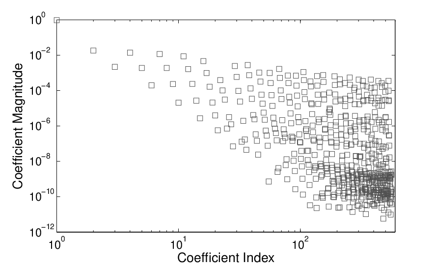
Our QoI is $\rho_{c}:=\rho(t=4,\Xi_{1},\Xi_{2})$, and we consider a Hermite PC expansion of total order $p=32$, giving $P=561$ basis functions to approximate $\rho_{c}$. This high-order approximation is necessary due to the large gradient of $\rho_{c}$ in terms of the random variables, as evidenced by the relatively slow decay of coefficients in the reference solution presented in Figure 5. This reference solution is computed using Gauss-Hermite quadrature approximation of the PC coefficients.

In Figure 6, we see plots of moments for the relative root-mean-squared error – between the reference and least squares solutions – as a function of the number of samples, $N$, obtained from 200 independent replications for each $N$. We find that the standard sampling fails to converge, while the asymptotic and coherence-optimal samplings lead to converged solution as $N$ is increased. We note that, in all cases, the standard sampling resulted in rank-deficient matrices $\bm{\Psi}$, and the reported results were generated using MATLAB’s lsqr function with a large number of iterations.

Following [34, 2, 35, 36], we next consider a $2$-D heat driven square cavity flow problem with uncertain wall temperature, as shown in Fig. 7. The left vertical wall has a deterministic, constant temperature $\tilde{T}_{h}$, referred to as the hot wall, while the right vertical wall has a stochastic temperature $\tilde{T}_{c}<\tilde{T}_{h}$ with constant mean $\bar{\tilde{T}}_{c}$, referred to as the cold wall. Both the top and bottom walls are assumed to be adiabatic. The reference temperature and the reference temperature difference are defined as $\tilde{T}_{ref}=(\tilde{T}_{h}+\bar{\tilde{T}}_{c})/2$ and $\Delta\tilde{T}_{ref}=\tilde{T}_{h}-\bar{\tilde{T}}_{c}$, respectively. Under the assumption of small temperature differences, i.e., Boussinesq approximation, the governing equations in dimensionless variables are given by

where $\bm{\hat{y}}$ is the unit vector $(0,1)$, $\bm{u}=(u,v)$ is velocity vector field, $T=(\tilde{T}-\tilde{T}_{ref})/\Delta\tilde{T}_{ref}$ is normalized temperature ($\tilde{T}$ denotes non-dimensional temperature), $p$ is pressure, and $t$ is time. Non-dimensional Prandtl and Rayleigh numbers are defined, respectively, as $\text{Pr}={\tilde{\mu}}\tilde{c}_{p}/\tilde{\kappa}$ and $\text{Ra}={\tilde{\rho}}{g}\beta\Delta\tilde{T}_{ref}{\tilde{L}}^{3}/({\tilde{\mu}}{\tilde{\kappa}})$, where the superscript tilde ($\tilde{~}$) denotes the non-dimensional quantities. Specifically, ${\tilde{\mu}}$ is molecular viscosity, ${\tilde{\kappa}}$ is thermal diffusivity, ${\tilde{\rho}}$ is density, ${g}$ is gravitational acceleration, the coefficient of thermal expansion is given by $\beta$, and ${\tilde{L}}$ is the reference length. In this example, the Prandtl and Rayleigh numbers are set to $\text{Pr}=0.71$ and $\text{Ra}=10^{6}$, respectively. For more details on the non-dimensional variables in (27), we refer the reader to [35, 34, 2]. On the cold wall, we use a (normalized) temperature distribution with stochastic fluctuations of the form

where $\bar{T}_{c}$ is a constant mean temperature. In (28), $\Xi_{i}$, $i=1,\dots,d$, are independent random variables uniformly distributed on $[-1,1]$. $\{\lambda_{i}\}_{i=1}^{d}$ and $\{\varphi_{i}(y)\}_{i=1}^{d}$ are the $d$ largest eigenvalues and the corresponding eigenfunctions of the exponential covariance kernel $C_{T_{c}T_{c}}(y_{1},y_{2})=\exp{\left(-\frac{|y_{1}-y_{2}|}{l_{c}}\right)}$, where $l_{c}$ is the correlation length. In this setting, a (semi-)analytic representation of the eigenpairs $(\lambda_{i},\varphi_{i}(y))$ in (28) is available, see, e.g., [37].

In our numerical tests, we let $(T_{h},\bar{T}_{c})=(0.5,-0.5)$, $d=20$, $l_{c}=1/21$, and $\sigma_{T}=11/100$. Our QoI, the vertical velocity component at $(x,y)=(0.25,0.25)$ denoted by $v(0.25,0.25)$, is expanded in the Legendre PC basis of total degree $p=4$ with only the first $P=2500$ basis functions retained. We seek to accurately reconstruct $v(0.25,0.25)$ with $N<P$ random samples of $\bm{\Xi}$ and the corresponding realizations of $v(0.25,0.25)$. These samples are constructed from a least squares reference solution constructed from these 2500 basis polynomials as computed from a large number of Monte Carlo samples.

References

- [1] R. Ghanem, P. Spanos, Stochastic Finite Elements: A Spectral Approach, Springer Verlag, 1991.
- [2] O. L. Maitre, O. Knio, Spectral Methods for Uncertainty Quantification with Applications to Computational Fluid Dynamics, Springer, 2010.
- [3] D. Xiu, Numerical Methods for Stochastic Computations: A Spectral Method Approach, Princeton University Press, 2010.
- [4] R. Smith, Uncertainty Quantification: Theory, Implementation, and Applications, Vol. 12, SIAM, 2013.
- [5] D. Xiu, G. Karniadakis, The Wiener-Askey polynomial chaos for stochastic differential equations, SIAM Journal on Scientific Computing 24 (2) (2002) 619–644.
- [6] C. Soize, R. Ghanem, Physical systems with random uncertainties: Chaos representations with arbitrary probability measure, SIAM Journal of Scientific Computing 26 (2) (2005) 395–410.
- [7] S. Hosder, R. Walters, R. Perez, A non-intrusive polynomial chaos method for uncertainty propagation in CFD simulations, in: th AIAA aerospace sciences meeting and exhibit, AIAA-2006-891, Reno (NV), 2006.
- [8] M. Berveiller, B. Sudret, M. Lemaire, Stochastic finite element: a non intrusive approach by regression, European Journal of Computational Mechanics/Revue Européenne de Mécanique Numérique 15 (1-3) (2006) 81–92.
- [9] A. Cohen, M. A. Davenport, D. Leviatan, On the stability and accuracy of least squares approximations., Foundations of Computational Mathematics 13 (5) (2013) 819–834.
- [10] G. Migliorati, F. Nobile, E. von Schwerin, R. Tempone, Approximation of quantities of interest in stochastic pdes by the random discrete projection on polynomial spaces, SIAM Journal on Scientific Computing 35 (3) (2013) A1440–A1460.
- [11] A. Chkifa, A. Cohen, G. Migliorati, F. Nobile, R. Tempone, Discrete least squares polynomial approximation with random evaluations; application to parametric and stochastic elliptic pdes, Also available as EPFL-MATHICSE report (2013) 35–2013.
- [12] B. Jones, A. Doostan, G. Born, Nonlinear propagation of orbit uncertainty using non-intrusive polynomial chaos, Journal of Guidance, Control, and Dynamics 36 (2) (2013) 430–444.
- [13] B. Jones, A. Doostan, Satellite collision probability estimation using polynomial chaos expansions, Advances in Space Research 52 (11) (2013) 1860–1875.
- [14] G. Migliorati, F. Nobile, E. Schwerin, R. Tempone, Analysis of discrete projection on polynomial spaces with random evaluations, Foundations of Computational Mathematics 14 (3) (2014) 419–456.
- [15] Z. Gao, T. Zhou, Choice of nodal sets for least square polynomial chaos method with application to uncertainty quantification, Commun. Comput. Phys (2014) 365–381.
- [16] T. Zhou, A. Narayan, Z. Xu, Multivariate discrete least-squares approximations with a new type of collocation grid, arXiv preprint arXiv:1401.0894.
- [17] T. Tang, T. Zhou, On discrete least square projection in unbounded domain with random evaluations and its application to parametric uncertainty quantification, arXiv preprint arXiv:1403.6579.
- [18] E. J. Candés, Y. Plan, A probabilistic and ripless theory of compressed sensing, Information Theory, IEEE Transactions on 57 (11) (2010) 7235–7254.
- [19] J. Hampton, A. Doostan, Compressive sampling of polynomial chaos expansions: convergence analysis and sampling strategies, Journal of Computational Physics In press, available online.
- [20] H. Rauhut, R. Ward, Sparse legendre expansions via l1-minimization, J. Approx. Theory 164 (5) (2012) 517–533.
- [21] G. Szegö, Orthongonal Polynomials, American Mathematical Society, American Mathematical Society, 1939.
- [22] D. Dominici, Asymptotic analysis of the hermite polynomials from their differential-difference equation, Journal of Difference Equations and Applications 13 (12) (2007) 1115–1128.
- [23] R. Askey, S. Wainger, Mean convergence of expansions in laguerre and hermite series, American Journal of Mathematics 87 (3) (1965) 695–708.
- [24] B. Muckenhoupt, Asymptotic forms for laguerre polynomials, Proceedings of the American Mathematical Society 24 (2) (1970) 288–292.
- [25] P. Nevai, T. Erdélyi, A. Magnus, Generalized jacobi weights, christoffel functions, and jacobi polynomials, SIAM Journal on Mathematical Analysis 25 (2) (1994) 602–614.
- [26] J. A. Tropp, User-friendly tail bounds for sums of random matrices, Foundations of Computational Mathematics 12 (4) (2012) 389–434.
- [27] A. Doostan, H. Owhadi, A non-adapted sparse approximation of PDEs with stochastic inputs, Journal of Computational Physics 230 (2011) 3015–3034.
- [28] L. Mathelin, K. Gallivan, A compressed sensing approach for partial differential equations with random input data, Commun. Comput. Phys. 12 (2012) 919–954.
- [29] L. Yan, L. Guo, D. Xiu, Stochastic collocation algorithms using -minimization, International Journal for Uncertainty Quantification 2 (3).
- [30] W. K. HASTINGS, Monte carlo sampling methods using markov chains and their applications, Biometrika 57 (1) (1970) 97–109.
- [31] W. R. Gilks, S. Richardson, D. J. Spiegelhalter, Markov chain Monte Carlo in practice, Vol. 2, CRC press, 1996.
- [32] A. Makeev, D. Maroudas, I. Kevrekidis, Coarse stability and bifurcation analysis using stochastic simulators: Kinetic Monte Carlo examples, The Journal of chemical physics 116 (23) (2002) 10083–10091.
- [33] O. L. Maître, H. Najm, R. Ghanem, O. Knio, Multi-resolution analysis of wiener-type uncertainty propogation schemes, J. Comput. Phys 197 (2004) 502–531.
- [34] O. LeMaitre, M. Reagan, H. Najm, R. Ghanem, O. Knio, A stochastic projection method for fluid flow. ii: Random process, J. Comp. Phys. 181 (2002) 9–44.
- [35] P. L. Quéré, Accurate solutions to the square thermally driven cavity at high rayleigh number, Computers & Fluids 20 (1) (1991) 29–41.
- [36] J. Peng, J. Hampton, A. Doostan, A weighted -minimization approach for sparse polynomial chaos expansions, Journal of Computational Physics 267 (2014) 92–111.
- [37] R. Ghanem, P. Spanos, Stochastic Finite Elements: A Spectral Approach, Dover, 2002.