On a molecular based Q-tensor model for liquid crystals with density variations

The molecular models for liquid crystals are based on microscopic statistical physics. By means of the cluster expansion, Onsager [2] pioneered the molecular field theory, in which the order parameter is the density function for the position and orientation of molecules. Onsager’s molecular model is established on sound physical principles, and contains no adjustable parameters. However, the molecular model is not clearly related to macroscopic properties, and the high dimension of the order parameter imposes considerable obstacles in computations. Based on Onsager’s molecular theory, the McMillan model [3] and a list of molecular models [4] [5] [6] parameterized the density function by some scalar order parameters to model the smectic phases. By lowering the dimensions, these model are very efficient in computations. However, the order parameters of these models are spatially invariant, so that they cannot model detailed physical phenomena with confined geometry and spatial variance.

On the other hand, a vector model for liquid crystals was phenomenologically proposed by Oseen [7], where the order parameter is a vector field ${\mathbf{n}}({\mathbf{x}})$ representing the director. As a development of Landau-Ginzburg theory and Oseen-Frank theory, Chen and Lubensky [8] introduced the density as another order parameter to characterize ${\mathbf{N}}$-${\mathbf{S_{A}}}$-${\mathbf{S_{C}}}$ phase transitions. The Chen-Lubensky model is famous for its conciseness. The internal coefficients can be measured through experiments. However, this model presumes liquid crystals to be uniaxial, and the director ${\mathbf{n}}$ is singular at defect points, which renders it difficult to characterize some small scale phenomena, such as defects and interfaces.

Overcoming the drawbacks of the molecular models and the vector models, the well-known Landau-de Gennes model [9] was proposed with the energy functional

where $A$, $B$, $C$, and $L_{i}$ are constants. The order parameter is a $3\times 3$ symmetric traceless tensor field $Q({\mathbf{x}})$, which is the second moment of molecules’ orientation at every point.

The Q-tensor is a desirable order parameter providing information on both the preferred molecular orientation and the degree of orientational order at every given point, while capturing essential physical properties. Various phenomena were studied with the Landau-de Gennes model, e.g. phase transitions in confined geometries [10] [11], wetting phenomena [12] [13], surface-induced bulk alignment [14] [15], and defects and disclinations [16] [17].

The order parameter and the energy functional of the Landau-de Gennes model are also simple enough to perform rigorous mathematical analysis. Ball and Majumdar proved that the energy of Landau-de Gennes model is unbounded from below as $L_{4}\neq 0$, and proposed to modify the entropy term from a polynomial into a thermotropic one in order to avoid the unboundedness [18]. Furthermore, Ball and Zarnescu proved that for simply-connected domains and in Sobolev space $W^{1,2}$ with corresponding boundary conditions, the Landau-de Gennes theory and the Oseen-Frank theory coincide [19].

Various generalizations of the Landau-de Gennes model [6] [20] [21] [22] were proposed to include smectic phases. The work of Pajak and Osipov [6] is a generalization of the McMillan model [3] and the Landau-de Gennes model, which starts from the self-consistent field theory and adopts the one mode approximation to parameterize the density function. The details of this model are provided in section 4.2. This model is efficient in computations, but the order parameters are spatially invariant, failing to characterize some physical phenomena with confined geometry and spatial variance. The works of Mukherjee [21] and Biscari et al. [22] are also generalizations of the Landau-de Gennes theory. The Q-tensor is coupled with the complex smectic order parameter, and the spatial inhomogeneity of the order parameters enables the model to characterize smectic phases. However, it is noteworthy that these models did not explain how the energy functionals were derived in details.

In a recent paper by Han et al. [1], a systematic way of modeling static liquid crystals with uniaxial molecules was proposed. To be more precise, starting from Onsager’s molecular theory, a new Q-tensor model was presented incorporating the Bingham closure and a Taylor expansion with truncation at low order moments. The coefficients in the new Q-tensor model were approximated in terms of the microscopic shape factor $\varepsilon=D/L$ by assuming the interaction potential to be the volume exclusion potential of rigid rod-like molecules. Here, $D$ is the diameter of the semisphere at the ends of the rods, and $L$ is the length of the rods. In modeling the nematic phase, the Oseen-Frank model and the Ericksen model were derived using the new Q-tensor model by assuming a constant density. Three elastic constants $K_{1}$, $K_{2}$, and $K_{3}$, measuring the strains on liquid crystals in deformation, were calculated analytically. In modeling the smectic phase, under the uniaxial assumption, some preliminary numerical results regarding ${\mathbf{I}}$-${\mathbf{N}}$-${\mathbf{S_{A}}}$ phase transitions were presented.

The energy functional of the new Q-tensor model in a modified version reads

where

Here, $\beta=\frac{1}{k_{B}T}$ is the thermodynamic beta. $c({\mathbf{x}})$ is the density. Q-tensor $Q({\mathbf{x}})$ is the traceless second moment of the orientational variable ${\mathbf{m}}$, and $Q_{4}({\mathbf{x}})$ is the traceless fourth moment of the orientational variable ${\mathbf{m}}$. $B_{Q}$ is the Bingham distribution parameters, and $1/Z({\mathbf{x}})$ is the normalizing constant for the Bingham distribution. The bulk energy $F_{bulk}$ contains the entropy and the quadratic terms of the order parameters. The second order elastic energy $F_{elastic,2}$ contains the derivative terms of the order parameters; the fourth order elastic energy $F_{elastic,4}$ contains the second order derivative terms of the order parameters. Note that here the fourth order elastic energy $F_{elastic,4}$ is truncated: only the positive definite terms are preserved in order to ensure the lower boundedness of the energy functional. The detailed descriptions of the energy functional are presented in the main body of this paper.

In this paper, regarding the new Q-tensor model as a phenomenological model, we focus on its density variation effects, and show its effectiveness in terms of mathematics, physics, and computations. The introduction of the density $c({\mathbf{x}})$ as another order parameter exhibits many benefits. It empowers the model to characterize the smectic phases, and to characterize the density variations in small scale phenomena such as defects and interfaces. Since a few Fourier modes are enough to characterize the profiles of the order parameters, the model can be solved with low computational costs. Numerical experiments are performed to study ${\mathbf{I}}$-${\mathbf{N}}$-${\mathbf{S_{A}}}$-${\mathbf{S_{C}}}$ phase transitions, and the results are compared with experimental results. The ${\mathbf{I}}$-${\mathbf{N}}$ interface problem is also studied in the new Q-tensor model setup, where the numerical results are compared with previous theoretical results and experimental results.

In addition, we will elaborate on the strong connections of the new Q-tensor model with the classical models of liquid crystals in three scales. Derived from Onsager’s molecular theory, the new Q-tensor model can generate all the other classical models with some assumptions and approximations. Figure 1 shows the classical models in three scales and their relations.

This paper is organized as follows. In section 2, we demonstrate the mathematical properties of the new Q-tensor model and the numerical methods to compute the energy functional. In section 3, the numerical results regarding ${\mathbf{I}}$-${\mathbf{N}}$-${\mathbf{S_{A}}}$-${\mathbf{S_{C}}}$ phase transitions and ${\mathbf{I}}$-${\mathbf{N}}$ interface are presented. In section 4, we compare the Q-tensor model with the classical models. We give several concluding remarks in section 5. Some detailed calculations involved in the paper are provided in the appendix.

In this paper, all vectors will be expressed by boldface letters. The juxtaposition of a pair of vectors ${\mathbf{m}}{\mathbf{n}}$ denotes the dyadic product of ${\mathbf{m}}$ and ${\mathbf{n}}$. Doubly contracted tensor products are represented by a colon. The Einstein summation convention for tensors is used.

The new Q-tensor model gives the free energy of liquid crystals as equation (2), with the definitions of notations as follows. Consider the rod-like liquid crystal molecules in domain $\Omega\subset{\mathbb{R}}^{3}$. The molecules take positional coordinate ${\mathbf{x}}\in\Omega$, and orientational coordinate ${\mathbf{m}}\in\mathbb{S}^{2}$. The positional coordinate ${\mathbf{x}}=\bar{\mathbf{x}}/L$ is dimensionless, which is the ratio of the physical position $\bar{\mathbf{x}}$ and the length of the molecules $L$. We introduce the density $c({\mathbf{x}})$ and the Q-tensor $Q({\mathbf{x}})$ as order parameters. The density $c({\mathbf{x}})$ is dimensionless, representing the number of molecules in volume $L^{3}$. The tensor $Q({\mathbf{x}})$ is the second moment of ${\mathbf{m}}$ with respect to $\rho$,

where $\rho$ is the probability density function of molecules with respect to orientation ${\mathbf{m}}$ at given position ${\mathbf{x}}$. This definition requires the Q-tensor to be a symmetric, traceless $3\times 3$ matrix whose eigenvalues $\{\lambda_{i}(Q)\}$ are constrained by the inequalities

Let $Q_{4}$ be the fourth moment of ${\mathbf{m}}$ in terms of $\rho$, which is defined as

where $(\cdot)_{sym}$ denotes the symmetrization of the tensor with respect to all permutations of indices.

Various closure models were proposed to represent the relationship between $Q_{4}$ and $Q$ [23]. Among various closure models, we choose the Bingham closure model, which has the following good properties.

• •

  The maximizer $\rho^{*}({\mathbf{x}},{\mathbf{m}})$, maximizing the entropy $\int_{\mathbb{S}^{2}}\rho\ln\rho\mathrm{d}{\mathbf{m}}$ subject to the Q-tensor $Q({\mathbf{x}})$ conforming (6) and (7), follows the Bingham distribution [18].

• •

  The Bingham closure automatically ensures (7), which preserve the physical meanings of the Q-tensor.

• •

  The dynamic Q-tensor model, derived from Doi’s kinetic theory using the Bingham closure, obeys the energy dissipation law [1].

• •

  Some numerical results show that the Bingham closure gives the best approximation to Doi’s kinetic theory in simulating complex flows of liquid-crystalline polymers [23]

The Bingham distribution of $\rho({\mathbf{x}},{\mathbf{m}})$ reads

where

and $B_{Q}({\mathbf{x}})$ is any traceless symmetric matrix in $\mathbb{R}^{3\times 3}$. Under this assumption, it has been proven that given any $Q({\mathbf{x}})$ which conforms (7), $B_{Q}({\mathbf{x}})$ and $\rho({\mathbf{x}},{\mathbf{m}})$ can be uniquely determined [24]. Therefore, the dimension of the probability density function $\rho({\mathbf{x}},{\mathbf{m}})$ reduces to five, the same as that of $Q({\mathbf{x}})$ and $B_{Q}({\mathbf{x}})$.

As a generalization of the Landau-de Gennes theory, the introduction of the density $c({\mathbf{x}})$ as another order parameter enables the model to characterize smectic phases and density variations in physical phenomena such as defects and interfaces. The major phases of rod-like molecule liquid crystals can be characterized by $c({\mathbf{x}})$ and $Q({\mathbf{x}})$ as

• •

  ${\mathbf{I}}$ phase: $c=\text{const}$, $Q=0$.

• •

  ${\mathbf{N}}$ phase: $c=\text{const}$, $Q=s({\mathbf{n}}{\mathbf{n}}-\frac{1}{3}\mathbf{I})=\text{const}$.

• •

  ${\mathbf{S_{A}}}$ phase: $c$ and $Q$ are one-dimensional and periodic. The director ${\mathbf{n}}$, defined as the principal eigenvector of Q-tensor, is parallel to the layer normal $\nabla c$.

• •

  ${\mathbf{S_{C}}}$ phase: $c$ and $Q$ are one-dimensional and periodic. The director ${\mathbf{n}}$ and the layer normal $\nabla c$ yield angle $\theta$, which represents the average of tilt angles between the rod-like molecules and the layer normal.

Biaxiality is an important property in smectic phases, and in other physical phenomena such as defects and interfaces. In this paper, biaxiality is given by a common mathematical definition

This definition requires the biaxiality $B({\mathbf{x}})$ within the interval $[0,1]$. If the Q-tensor is uniaxial, $B({\mathbf{x}})$ will be zero; if the Q-tensor shows strong biaxiality, $B({\mathbf{x}})$ will tend to one.

Other notations in the energy functional (2) are as follows. $\beta=\frac{1}{k_{B}T}$ is the thermodynamic beta. The $14$ dimensionless coefficients $A_{i}$, $G_{i}$, and $H_{i}$ are determined in terms of the microscopic molecule’s interaction potential, and are functions of temperature. We can infer their approximate range of values by assuming the interaction potential to be the volume exclusion potential of rigid rod-like molecules [1]. To ensure that the energy is bounded from below, it is necessary that $H_{1}$ and $H_{2}+\frac{2}{3}H_{3}+\frac{2}{3}H_{4}$ be positive. Otherwise, assuming the order parameters to be a series of highly oscillating functions, it is easy to show that the energy functional tends to negative infinity.

We consider the one-dimensional Q-tensor model. We note here that the one-dimensional case is significant and sufficiently representative, since ${\mathbf{I}}$, ${\mathbf{N}}$, ${\mathbf{S_{A}}}$, and ${\mathbf{S_{C}}}$ phases can all be represented in one dimension. For periodic boundary conditions, the spectral method is efficient and accurate enough to compute the energy functional, by representing the order parameters with a few Fourier modes. As another method, we can discretize the order parameters in nodal space and use finite difference method to calculate the derivatives.

Consider the reduced energy functional on the interval $[0,h]$, which takes the form

We consider how to numerically represent the order parameters. In the following, we will show that $Q(x)$ can be represented by five independent scalar variables $\lambda(x)$, $d(x)$, $\theta(x)$, $\beta(x)$, and $\gamma(x)$.

The Bingham assumption implies that $B_{Q}$, $Q$, and $Q_{4}$ are mutually determined and can be diagonalized simultaneously. Let the eigenvalue decomposition of $B_{Q}$ be $B_{Q,mn}=\hat{B}_{ij}T_{im}T_{jn}$, where $\hat{B}$ is a traceless diagonal matrix and $T$ is an orthogonal matrix. Using a change of variables in the integral (6) and (8), $Q$ and $Q_{4}$ can be represented as

Here, $\hat{Q}$ and $\hat{Q}_{4}$ are the diagonal forms of $Q$ and $Q_{4}$ respectively, which can be computed using $\hat{B}$ as

We use $\lambda$ and $d$ to represent the traceless diagonal matrix $\hat{B}$,

and use Euler angles $\theta$, $\beta$, and $\gamma$ to represent the orthogonal transformation matrix $T$,

Here, the first angle $\theta$ is the angle between the principal eigenvector of $Q$ and the x-axis.

Above all, the Q-tensor $Q(x)$ can be represented by $\lambda(x)$, $d(x)$, $\theta(x)$, $\beta(x)$, and $\gamma(x)$. In the meanwhile, $B_{Q}(x)$, $Z(x)$, and $Q_{4}(x)$ can also be computed using these five variables.

One way to discretize the order parameters is to expand them by Fourier modes

where $k=2\pi/h$. The dimension of variables is $12n+6$. The derivatives of $c\cdot Q$ and $c\cdot Q_{4}$ are calculated using Fast Fourier transform (FFT). In the following section, we use this method in computing the phase transition problem; empirically, $n=6$ is enough to characterize the profiles of the order parameters.

As another way to represent the order parameters, we can discretize the interval $[0,h]$ with $N$ nodes. The dimension of variables is $6N$. The derivatives of the order parameters are computed using the finite difference method. In the following section, we use this method in computing the ${\mathbf{I}}$-${\mathbf{N}}$ interface problem, and $N=50$ is accurate enough empirically.

The minimum of the energy functional can be found by standard methods. We use numerical differentiation to calculate the gradient of the objective function, and use quasi-Newton methods, such as the BFGS method to solve the optimization problem. The computations for both of the two problems discussed in the following section converge in about 100 steps with absolute precision of $1\times 10^{-5}$. The overall computational cost is as moderate as the cost of the Landau-de Gennes model.

It is worth pointing out that the Q-tensor model may have some local minima. In the simulation, we try different random initial values to ensure that we find the global minimum. In practice, there are no other local minimum points near the global minimum point.

First, we consider the phase transition problem. Since ${\mathbf{I}}$ and ${\mathbf{N}}$ phases are spatially homogeneous, and ${\mathbf{S_{A}}}$ and ${\mathbf{S_{C}}}$ phases are layered, we presume the solution to be periodic to reduce the computational costs. Therefore, we consider the domain $\Omega=[0,h]$, and assume that the order parameters enjoy the periodic boundary conditions. Given the average density $c_{0}$, we need to minimize the average free energy $F_{h}/h$, where $F_{h}$ is defined as equation (12).

We have the optimization problem

Spectral methods are used to calculate the free energy. The period $h$, which is also a variable that needs to be optimized, represents the layer thickness in the smectic phases. Figure 2 illustrates the microscopic configuration of molecules of the smectic phases. The following phase transitions are found given various sets of $G_{4}$ and $H_{3}$.

• •

  $G_{4}=G_{4}^{(0)}\times 3.9$, $H_{3}=H_{3}^{(0)}\times 1.7$.

  ${\mathbf{I}}{\mathrel{\to}^{c\approx 45.2}}{\mathbf{N}}{\mathrel{\to}^{c\approx 46.5}}{\mathbf{S_{A}}}{\mathrel{\to}^{c\approx 50.3}}{\mathbf{S_{C}}}$.

• •

  $G_{4}=G_{4}^{(0)}$, $H_{3}=H_{3}^{(0)}$.

  ${\mathbf{I}}{\mathrel{\to}^{c\approx 45.2}}{\mathbf{N}}{\mathrel{\to}^{c\approx 50.6}}{\mathbf{S_{A}}}$.

• •

  $G_{4}=G_{4}^{(0)}\times 2$, $H_{3}=H_{3}^{(0)}\times 6$.

  ${\mathbf{I}}{\mathrel{\to}^{c\approx 45.2}}{\mathbf{N}}{\mathrel{\to}^{c\approx 50.6}}{\mathbf{S_{C}}}$.

The one-dimensional phase diagrams of ${\mathbf{I}}$-${\mathbf{N}}$-${\mathbf{S_{A}}}$-${\mathbf{S_{C}}}$ transitions are presented using $F_{min}-c_{0}$ coordinates in Figure 4, and using $\theta-c_{0}$ coordinates in Figure 4.

As the average density $c_{0}$ increases, the system exhibits ${\mathbf{I}}$, ${\mathbf{N}}$, ${\mathbf{S_{A}}}$, and ${\mathbf{S_{C}}}$ phases sequentially. As shown in Figure 4, ${\mathbf{I}}$-${\mathbf{N}}$ and ${\mathbf{N}}$-${\mathbf{S_{A}}}$ phase transitions are first order. ${\mathbf{I}}$ and ${\mathbf{N}}$ phases coexist as $c_{0}$ is within $45.2\pm 0.2$; ${\mathbf{N}}$ and ${\mathbf{S_{A}}}$ phases coexist as $c_{0}$ is within $46.5\pm 0.2$. The free energies of both phases in these regions are local minima, which are confirmed by numerically evaluating the Hessian matrix at the minimum points. It is noteworthy that the ${\mathbf{N}}$-${\mathbf{S_{A}}}$ phase transition is of weak first order: at both of the local minimum points, the smallest eigenvalue of the Hessian is near 0, which indicates that the energy barrier between these two stable phases is rather small. From the physical point of view, the average density $c_{0}=45.2$ states that on average there are $45.2$ liquid crystal molecules with shape factor $\varepsilon=0.1$ in a cube with volume $L^{3}$, and the molecules take up roughly $35$ percent the volume of the entire space.

As shown in Figure 4, the ${\mathbf{S_{A}}}$-${\mathbf{S_{C}}}$ phase transition is of second order. After $c_{0}$ exceeds $50.3$, the tilt angle of director increases from $0$ to $5$ degrees continuously. In one layer, the centers of molecules align in order, but not exactly in a plane, which renders the layer thickness larger than the length of molecules. The optimized layer thickness for both ${\mathbf{S_{A}}}$ and ${\mathbf{S_{C}}}$ phases is roughly $1.81L$, i.e. $1.81$ times the length of the molecule, and it varies slightly within the order $0.005L$ as the average density increases. The layer thickness is quite sensitive to the coefficients $G_{i}$ and $H_{i}$. If $H_{3}$ decreases from $H_{3}^{(0)}\times 3.9$ to $H_{3}^{(0)}\times 3.6$, the layer thickness will decrease from $1.81L$ to $1.74L$. This relation between the coefficients and the layer thickness is explained using the vector model, with its details discussed in Section 4.3.

Figure 5 shows the components of the free energy as the average density increases, which exhibits the order of transitions more clearly. The definitions of these components are given as (3), (4), and (5), and the entropy is the first part of the bulk energy $F_{bulk}$. The entropy decreases at the beginning. It has positive leaps at ${\mathbf{I}}$-${\mathbf{N}}$ and ${\mathbf{N}}$-${\mathbf{S_{A}}}$ critical points, and finally increases gradually. The bulk energy increases gradually with a leap at ${\mathbf{N}}$-${\mathbf{S_{A}}}$ critical point. The elastic energy $F_{elastic,2}$ and $F_{elatic,4}$ are zero in ${\mathbf{I}}$ and ${\mathbf{N}}$ phases. The second order elastic energy $F_{elastic,2}$ drops and continuously decreases after reaching ${\mathbf{N}}$-${\mathbf{S_{A}}}$ critical point, while the fourth order elastic energy $F_{elastic,4}$ soars up and continuously increases after ${\mathbf{N}}$-${\mathbf{S_{A}}}$ point, with a smaller magnitude than $F_{elastic,2}$. All these components at ${\mathbf{S_{A}}}$-${\mathbf{S_{C}}}$ critical point are continuous. The total energy increases steadily without significant leaps.

The second order elastic energy $F_{elastic,2}$ contains two parts: derivative terms in the density $c(x)$ and the Oseen-Frank energy which contains the derivative terms of director ${\mathbf{n}}$. This decomposition is further discussed in Section 4.3. In smectic phases, the Oseen-Frank energy is zero for there is no distortion of the director. The derivative terms in the density $c(x)$ in $F_{elastic,2}$ with negative coefficients are the reason for the density-varied phases to have a lower free energy. The second order derivative terms in the density in $F_{elastic,4}$ with positive coefficients are the reason for the total energy to be stable.

The representative use of the order parameters and the biaxiality characterizing the smectic phase is shown in Figure 6. The relative density $c_{r}(x)$ is defined as $c_{r}(x)=c(x)/c_{0}$. The Q-tensor can be written as $Q=s(\mathbf{nn}-\frac{1}{3}\mathbf{I})+b(\mathbf{n^{\prime}n^{\prime}}-\frac{1}{3}\mathbf{I})$, where $\mathbf{n^{\prime}}$ is perpendicular to the director ${\mathbf{n}}$; $s(x)$ is the principal nematic order parameter, and $b(x)$ characterizes biaxial effects. The biaxiality $B(x)$ is defined as equation (11). In the smectic phase, the relative density $c_{r}(x)$ and order parameter $s(x)$ fluctuate within one layer. The maximum point of $c(x)$ and $s(x)$ are identical, where the centers of molecules concentrate and the molecules are more likely to point to the preferred direction. In the ${\mathbf{S_{A}}}$ phase, the biaxiality $B(x)$ vanishes, which supports that the uniaxial approximation often adopted in modeling ${\mathbf{S_{A}}}$. In ${\mathbf{S_{C}}}$ phase, $B(x)$ vanishes when the relative density $c_{r}(x)$ is large. At the region between two layers where the relative density $c_{r}(x)$ is small, the biaxiality $B(x)$ is large. This phenomena can be explained intuitively: the group of molecules at the vicinity region between two layers have more freedom of orientation and are less symmetric than the group of molecules at the center of one layer.

The ${\mathbf{I}}$-${\mathbf{N}}$-${\mathbf{S_{A}}}$ transitions and ${\mathbf{I}}$-${\mathbf{N}}$-${\mathbf{S_{C}}}$ transitions are presented given other sets of coefficients. The one-dimensional phase diagrams are presented using $F_{min}-c_{0}$ coordinates in Figure 8 characterizing ${\mathbf{I}}$-${\mathbf{N}}$-${\mathbf{S_{A}}}$ transitions, and in Figure 8 characterizing ${\mathbf{I}}$-${\mathbf{N}}$-${\mathbf{S_{C}}}$ transitions. In the ${\mathbf{S_{A}}}$ phase, the layer thickness is roughly $1.52L$. In ${\mathbf{S_{C}}}$ phase, the layer thickness is roughly $1.92L$, and the tilt angle is $23$ degree. The ${\mathbf{N}}$-${\mathbf{S_{C}}}$ transition is also first order.

According to liquid crystal experiments, the ${\mathbf{I}}$-${\mathbf{N}}$ transition and the ${\mathbf{N}}$-${\mathbf{S_{A}}}$ transition could be either first or second order, depending on the liquid crystal materials. The ${\mathbf{I}}$-${\mathbf{N}}$ transition is most commonly believed to be of first order [26], but some experiments of MBBA [(4-Butyl-phenyl)-(4-methoxy-benzylidene)-amine] reported a second order transitions [27]. The study of 8CB-10CB mixtures [28] confirmed the prediction made by Halperin et al. that fluctuation change the second order ${\mathbf{N}}$-${\mathbf{S_{A}}}$ transition into a weak first order one. The study of 4-n-alkoxybenzylidene-4’-phenylazoaniline [29] drew the conclusion that decreasing the length of the alkyl end chain drives the first order ${\mathbf{N}}$-${\mathbf{S_{A}}}$ transition to be second order. According to Monte-Carlo simulation based on molecular theory, assuming the molecule’s shape to be spherocylindrical, McGrother et al. [30], Bolhuis et al. [31], and Lolson et al. [32] showed that the ${\mathbf{N}}$-${\mathbf{S_{A}}}$ transition is a first order one, but it tends to become continuous as the shape factor $L/D\rightarrow\infty$. In comparison, our simulation results predict the ${\mathbf{I}}$-${\mathbf{N}}$ transition is of first order; the energy barrier between the ${\mathbf{N}}$ and ${\mathbf{S_{A}}}$ phases is rather small, which indicates that the ${\mathbf{N}}$-${\mathbf{S_{A}}}$ transition is of weak first order.

For the ${\mathbf{S_{A}}}$-${\mathbf{S_{C}}}$ transition, the study of 8S5 [4-n-pentyl-phenylthiol-4’-n-octyloxybenzoate] [33] reported a second order transition, and the tilt angle increases from $0$ degree to $20$ degree continuously. The study of C7 [4-(3-methyl-2-chloropentanoyloxy)-4’-heptyloxybiphenyl] [34] reported a first order ${\mathbf{S_{A}}}$-${\mathbf{S_{C}}}$ transition, and the tilt angle ranges from 0 to 34 degree. In our simulations, the ${\mathbf{S_{A}}}$-${\mathbf{S_{C}}}$ transition is of second order, and the tilt angle ranges from 0 to 23 degree. For the smectic layer thickness, most experiments indicated that the layer thickness of the smectic phase is around the molecule’s length $L$. A study of 8CB [4’-n-octyl-4-cyanobiphenyl] and 8OCB [4’-n-octyloxy-4-cyanobiphenyl] [35] showed that when molecules form dimers, one smectic layer would contain two molecule layer overlapped a bit, such that the layer thickness of the smectic phase is larger than $L$ but within $2L$. In our simulations, the predicted layer thickness is larger than most experiments results. However, our predicted layer thickness is in a reasonable range, which is larger than the length $L$ of the molecules but within $2L$ varying with different coefficients.

Consider the liquid crystals in the entire space. ${\mathbf{I}}$ and ${\mathbf{N}}$ are at two opposite ends of the space, sharing the same chemical potential and the same grand potential density. Assume the problem is one dimensional, and the order parameters vary in one dimension and are homogeneous in the other two dimensions. Given the angle $\theta$ between the interface normal and the director of the nematic phase, the configuration of the interface is determined. The microscopic configuration of molecules of ${\mathbf{I}}$-${\mathbf{N}}$ interface is illustrated as Figure 9.

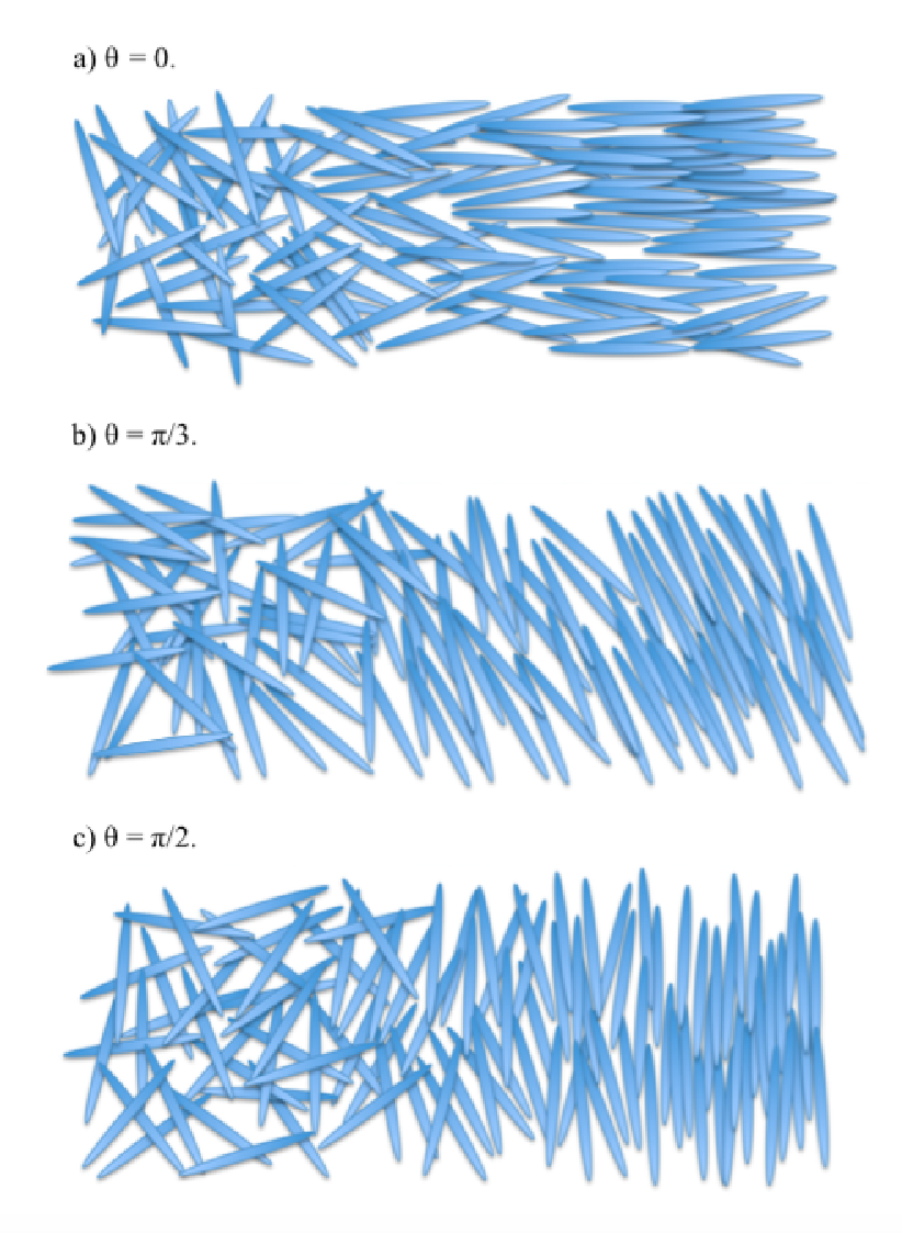
Consider the region $\Omega=[-h,h]$. We need to minimize the grand potential

under proper boundary conditions. The chemical potential is chosen to meet the coexistence condition, $\mu=3.407$. The order parameters for the stable isotropic phase are $c=43.57$ and $Q=0$; the order parameters for the stable nematic phase are $c=48.30$ and $Q=s({\mathbf{n}}{\mathbf{n}}-\frac{1}{3}{\mathbf{I}})$ with $s=0.667$. We anchor the angle $\theta$ between the director and the interface normal to be constant all over the space, and perform simulations with a series of $\theta$. Thus, the boundary conditions are

where $\theta_{0}=0$, $\pi/8$, $\pi/4$, $3\pi/8$, $\pi/2$. The length $h$ is chosen large enough, which is $7L$ in our computations. The coefficients $A_{i}$, $G_{i}$, and $H_{i}$ are given in equations (18) with $G_{4}=G_{4}^{(0)}=0.02374$, $H_{3}=H_{3}^{(0)}=0.00063$. Note that the coefficients $G_{i}$ here are all deduced by assuming the interaction potential to be the volume exclusion potential of rigid rod-like molecules. The results are summarized as follows.

Figure 10 (a) shows the profile of the density $c(x)$. The density profile for tilt angle $\theta$ greater than $\frac{\pi}{4}$ is a monotonically increasing function; nevertheless, for the tilt angle smaller than $\frac{\pi}{4}$, it displays a shallow dip near the isotropic side of the interface, and a small oscillation near the nematic side of the interface. The shallow dip near the isotropic side was captured by Chen and Noolandi [36] in numerical simulation of Onsager’s molecular theory, in which it was explained by the competition between the entropy and the excluded-volume interaction. The oscillating behavior was noticed by Allen [38] in Monte Carlo simulations; however, in Monte Carlo simulations, the oscillating behavior emerged for all cases of the tilt angle, and was explained as boundary effects. In the new Q-tensor model, the oscillating behavior can be explained by the negative coefficients of the derivative terms of density $c(x)$: with oscillation, the elastic energy $F_{elastic,2}$ can be lower. On the contrary, the fourth order elastic energy $F_{elastic,4}$ serves to stabilize the energy at the interface. The interfacial width of the density is roughly $3L$. It is at its narrowest at $\theta=\frac{\pi}{2}$.

Figure 10 (b) shows the principal nematic order parameter $s(x)$. Unlike the density profile, the profile of $s(x)$ is always a monotonic function. The centers of the profiles for $c(x)$ and $s(x)$ are different. There is a ”phase shift” for $s(x)$ to the isotropic side with roughly $0.5L$ compared to the density profile. Unlike the density profile, the interfacial width of $s(x)$ remains identical at $3L$ as tilt angle $\theta$ increases.

The interfacial width is not sensitive to the coefficients $H_{i}$. No matter how we alter the coefficients $H_{i}$ with an order of magnitude, the interfacial width is always roughly $3L$; nevertheless, as $H_{i}$ increases, the oscillation near the nematic side is mitigated but still exists.

Figure 10 (c) shows the biaxiality parameter $b(x)$. The biaxial effect only appears significantly in the interfacial region. It is opposite between the isotropic side and the nematic side, and is stronger at the isotropic side. The biaxiality is the strongest for $\theta=\frac{\pi}{2}$. There is no biaxiality for the $\theta=0$ case because of the rotational symmetry. In general, the biaxial effect for ${\mathbf{I}}$-${\mathbf{N}}$ interface is quite weak.

Figure 11 shows the dependence of the isotropic-nematic surface energy on the angle $\theta$. The surface energy is defined as the difference between the grand potential of the interface and that of the isotropic phase. The surface energy is a monotonic function of the tilt angle and has a minimum at $\theta=\frac{\pi}{2}$ with value $\sigma=0.100k_{B}T/(LD)$. Therefore, the interface prefers to have a tilt angle of $\frac{\pi}{2}$, which is the configuration as Figure 9 (c). In another word, if we do not assume the tilt angle $\theta$ constant, but just anchor it at the boundary, it would tend to $\frac{\pi}{2}$ at the interface, which was the setup and situation in the study by Monte Carlo simulations [38].

There are several previous studies of the ${\mathbf{I}}$-${\mathbf{N}}$ interface problem investigated using Onsager’s molecular theory with volume exclusion potential for rod-like molecules [36] [37] [38]. These simulations gave the interfacial width roughly at $2L$, which agree with the new Q-tensor model. Chen and Noolandi [36] predicted that the surface energy attains minimum at $\pi/2$ with value $\sigma=0.183k_{B}T/(LD)$. Koch and Harlen [37] used a generalization of Onsager’s approach and did a more comprehensive investigation. They predicted that the surface energy attains minimum at $\pi/2$ with value $\sigma=0.316k_{B}T/(LD)$. Our new Q-tensor model gives it a lower value $\sigma=0.100k_{B}T/(LD)$. Since the new Q-tensor model is a phenomenological model, and we alter the coefficients in our models, the value of the surface energy is only comparable in orders. To find an accurate value of the surface energy, it is better to use Onsager’s molecular theory.

The experimental study of MBBA [39] showed that the surface energy attains minimum at the tilt angle $\pi/2$, which is consistent with our calculations. However, the study of nCB [40] showed that the minimum of surface energy is attained at a tilt angle close to $\pi/3$. In the meanwhile, the experimental values of the interfacial width for the nCB are of the order of $400-700\mathring{A}$ (with molecule’s length about $20-30\mathring{A}$), in which the ratio is much larger than the ratio in our work and numerical simulations with hard rod molecules [36] [37] [38]. The numerical simulation of the ${\mathbf{I}}$-${\mathbf{N}}$ interface problem in modeling specific materials is still under investigation.

De Gennes pioneered the Q-tensor, which provides information on both the preferred molecular orientation and the degree of orientational order, to describe nematics phases [9]. Later on, by exploiting an analogy between smectic liquid crystals and superconductors, de Gennes again proposed an independent, complex order parameter that allows for the description of nematic-smectic phase transitions [41]. Successive models generalized the Landau-de Gennes model and coupled the nematic order tensor with the complex smectic order parameter. In the work of Biscari et al. [22], the free energy contained the polynomial terms and the first order derivative terms. In the work of Mukherjee [21], the free energy contained the polynomial terms, the first order and the second order derivative terms of these order parameters. These models successfully modeled the ${\mathbf{I}}$, ${\mathbf{N}}$, ${\mathbf{S_{A}}}$, and ${\mathbf{S_{C}}}$ phases with computational efficiency. However, it is noteworthy that the complex order parameter is not suitable for numerical simulations of liquid crystals in confined geometries, such as disclinations and defects. The work of Pevnyi et. al. [42] addressed the above problem and replaced the complex order parameter with the density $c({\mathbf{x}})$. The other order parameter ${\mathbf{n}}$ entered the free energy through the second order tensor $n_{i}n_{j}$, so we regard this model as a tensor model. This model gave reasonable numerical results to model the ${\mathbf{S_{A}}}$ phase in confined geometries with defects. The free energy contains the polynomial terms of the density, and the second order derivative terms of the order parameters, which can be viewed as a reduced case of the new Q tensor model.

The new Q-tensor model are more generalized comparing to the above models. For the new Q-tensor model, the entropy term is in the thermotropic form defined by Ball and Majumdar [18], but no longer has the polynomial terms as in the Landau-de Gennes model. Such an entropy term ensures the boundedness of the eigenvalues of the Q-tensor, preserving its physical meaning. If we assume $c({\mathbf{x}})$ is constant, $F_{bulk}+F_{elastic,2}$ would degenerate to the energy functional of the Landau-de Gennes model, which is able to characterize the stable nematic phase [18].

References

- [1] J. Han, Y. Luo, W. Wang, P. Zhang, and Z. Zhang, From microscopic theory to macroscopic theory: a systematic study on modeling for liquid crystals, Archive for Rational Mechanics and Analysis, 215.3 (2014), pp. 741-809.
- [2] L. Onsager, The effects of shape on the interaction of colloidal particles, Annals of the New York Academy of Sciences, 51 (1949), pp. 627-659.
- [3] W. L. McMillan, Simple molecular model for the smectic-A phase of liquid crystals, Physical Review A, 4 (1971), 1238.
- [4] L. Mederos, and D. E. Sullivan, Molecular theory of smectic-A liquid crystals, Physical Review A, 39 (1989), 854.
- [5] M. V. Gorkunov, M. A. Osipov, N. Kapernaum, D. Nonnenmacher, and F. Giesselmann, Molecular theory of smectic ordering in liquid crystals with nanoscale segregation of different molecular fragments, Physical Review E, 84 (2011), 051704.
- [6] G. Pajak, and M. A. Osipov, Unified molecular field theory of nematic, smectic-A, and smectic-C phases, Physical Review E, 88 (2013), 012507.
- [7] C. W. Oseen, The theory of liquid crystals, Transactions of the Faraday Society, 29 (1933), pp. 883-899.
- [8] J. Chen, and T. C. Lubensky, Landau-Ginzburg mean-field theory for the nematic to smectic-C and nematic to smectic-A phase transitions, Physical Review A, 14 (1976), 1202.
- [9] P. G. de Gennes, Short range order effects in the isotropic phase of nematics and cholesterics, Molecular Crystals and Liquid Crystals, 12 (1971), pp. 193-214.
- [10] P. Sheng, Boundary-layer phase transition in nematic liquid crystals, Physical Review A, 26 (1982), 1610.
- [11] S. Kralj, S. Žumer, and D. W. Allender, Nematic-isotropic phase transition in a liquid-crystal droplet, Physical Review A, 43 (1991), 2943.
- [12] T. J. Sluckin, and A. Poniewierski, Novel surface phase transition in nematic liquid crystals: Wetting and the Kosterlitz-Thouless transition, Physical review letters, 55 (1985), 2907.
- [13] M. Nobili, and G. Durand, Disorientation-induced disordering at a nematic-liquid-crystal–solid interface, Physical Review A, 46 (1992), R6174.
- [14] D. Johannsmann, H. Zhou, P. Sonderkaer, H. Wierenga, B. O. Myrvold, and Y. R. Shen, Correlation between surface and bulk orientations of liquid crystals on rubbed polymer surfaces: Odd-even effects of polymer spacer units, Physical Review E, 48 (1993), 1889.
- [15] X. Zhuang, L. Marrucci, and Y. R. Shen, Surface-monolayer-induced bulk alignment of liquid crystals, Physical review letters, 73 (1994), pp. 1513-1516.
- [16] N. Schopohl, and T. J. Sluckin, Defect core structure in nematic liquid crystals, Physical review letters, 59 (1987), 2582.
- [17] J. Fukuda, M. Yoneya, and H. Yokoyama, Defect structure of a nematic liquid crystal around a spherical particle: Adaptive mesh refinement approach, Physical Review E, 65 (2002), 041709.
- [18] J. M. Ball, and A. Majumdar, Nematic liquid crystals: from Maier-Saupe to a continuum theory, Molecular Crystals and Liquid Crystals, 525 (2010), pp. 1-11.
- [19] J. M. Ball, and A. Zarnescu, Orientable and non-orientable line field models for uniaxial nematic liquid crystals, Molecular crystals and liquid crystals, 495 (2008), pp. 221-573.
- [20] M. Vissenberg, S. Stallinga, and G. Vertogen, Generalized Landau-de Gennes theory of uniaxial and biaxial nematic liquid crystals, Physical Review E, 55 (1997), 4367.
- [21] P. K. Mukherjee, Nematic-smectic-A-smectic-C multicritical point: An alternative model, The European Physical Journal E, 33 (2010), pp. 175-181.
- [22] P. Biscari, M. C. Calderer, and E. M. Terentjev, Landau–de Gennes theory of isotropic-nematic-smectic liquid crystal transitions, Physical Review E, 75 (2007), 051707.
- [23] J. Feng, C. V. Chaubal, and L. G. Leal, Closure approximations for the Doi theory: Which to use in simulating complex flows of liquid-crystalline polymers?, Journal of Rheology (1978-present), 42 (1998), pp. 1095-1119.
- [24] S. Li, W. Wang, and P. Zhang, Local well-posedness and Erickson-Leslie limit of a molecule-based Q-tensor model, arXiv:1410.3286 [math.AP].
- [25] J. Xu, and P. Zhang, From microscopic theory to macroscopic theory - symmetries and order parameters of rigid molecules, Science China Mathematics, 57 (2014), pp. 443-468.
- [26] P. G. de Gennes, and J. Prost, The physics of liquid crystals, Oxford University Press, USA, (1995).
- [27] T. W. Stinson III, and J. D. Litster, Pretransitional phenomena in the isotropic phase of a nematic liquid crystal, Physical Review Letters, 25 (1970), 503.
- [28] M. A. Anisimov, P. E. Cladis, E. E. Gorodetskii, D. A. Huse, V. E. Podneks, V. G. Taratuta, W. Saarloos, and V. P. Voronov, Experimental test of a fluctuation-induced first-order phase transition: The nematic – smectic-A transition, Physical Review A, 41 (1990), 6749.
- [29] J. W. Doane, R. S. Parker, B. Cvikl, D. L. Johnson, and D. L. Fishel, Possible Second-Order Nematic – smectic-A Phase Transition, Physical Review Letters, 28 (1972), 1694.
- [30] S. C. McGrother, D. C. Williamson, and G. Jackson, A re‐examination of the phase diagram of hard spherocylinders, The Journal of chemical physics, 104 (1996), 6755.
- [31] P. Bolhuis, and D. Frenkel, Tracing the phase boundaries of hard spherocylinders, Journal of chemical physics, 106 (1997), pp. 666-687.
- [32] J. M. Polson, and D. Frenkel, First-order nematic-smectic phase transition for hard spherocylinders in the limit of infinite aspect ratio, Physical Review E, 56 (1997), R6260.
- [33] C. R. Safinya, M. Kaplan, J. Als-Nielsen, R. J. Birgeneau, D. Davidov, J. D. Litster, D. L. Johnson, and M. E. Neubert, High-resolution x-ray study of a smectic-A – smectic-C phase transition, Physical Review B, 21 (1980), 4149.
- [34] C. Bahr, and D. Fliegner, Behavior of a first-order smectic-A–smectic-C transition in free-standing liquid-crystal films, Physical Review A, 46 (1992), 7657.
- [35] J. E. Lydon, and C. J. Coakley, A structural study of the smectic mesophases of two biphenyl compounds and an x-ray investigation of the miscibility criterion, Le Journal de Physique Colloques, 36 (1975), C1-45.
- [36] Z. Y. Chen, and J. Noolandi, Numerical solution of the Onsager problem for an isotropic-nematic interface, Physical Review A, 45 (1992), 2389.
- [37] D. L. Koch, and O. G. Harlen, Interfacial tension at the boundary between nematic and isotropic phases of a hard rod solution, Macromolecules, 32 (1999), pp. 219-226.
- [38] M. P. Allen, Molecular simulation and theory of the isotropic–nematic interface, The Journal of Chemical Physics, 112 (2000), pp. 5447-5453.
- [39] D. Langevin, and M. A. Bouchiat, Molecular order and surface tension for the nematic-isotropic interface of MBBA, deduced from light reflectivity and light scattering measurements, Molecular Crystals and Liquid Crystals, 22 (1973), pp. 317-331.
- [40] S. Faetti, and V. Palleschi, Nematic-isotropic interface of some members of the homologous series of 4-cyano-4’-(n-alkyl) biphenyl liquid crystals, Physical Review A, 30 (1984), 3241.
- [41] P. G. de Gennes, An analogy between superconductors and smectics A, Solid State Communications, 10 (1972), pp. 753-756.
- [42] M. Y. Pevnyi, J. V. Selinger, and T. J. Sluckin, Modeling smectic layers in confined geometries: Order parameter and defects, Physical Review E, 90 (2014), 032507.
- [43] W. Maier, and A. Saupe, Eine einfache molekularstatistische Theorie der nematischen kristallinflussigen Phase. Teil I, Zeitschrift Naturforschung Teil A, 14 (1959), 882.