Improvements to stellar structure models, based on a grid of 3D convection simulations. II. Calibrating the mixing-length formulation
Abstract
We perform a calibration of the mixing length of convection in stellar structure models against realistic 3D radiation-coupled hydrodynamics (RHD) simulations of convection in stellar surface layers, determining the adiabat deep in convective stellar envelopes.
The mixing-length parameter is calibrated by matching averages of the 3D simulations to 1D stellar envelope models, ensuring identical atomic physics in the two cases. This is done for a previously published grid of solar-metallicity convection simulations, covering from 4 200 K to 6 900 K on the main sequence, and 4 300–5 000 K for giants with .
Our calibration results in an varying from 1.6 for the warmest dwarf, which is just cool enough to admit a convective envelope, and up to 2.05 for the coolest dwarfs in our grid. In between these is a triangular plateau of . The Sun is located on this plateau and has seen little change during its evolution so far. When stars ascend the giant branch, they largely do so along tracks of constant , with decreasing with increasing mass.
Keywords:
Stars: atmospheres – stars: evolution – convection1 Introduction
Due to the lack of a better theory of convection in stars, the mixing-length theory (Böhm-Vitense, 1958, MLT) has been in use for more than half a century. By far the largest part of the solar convection zone is very close to adiabatic, and the stratification in the bulk of the convection zone is therefore determined by the adiabatic gradient, , of temperature, , and pressure, . Convection is so efficient that the actual gradient, , need only be slightly larger than the adiabatic one, to transport the entire energy flux. In most of the convection zone the super-adiabatic gradient, , is small enough, , to have no effect on the structure of the star. We therefore have no need for a theory of convection here, except as a means to determine the adiabat of the convection zone.
This picture changes dramatically near the boundaries, especially near the upper boundary of a convective envelope. Here convection becomes exceedingly inefficient in transporting the energy flux, as radiative energy transport takes over. For the Sun, this layer of appreciable superadiabaticity only occurs in the outermost 1 Mm, just below the photosphere—the region where the gas becomes optically transparent and radiation escapes. This layer, however thin, is crucial for the star as a whole, as it is the star’s insulation against the cold of space. In other words, this layer constitutes the outer boundary condition for stellar models. It is the interaction between convection and radiative transfer in this layer that sets up the entropy jump at the top of the convection zone, and hence determines the adiabat of the convection zone. Modelling stellar atmospheres is complicated and computationally expensive and beyond the scope of normal stellar structure calculations. Instead, the structure modeller adopts results from atmosphere models that describe the radiative transfer through the atmosphere, and, in particular, the photospheric transition from optically thick to optically thin. One solution that we also adopt is to describe this transition by the behaviour of temperature, , with optical depth, , known as a relation (Henyey, Vardya & Bodenheimer, 1965, e.g.). With the radiative components fixed, the adiabat is then determined by the parameters of the MLT formulation.
Hotter, late A-type stars, close to the line in the HR diagram where stars loose their convective envelopes, have such shallow convective envelopes that they do not reach an adiabat. There, convection is inefficient and transports only a minor fraction of the flux, while the temperature fluctuations and the turbulent pressure are appreciable even at the bottom of the convection zone. This is the prediction of any realistic formulation of convection, and is confirmed by convection simulations (Freytag, Ludwig & Steffen, 1996; Kupka, Ballot & Muthsam, 2009; Freytag & Steffen, 2005; Trampedach, 2005). At the other end of the spectrum we find the cool M dwarfs that are fully convective. Giants, on the other hand, are dominated by extensive convective envelopes, and strongly condensed cores. This spans the range of stars for which the present work applies.
With the advances in atomic physics as applied to astrophysics, i.e., the equation of state (Hummer & Mihalas, 1988; Saumon, Chabrier & Horn, 1995; Nayfonov et al., 1999; Gong, Däppen & Zejda, 2001; Rogers & Nayfonov, 2002; Militzer & Hubbard, 2013, EOS, e.g.,) and opacities (Kurucz, 1992b; Rogers & Iglesias, 1992; Alexander & Ferguson, 1994; Seaton, 1995; Iglesias & Rogers, 1996; Badnell et al., 2005; Ferguson et al., 2007), by far the most uncertain aspects of stellar models are associated with dynamical phenomena: semi-convection, rotational mixing, mixing by g modes, convective overshooting and the most prominent: convection itself. Phenomena that all involve turbulence, non-locality and non-linearity, which make them less amenable to analytical formulations.
The present paper is part of an effort to improve on stellar structure models, by using results from a grid of realistic 3D hydrodynamical simulations of stellar surface convection in late-type stars. This grid of simulations is presented in more detail by Trampedach et al. (2013). The first paper in this series deals with the radiative part of the stellar surface problem and presents relations derived from the simulations (Trampedach et al., 2014, Paper I). The present paper is Paper II. Paper III will address the consequences, of the results from the first two papers, for stellar evolution (Trampedach et al. in preparation).
In Sect. 2 we outline some concepts of realistic 3D stellar surface convection and contrast with the simple local mixing-length picture, which nonetheless has some justification. In Sect. 3 we introduce the 3D convection simulations and in Sect. 4, the 1D envelope models. Our calibration of the MLT mixing length, , by matching 1D models to the deep part of our 3D simulations is described in Sect. 5. Results of the calibration are discussed in Sect. 6, including a note on gravity darkening. The sensitivities of 1D structure models to the physics of the outer boundary is explored in Sect. 7, which also explains the expansion of convective envelopes with increasing convective efficiency. A more detailed discussion of our solar calibration is carried out in Sect. 8, also including a perspective on semi-empirical calibrations for other stars from the literature.
We conclude in Sect. 9 where we also provide instructions for accessing our results on-line, and for using them in stellar structure codes.
This paper is not a justification of the MLT, nor is it aimed at describing the structure of the surface layers of stars. Rather, we provide a way to use MLT and a non-constant to determine the correct adiabat of the deep convection zone, which in turn determines the depth of the convective envelope. MLT in general, and our calibration of in particular, has limited relevance to stellar atmosphere calculations.
The present paper supersedes the work presented in Trampedach et al. (1997). The calibration by Ludwig, Freytag & Steffen (1999, from here on LFS), against 2D simulations with grey radiative transfer, was based on a method independent of ours. Their results are similar to ours in many respects, as discussed in Sect. 6.
Asida (2000) performed a calibration against a 2D simulation of a wedge of a spherical shell of a 1.2 M⊙ red giant, reaching below the bottom of its convective envelope. It was truncated at the top, to justify treating radiation in the diffusion approximation, and it was further assumed that at the top boundary, and that the atmosphere is grey so that is the local temperature there. This would seem a limitation of the method, as convective efficiency is governed by radiative cooling in the photosphere. A value of is found from a sign change in the initial flux transient, as function of of the 1D MLT models that provide the initial conditions. This seems to ignore the possibility of the interior adjusting differently from the atmosphere and the former taking place on a much longer time-scale.
Tanner, Basu & Pierre (2014) evaluated the radius- (or equivalently mass-) relation for MLT stellar evolution models, restricted to have a prescribed set of atmospheric parameters, and . An age- relation also results from this and they also found the metallicity dependency of these relations. They do not, however, employ results of their 3D simulations of convection, treating radiation in the Eddington approximation.
2 Mixing length versus 3D convection
Comparisons between local mixing-length versions of convection and the results of 3D simulations of the hydro-, thermo- and radiation-dynamics of convection have been presented before (Chan & Sofia, 1987; Stein & Nordlund, 1989; Freytag, Ludwig & Steffen, 1996; Nordlund & Stein, 1997; Abbett et al., 1997; Nordlund & Stein, 2000; Trampedach, 2010; Trampedach & Stein, 2011), but we would like to point out some features that are pertinent to the present calibration of the MLT mixing length.
The conventional interpretation of the mixing-length formulation of convection is that of bubbles, eddies or convective elements that are warmer than their surroundings, rising due to their buoyancy. The Schwarzschild criterion for instability against convection
| (1) |
is equivalent to the statement that convection will occur, when gas which is warmer than its surroundings is buoyant. The logarithmic gradients, , are labelled by the stratifications they apply to: “rad” for radiative equilibrium and “ad” for adiabatic.
These bubbles of gas are then envisioned to travel for one mixing length – hence the name of the formulation – before they dissolve more or less abruptly (Böhm-Vitense, 1958). This picture has conceptual problems at the edges of convection zones or in small convective cores, where the distance to the edge is only a fraction of a mixing length. Most often, the convective elements are also ascribed an aspect ratio around unity, confounding the problem.
The mixing length is typically chosen to be or , where is the main free parameter (of order unity) of the formulation, and is the density or pressure scale height for locally exponential stratifications. It has also been suggested to use , where is the distance to the top of the convection zone (Canuto & Mazzitelli, 1991; Canuto & Mazzitelli, 1992). This choice would solve the conceptual problems listed above, but it introduces physical problems since there are strong reasons for real convection to have a stratification similar to an MLT model with , as mentioned below.
There is also a notion of these convective bubbles travelling in a background of the average stratification. The concept of a background liquid is rather obvious, in this case, with isolated and distinguishable bubbles rising in it.
The 3D simulations of convection, on the other hand, display a very different phenomenon (Stein & Nordlund, 1989; Nordlund & Stein, 1997; Trampedach, 2010, see also). The convection consists of continuous flows; the warm gas rising almost adiabatically, in a background of narrower and faster downdrafts, forced by sheer mass-conservation. A fraction of the upflows is continuously overturning in order to conserve mass on the back-drop of the steep and exponential density gradient.
Locally, the density, , as function if depth, , can be approximated by
| (2) |
When a vertical “column” of the upflow has travelled , the column would therefore be over-dense by a factor of , if the upflow were confined horizontally. There is of course no such confinement, and the fraction, for , will overturn into the downdrafts.
The upflow will therefore be “eroded” by overturning, with an -folding scale of . The result of this concept is the same as that for the mixing-length picture described above (with and ), but without the same conceptual problems. Since the flows are continuous, including the overturning of upflows into the downdrafts, there are no discrete eddies of convection that should be much smaller than the scale of changes in the atmosphere, as measured by . An does therefore not pose a logical or physical inconsistency, as argued by, e.g., Canuto (2000). Many other inconsistencies of MLT remain, however.
Renaming it the erosion- or dilution-length formulation, it could be a first-order approximation to convection, as observed in the 3D simulations. This is the reason that the MLT formulation has worked so well despite its many short-comings: It is based on radial flows along a density gradient, under the constraint of simple mass conservation.
The above argument neglects vertical velocity gradients. A positive outward gradient accommodates more of the upflow and results in a smaller fraction of the upflow overturning. Accounting for the velocity gradients present in the simulations results in mixing lengths that are proportional to rather than , and discounts , as shown by Trampedach & Stein (2011) for the same grid of simulations as used here. These actual scale heights of mass mixing deviate drastically from this proportionality in the surface layers, and are only loosely connected to the mixing length of the MLT formulation being calibrated in the present paper.
The 3D simulations also display a nearly laminar upflow, due to the density gradient smoothing out most of the generated turbulence. The downflows are narrower and faster, and since they work against the density gradient, they are also more turbulent. The downdrafts are not compressed adiabatically, since there is continuous entrainment of hot plasma from the neighbouring upflows. The downdrafts therefore remain super adiabatic to much greater depths than do the upflows which mainly become super adiabatic from radiative loss of energy around the local photosphere, . There is also a lateral exchange of energy, extending the super-adiabatic peak in the upflow to larger depth than would have been the case with a purely vertical loss of radiative energy. This is also presented in Fig. 4 of Trampedach (2010). The super-adiabatic peak produced by the combination of these three phenomena is difficult to reproduce within the MLT framework (See Sect. 8.1).
Convective motions in the 3D simulations are prolific above the convection zone, with the velocity decreasing with a scale height which is larger than the pressure scale height. This introduces a new contestant in the atmosphere, and radiative transfer will have to compete with adiabatic cooling for the equilibrium stratification, as discussed by Nordlund & Stein (1991), Asplund et al. (1999), Collet, Asplund & Trampedach (2007) and in Paper I.
The asymmetry between upflows and downdrafts have some profound effects: In the photosphere, for example, the highly non-linear opacity, coupled with the large temperature contrast, results in a visible surface which is very undulated. Over the hot granules the surface is located at larger geometrical height than in the cooler inter-granular lanes, and the observed (disk-centre) temperature contrast is therefore much smaller than in a horizontal cross-section (Georgobiani, Stein & Nordlund, 2003). This higher opacity in the granules causes a sub-photospheric heating of the granules (compared with a 1D calculation) which is not balanced by a corresponding cooling below the downflows, both because the opacity is convex in temperature and because the downflows occupy a smaller fraction of the surface area. This introduces a convective back-warming on the geometrical scale, which has no counterpart on the optical depth scale (Stein & Nordlund, 2003).
In the convective layers, the density and velocity differences between the upflows and the downdrafts give rise to a net kinetic energy-flux
| (3) |
which amounts to 10–30% of the total flux, depending on depth and stellar parameters. The assumption of symmetry in the MLT formulation, together with mass conservation, precludes such a kinetic energy-flux and is probably the biggest cause for disagreement with the simulations in the deeper, almost adiabatic part of the convection zone.
As convection approaches the adiabatic stratification, an actual theory of convection is not needed in the bulk of convection zones of more than a few pressure scale heights in depth. There we only need to determine which adiabat the convection zone is following. Since is not fixed by the MLT formulation, the answer has to come from “outside” calibrations, e.g., through the classical matching of the radius of a solar model evolved to the present age (Gough & Weiss, 1976), or as performed in the present paper, against realistic 3D convection simulations.
We will refer in the following to as a measure of the efficiency of convection, but note here that the first-order term is already included in the MLT formulation. That term is the ratio of convective advection of energy to radiative diffusion of energy, known as the Peclét number which varies with depth and is essentially what is solved for in the cubic MLT equation. The primary MLT parameter, , acts as a modulation of that first order convective efficiency provided by the Peclét number. Inherent in the MLT formulations is therefore a change in efficiency across the HR diagram, and within individual convective envelopes, with the least efficient convection to be found at the surface of main-sequence stars so warm that the convective envelope has almost disappeared. This, however, does not account for the fact that in real convection, small changes in the asymmetry between up- and downflows can greatly alter the transport properties of convection. Our calibration of displays an amplification of MLT’s intrinsic decrease of convective efficiency with increasing (see Sect. 6).
Simulations in 2D are obviously attractive for their significantly lower computational cost, compared with 3D simulations. We advice caution, however, in interpreting both observations and phenomenological convection models in terms of 2D simulations. The morphology of 2D and 3D convection is fundamentally different, with 2D simulations being dominated by large-scale vortices which also increases the size of granules (Asplund et al., 2000; Ludwig & Nordlund, 2000). In 3D vortices become diluted by the distance from their centres, and are consequently smaller and no longer the dominant feature of the flows.
Other approaches to convection in stellar models include two-stream models (Ulrich, 1970; Nordlund, 1976; Lesaffre, Podsiadlowski & Tout, 2005), plume models (Rieutord & Zahn, 1995), various closure models (Kuhfuß, 1986; Canuto, 1992; Chan & Sofia, 1989; Kim et al., 1996), combinations of the latter two (Belkacem et al., 2006) and semi-analytical models informed by simulations (Rempel, 2004).
3 The simulations
The fully compressible RHD simulations are described by Trampedach et al. (2013) and in Paper I, and the code is described in more detail in Nordlund & Stein (1990). General properties of solar convection, as deduced from the simulations, are discussed by Stein & Nordlund (1998). Among the code features important for the present analysis are radiative transfer with line-blanketing (Nordlund, 1982; Nordlund & Dravins, 1990), and the transmitting top and bottom boundaries. The bottom is kept at a uniform pressure (but not constant in time), to make a node in the radial p modes and minimize wave generation by the boundary conditions. The entropy of the inflowing plasma is evolved towards a constant which is adjusted to result in the desired effective temperature, and the velocities of the inflow are evolved towards a vertical flow that balances the mass-flux of the outflow. The outflows are left unchanged in all respects.
Each of the simulations were performed on a grid, equidistant and periodic in the horizontal directions, and optimized to resolve the photospheric temperature gradient in the vertical direction. The top boundary is located so that the maximum optical depth there is less than , and the bottom is located sufficiently deep for convection to be largely adiabatic—about seven pressure scale heights below the photosphere. The horizontal extent is chosen to cover of the order of 30 major granules. For the solar simulation this gives a simulation domain of 6 Mm Mm Mm with 2.8 Mm below the photosphere.
Convection in the simulations consists of a warm, coherent upflow, with its entropy virtually unaltered from its value near the bottom of the convection zone. This asymptotic value of the entropy in the deep convection zone is shown in an atmospheric HR-diagram (having as the vertical axis) in Fig. 1 (Trampedach et al., 2013, also Fig. 1 of), together with evolutionary tracks computed with the MESA code (Paxton et al., 2011). This is also the value of the entropy fed into the simulations through the isentropic upflows at the bottom boundary.

Because of the density gradient, mass conservation forces overturning of the upflows, on distances of the order of the density scale height, as mentioned in Sect. 2. The overturning plasma is entrained into narrow, fast and turbulent, entropy deficient downdrafts, generated by the abrupt cooling in the photosphere. Since only a small part of the convection zone is simulated, open boundaries are necessary for obtaining realistic results. With closed boundaries, the entropy deficiency and the turbulence would get recycled into the upflows, artificially reducing the asymmetry between upflows and downdrafts.
Since spatial schemes of order higher than linear are unstable, artificial diffusion is needed. It can be argued that a Laplacian term in velocity with a constant viscosity would be the most physical choice, since it is the expected form of molecular diffusion. On the other hand, the dissipation-scale of atomic diffusion is many orders of magnitude removed from the smallest scales resolved by the simulations, making that argument tenuous at best. A Laplacian diffusion severely restricts the inertial range of hydrodynamic quantities, thus greatly affecting the transport properties of the plasma. Our simulations instead use a so-called hyper-viscosity scheme, which is tailored to only affect regions where it is needed and leave the rest untouched. This extends the inertial range without introducing spurious artifacts, pushing the dissipation scale towards the smallest scales resolved. In doing so, we loose contact with the various dimensionless numbers of hydrodynamics, but we consider that a small price to pay in return for a factor of about two in inertial range. Augustson et al. (2011) analysed a diffusion scheme conceptually similar to ours (in that it minimizes diffusion everywhere except where it is needed for stability) and compared with the simple Laplacian form. Similar to our case, they found that at the same resolution, resolving power can be increased by a factor of two when Laplacian diffusion is abandoned.
Another requirement for comparison with observations is a realistic treatment of the radiative transfer in the atmosphere, and a corresponding quality of the atomic physics behind the opacities and the EOS. Compared with the simulations by Nordlund & Stein (1990), we have therefore employed the so-called MHD EOS (Hummer & Mihalas, 1988; Däppen et al., 1988), updated most of the continuous opacity sources and added a few new ones, as mentioned in Paper I. The line opacity is supplied by opacity distribution functions (ODF) by Kurucz (1992a); Kurucz (1992b).
After relaxation to a quasi-stationary state, we calculated mean models for the envelope fitting (cf. Sect. 5). The temporal averaging was performed on a horizontally averaged column density scale, instead of a direct spatial scale, to filter out the main effect of the radial p modes excited in the simulations. We refer to this procedure as (pseudo) Lagrangian averaging, . A true Lagrangian average would be performed on the local column mass scale.
The simulations of the (irregular) grid are listed in Table 1 in the same order as the corresponding tables in Paper I and Trampedach et al. (2013), which is ascending in gravity and, for similar gravities, ascending in effective temperature. The spectral type is only meant as a guide, and none of our results relies on it. The simulations are run with constant gravity, which in 1D is referred to as the plane-parallel approximation (as opposed to spherical models), and are therefore independent of mass. The stellar masses listed in Table 1 are therefore not based on the simulations, but on the evolution tracks shown in Fig. 1. They are, however, used for the calibration in Sect. 5, but the results are insensitive to the choice of mass with , with mass in units of M⊙. The chemical composition is a modified Anders & Grevesse (1989) metal mixture, with helium and iron adjusted to correspond to the Grevesse & Sauval (1998) mix. This results in % hydrogen by mass and % helium by mass, the latter in accordance with helioseismology (Christensen-Dalsgaard & Pérez Hernández, 1991; Dziembowski, Pamyatnykh & Sienkiewicz, 1991; Vorontsov, Baturin & Pamyatnykh, 1991; Basu & Antia, 1995; Richard et al., 1998). This also constitutes (1.26, 1.52 and 1.55 times) higher abundances of C, N and O than found in the solar abundance analysis by Asplund et al. (2009) based on a 3D solar simulation similar to ours. These elements, however, provide little opacity under the physical conditions of our simulations and we expect the abundance differences to have minor effects on our results, as also mentioned in Sect. 8.1 (the source of the so-called solar abundance problem (Bahcall et al., 2005) lies in the importance of the O opacity at the bottom of the solar convection zone). The detailed abundances are listed and further discussed by Trampedach et al. (2013).
| sim | type | /[K] | M⊙ | |||
|---|---|---|---|---|---|---|
| 1 | K3 | 2.200 | 3.694 | 0.49555 | ||
| 2 | K2 | 2.200 | 4.805 | 0.28706 | ||
| 3 | K5 | 2.420 | 0.400 | 0.97807 | ||
| 4 | K6 | 3.000 | 0.189 | 0.99980 | ||
| 5 | K3 | 3.000 | 0.852 | 0.91381 | ||
| 6 | K1 | 2.930 | 2.440 | 0.51661 | ||
| 7 | G8 | 3.000 | 2.756 | 0.22159 | ||
| 8 | K3 | 3.500 | 0.721 | 0.81835 | ||
| 9 | K0 | 3.500 | 1.786 | 0.51630 | ||
| 10 | K0 | 3.421 | 1.923 | 0.43090 | ||
| 11 | F9 | 3.500 | 1.875 | 0.11782 | ||
| 12 | K6 | 4.000 | 0.601 | 0.76238 | ||
| 13 | K4 | 4.000 | 0.684 | 0.65469 | ||
| 14 | K3 | 4.000 | 0.738 | 0.60464 | ||
| 15 | K2 | 4.000 | 0.836 | 0.52884 | ||
| 16 | G6 | 3.943 | 1.130 | 0.34300 | ||
| 17 | F9 | 4.040 | 1.222 | 0.19127 | ||
| 18 | F4 | 3.966 | 1.567 | 0.06244 | ||
| 19 | F4 | 4.000 | 1.552 | 0.05981 | ||
| 20 | K4 | 4.300 | 0.568 | 0.50541 | ||
| 21 | K1 | 4.300 | 0.694 | 0.44249 | ||
| 22 | K1 | 4.300 | 0.719 | 0.43124 | ||
| 23 | K0 | 4.300 | 0.810 | 0.39198 | ||
| 24 | G1 | 4.295 | 1.056 | 0.26388 | ||
| 25 | F5 | 4.300 | 1.261 | 0.13408 | ||
| 26 | F2 | 4.292 | 1.433 | 0.03882 | ||
| 27 | K4 | 4.500 | 0.565 | 0.41811 | ||
| 28 | K3 | 4.500 | 0.664 | 0.38241 | ||
| 29 | K0 | 4.500 | 0.812 | 0.33902 | ||
| 30 | G5 | 4.438 | 1.002 | 0.27910 | ||
| 31 | F7 | 4.500 | 1.246 | 0.16503 | ||
| 32 | F4 | 4.450 | 1.329 | 0.10530 | ||
| 33 | K1 | 4.550 | 0.772 | 0.34027 | ||
| 34 | G9 | 4.557 | 0.949 | 0.29097 | ||
| 35 | G1 | 4.550 | 1.114 | 0.23625 | ||
| 36 | K6 | 4.740 | 0.649 | 0.33324 | ||
| 37 | K4 | 4.740 | 0.742 | 0.29067 |

Fig. 2 presents our simulation grid in the atmospheric HR-diagram, showing granulation snapshots of the simulations. The randomly selected snapshots are scaled by the logarithmic horizontal extent of each of the simulations—an extent which in turn is chosen to encompass about 30 major granules. The evolution tracks from Fig. 1 are added for reference.
4 The envelope models
The simulations were fitted to 1D, spherically symmetric envelope models (Christensen-Dalsgaard & Frandsen, 1983) computed with a code closely related to the ASTEC stellar evolution code (Christensen-Dalsgaard, 2008). The envelopes extend from a relative radius of , and out to an optical depth of .
We used the same MHD EOS, and in the atmospheric part of the envelopes we used the same opacities, as in the convection simulations (see Paper I, Sect. 3.1). These atmospheric opacities are smoothly joined with the updated OP opacities (Badnell et al., 2005) between temperatures of (where the differences are small and the models have nearly adiabatic convection; see also Fig. 2 of Paper I). These interior opacities were computed for the exact same composition as the atomic physics for the simulations as listed in Table 1 of Trampedach et al. (2013). This combined set of atmospheric and interior opacities are now included in the OPINT opacity interpolation package by Houdek & Rogl (1996), both of which can be downloaded from http://phys.au.dk/~hg62/OPINT.
Convection is treated using the standard MLT as described in Böhm-Vitense (1958), using the standard mixing length
| (4) |
as supported by analysis of the same simulations by Trampedach & Stein (2011). We use form factors and according to the notation of Gough (1977), with the values chosen to reproduce the original formulation by Böhm-Vitense (1958)11 1 She brought up several values for the various form factors, but it is made clear which values she adopted in the end.. [See Ludwig, Freytag & Steffen (1999, App. A) for more details about the form factors. We use , , and in their notation].
The photospheric transition from optically thick to optically thin is treated by means of relations derived from the simulations in Paper I. There we calculated temporal and (Rosseland optical depth) averaged temperatures, and reduced them to radiative equilibrium, , and computed generalised Hopf functions,
| (5) |
as detailed in Paper I. This new formulation of the outer boundary ensures consistency between the relation and the 1D model it is implemented in. It also applies throughout the stellar model, abandoning the artificial distinction between the atmosphere and the interior of a structure model, and renders moot the issue of where to switch between the two. We interpolate linearly in between the simulations using a Thiessen-triangulation (Renka, 1984) of the irregular grid in and . The point that we use individual relations instead of scaled solar relations is crucial for the present calibration, as discussed in Sect. 7.
All time-dependent and composition-altering processes, e.g., nuclear reactions, diffusion and settling of helium and metals, are left out of envelope models. This renders the envelopes functions of the atmospheric parameters, and (and composition) only, but it also rules out any abundance gradients. During stellar evolution, on the other hand, the net effect of radiative acceleration and gravitational settling, is for helium and metals to slowly drop out of the convection zone (Turcotte et al., 1998) building up an abundance gradient, just below the convection zone, which is smoothed out by chemical diffusion. As these processes are much slower than convection, the resulting abundance gradients are confined to below the convection zone, leaving our calibration unaffected. The resulting depths of convection zones, on the other hand, will be affected by such abundance gradients. Radiative levitation in the atmosphere (Hui-Bon-Hoa et al., 2002) would segregate atoms and ions according to opacity, if it was not for the convective overshoot we see in our simulations, sustaining appreciable velocity fields and ensuring complete mixing, at least out to .
The pressure in the simulations is not purely thermodynamic; turbulent pressure also contributes to the hydrostatic equilibrium. We therefore include a turbulent pressure in the envelopes, based on the MLT convective velocities (Stellingwerf, 1976, see also)
| (6) |
where is a constant, adjusted as part of the calibration procedure, described in Sect. 5. For the calibration, we only need from the matching point and into the interior, and we suppress it smoothly in the layers above. This has two reasons: The practical one is that most stellar structure calculations do not include such a turbulent pressure, and a calibration of , including in the whole convection zone, would not apply in these cases. The second, and more important reason, is that in MLT models displays a very sudden drop to zero at the top of the convection zone. In the standard solar model S of Christensen-Dalsgaard et al. (1996), the drop from a peak of 4 km s-1 occurs over just 72 km, corresponding to 0.42 pressure scale heights, . Such a large velocity gradient will give rise to a devastating pressure gradient, causing nonphysical and sizable inversions in both density and gas pressure. This is shown in Fig. 3 for our simulation with the most vigorous convection, the 6 900 K dwarf, No. 26 in Table 1. From that figure we see that not suppressing
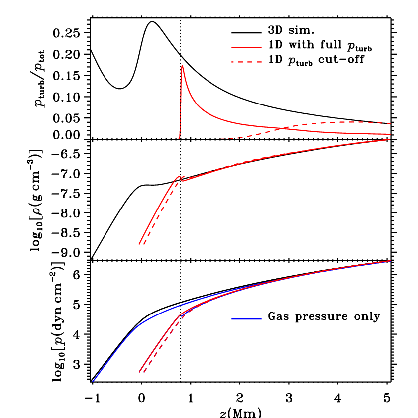
at the surface causes a gas pressure inversion, not seen in the simulations, as well as a much increased density inversion. To include this full 1D turbulent pressure, we had to limit the form-factor of equation (6) to , as opposed to from the calibration. This is seen in the top panel as a lack of convergence to the 3D result with depth. If a model with the more realistic value of could converge, the turbulent pressure would be the dominant contributor, at 53.4% of the total pressure. The local pressure scale height at the turbulent pressure peak is about 0.8 Mm, and the drop from that peak to zero occurs in under 15% of that. To enable integration of hydrostatic equilibrium, it is therefore necessary to introduce some cut-off for . We have constructed this to be smooth and gradual (small gradient) and deep, just above the matching point, minimizing its effect on the models.
In the 3D simulations, on the other hand, turbulent pressure peaks about half a pressure scale height below the top of the convection zone, drops off smoothly both above (from convective overshooting) and below and is non-zero at all depths. The maximum (with depth) of the turbulent to total pressure ratio is shown in Fig. 3 of Trampedach et al. (2013), and that quantity is a good measure of how vigorous the convection is. For the Sun, that ratio is 13.75%.
We recommend not including a 1D-turbulent pressure which is confined to the convection zone, since it will exhibit unphysically large and damaging gradients at the top of the convective envelope (see Fig. 3). Baker & Gough (1979) noted that the turbulent pressure, if included consistently (in all terms), increases the order of the equations for the structure of the envelope model from three to four. They further found that without overshoot the transition to the non-convective case at the boundaries of the convection zone gives rise to singularities which have proved very difficult to treat numerically. Most non-local and/or time-dependent, MLT-style descriptions of convection also accommodate overshooting (Spiegel, 1963; Shaviv & Salpeter, 1973; Nordlund, 1974; Ulrich, 1976; Gough, 1977; Eggleton, 1983; Grossman, 1996; Grigahcène et al., 2005), and some of these have the correctly negative convective flux in the overshoot region. Most of these still have a strong and direct connection between velocities and fluxes, meaning that the velocities still fall off to sharply, producing unphysically large gradients in turbulent pressure, or alternatively, producing too extended a flux transition from convection to radiation (see also Renzini, 1987, for further analysis). The reason for this is the assumed constancy of the fractional area occupied by each direction of convective flows, and , and the often assumed symmetry of these: . Some of these models have positive convective fluxes in the overshoot region because they mainly consist of a smoothing of quantities over some length scale. In our simulations the negative convective overshoot flux is due to a reversal in temperature change in response to a radial displacement, with the upflows getting cooler than the downflows. Our simulations do not address the issue of overshooting at the bottom of convective envelopes, but one could argue that a successful model for overshooting should also be able to reproduce, at least qualitatively, our results for overshoot into the atmosphere. Overshooting from convective cores and the bottom of convective envelopes is crucial for various stages of stellar evolution and an improved understanding is much needed.
Well below the super-adiabatic top of the convection zone, does match the turbulent pressure of the simulations rather well, giving an almost differentiable match. This is part of our evidence that envelope models including , with and fitted as described in Sect. 5, give a realistic extension of the simulations towards the centre of the star. This fact was exploited in an investigation of convective effects on the frequencies of solar oscillations (Rosenthal et al., 1999) by analysing eigenmodes in a model combining the simulation and a matched envelope model. This same procedure was also employed in a calculation of p-mode excitation (Stein et al., 2005; Stein et al., 2007) for a range of stars. We can now proceed with the matching, with confidence.
5 Matching to envelope models
In order to derive values from the simulations we matched 1D envelope models to horizontal and temporal averages of the 3D simulations at a common pressure point deep in the simulation. The matching is performed by adjusting , equation (6), until the 1D-turbulent pressure agrees with that of the simulation, and until the temperatures agree, while keeping the mass and luminosity of the envelope constant. The masses, as listed in Table 1, are chosen based on the atmospheric parameters of evolution tracks constructed with the MESA-code (Paxton et al., 2011), calibrated to the present Sun as per usual (Gough & Weiss, 1976). The luminosity follows from this mass and the atmospheric parameters of the simulations. These masses are obviously inconsistent with our calibration, but our calibration is also insensitive to this choice of mass, with .
This method demands a high degree of consistency between the simulations and the envelope models at the matching point, which is the reason for using the exact same EOS (and chemical composition) in both cases, and for including a turbulent pressure in the deep part of the envelope models. The depth of the matching point is chosen for each simulation as a trade-off between minimizing boundary effects (which increase with depth), and minimizing fluctuations in thermodynamic quantities (which decrease with depth). The latter is to ensure that the mean , and are related by the EOS, i.e., that direct 3D-effects are negligible, as is of course always the case in 1D models. In all our cases, the matching point is located deeper than , and at pressures at least 100 times larger than in the photosphere.
In order to filter out non-convective effects from this calibration of , we also demand consistency between 1D and 3D in the treatment of radiative transfer in the atmosphere. We accomplish this by using the Rosseland opacities and the relations from the 3D simulations, in the atmospheres of the 1D envelope models (see Paper I for details).
We also note that the common pressure point between the averaged 3D simulation and 1D model, being located deep in the simulation, means that the two models generally will disagree on the location of the surface, , of the star (where ). This is due to the convective expansion of 3D atmospheres compared with 1D, as discussed by Trampedach et al. (2013). The 1D envelopes therefore have slightly smaller radii (by up to a per cent of the stars radius for the warmest giant and by as little as for the coolest dwarf), and hence slightly larger and , when the 3D simulation and 1D envelope are constrained to have identical mass and luminosity.
The main advantage of our method for calibrating the MLT is the resulting combined models of averaged 3D simulations outside the matching point and the calibrated 1D envelope model interior to the matching point. Our method ensures these combined models are continuous, and they can therefore be used for computing various asteroseismic quantities, which can then be interpolated in the grid of simulations. Such combined models have been used by Rosenthal et al. (1999) to estimate the helioseismic surface effect, i.e., systematically overestimated model frequencies due to shortcomings at the surface of 1D solar models. They have also been employed in a calculation of p-mode excitation for a range of stars (Stein et al., 2005; Samadi et al., 2007; Stein et al., 2007), based on the formulation by Nordlund & Stein (2001); Stein & Nordlund (2001). Such calculations are also planned for our grid of simulations and calibrated 1D models presented here. The method used by LFS, of matching to the entropy of the adiabat, does not ensure such continuous matching of 1D interior and averaged 3D atmospheres and complicates their use for asteroseismic applications. Their method does, however, ensure the correct location of the bottom of the convective envelope as determined by the Schwarzschild criterion. The two methods will converge with deeper matching point of our method, as the stratification approaches the adiabat exponentially.
6 Results
In Fig. 4 we show the results of this calibration of the MLT as function of effective temperature and gravity. The corresponding atmospheric entropy jump is shown in Fig. 4 of Trampedach et al. (2013). We also list these calibrated values in Table 1 together with their standard deviations, from performing the envelope matching to individual time-steps of the horizontally averaged simulations. This scatter in ranges between 0.015 and 0.040, with an average of 0.026. The standard deviations listed for is likewise from the fluctuations in time. In Table 1 we also list the resulting depths of the convective envelopes, , relative to the stellar radii.

In Fig. 5 we show our calibrated values as function of , with error-bars corresponding to the RMS scatter in and . The local -gradient of is indicated with line-segments,
Our calibration results in low values along the warm edge of our grid, which is approaching the end of convective envelopes from the cool side of the HR diagram. The depth of convective envelopes decreases as this edge of our grid is approached, as does the convective efficiency, quantified by . The highest values are found in the coolest dwarfs, spanning the range from to 2.05 on the main sequence. A 0.7 M⊙-star would experience the largest change in over its life-time (about 0.15), whereas 0.8–1.1 M⊙ stars find themselves on a triangular plateau of , spanning a temperature range of –6 000 K along the main sequence and going up to . This feature was also noted by LFS. This plateau encompasses the evolution so far of the Sun, as well as the nearest and best constrained binary, Cen A and B (the C component is too cool to be covered by our grid of simulations), which means that the evolution of these three stars is well described by a single value of (range, uncertainty of calibration).
Stars ascending the giant branch essentially follow iso- curves, so here is a function of mass and approximately constant with age. The values here range from 1.56 for a 4.3 M⊙-star to 1.75 for 0.84 M⊙. Stars more massive than about 1.25 M⊙ experience a significant increase in during their evolution, but most of that change occurs in the Hertzsprung gap of fast evolution. Effectively they have a small on the main sequence and a larger on the giant branch. Bear in mind, however, that our grid of simulations only covers up to 1.4 M⊙ on the main sequence.

6.1 Comparison with Ludwig, Freytag & Steffen (1999)
The calibration of against 2D RHD simulations performed by LFS employed a method completely independent of ours. In Fig. 5 we have displayed their fit to their results, as applied to the atmospheric parameters of our simulations (lower set of blue ’s, with line-segments indicating their local -derivatives). They suggest a scaling of their results by 1.1–1.2 to translate from 2D to 3D, and we note the profound morphological differences between 2D and 3D atmospheric convection, as discussed by Asplund et al. (2000). LFS also recommend that in order to match 1D solar structure models to the present age Sun, modellers should use the LFS calibration differentially, scaling it by their . We fully adopt that recommendation, with the caveat that the relations and atmospheric opacities of the 3D simulations should be used alongside our calibration. We expect this procedure to result in a minimal need for scaling, but would be most interested in hearing of contrary experiences.
Our results do indeed agree with LFS’s in the solar vicinity, after a scaling by 1.11, as shown by the upper set of red diamonds in Fig. 5. The disagreement around K is most likely also due to differences in the opacities. They based their opacities on the Atlas6 line opacities whereas we use the somewhat newer Atlas9 line opacities (in the form of opacity distribution functions). The difference, as outlined by Kurucz (1992c), consists of the addition of molecular opacity (hydrides and CN, C2 and TiO) and improved calculations for the iron-group elements – all in all a factor of 34 more molecular, atomic and ionic lines.

These opacity changes should affect the hotter stars the least, but they still have an effect on the solar model – that was, after all, the main motivation behind the opacity updates (Kurucz, 1992b). We therefore suspect that the scaling factor, translating LFS’ results from 2D to 3D should be based on the hotter stars. But there are also other differences between our simulations: LFS used grey radiative transfer in the bulk of the 58 2D simulations going into their analysis, adding another systematic difference (also generally decreasing with ) between our results. Furthermore, they used the old pre-helioseismology value of the helium abundance, %, which effectively lowers the atmospheric opacity, compared with ours (the He, being an inert gas, displaces high opacity species, as well as electron donors for H- formation).
The ratio between the two calibrations is also shown in an atmospheric HR diagram in Fig. 6, which also shows the extent of LFS’s grid. From this plot it is clear that most of our simulations have values exceeding those of LFS’s 2D simulations, except for giants with . Our warmest giant has but is also an extrapolation from LFS’s grid. The maximum, for our warmest dwarf which is also within their grid, is 1.27.
It seems natural to expect that quantities other than and would be more relevant for describing the efficiency of convection. The optical depth at the top of the convection zone, for example, seems much more relevant and directly related to the issue, or the peak amplitude of the turbulent to total pressure ratio, or the Mach number as suggested by Samadi et al. (2013). These quantities as well as others we have tested, do not provide simpler or single-valued functions for , and the scatter is large than the individual . We conclude that two independent variables are necessary to describe , and we naturally choose and .
6.2 Gravity darkening of slowly rotating stars
A slowly rotating star can, as a first-order approximation, be described as a set of 1D stellar models with outer boundary conditions that depend on co-latitude, , as and , where is the radius of the star and is the (uniform) rotation rate. A formulation was developed by von Zeipel (1924) for stars in radiative equilibrium, and a main finding22 2 Whether his result is predicated on the assumption that the opacity is of the form (compared with the actual ), is not clear and is beyond the scope of the present work. was that .
Building on this, Lucy (1967) extended the formulation to also apply to convective envelopes, assuming that the various latitudes are connected in the deep convection zone by a common adiabat. The generalisation of von Zeipel’s result is , defining the gravity-darkening exponent . In case of convective envelopes and under the common-adiabat assumption, this gives rise to the adiabatic gravity-darkening exponent
| (7) |
We have evaluated by finding the slopes of the adiabats in Fig. 1, as shown in Fig. 7. The values we find are similar to the value, , which was originally suggested by Lucy (1967), and also agrees with the values reported by LFS although we seem to find a larger range.

The Sun, with an equatorial rotation rate of 450 nHz, displays an equatorial that is a mere dex smaller than at the poles. Making the above assumption of a common adiabat of the deep convection zone, and using from Fig. 7, results in the equator being an unobservable 12 mK cooler than the pole (a contrast of ).
On the other hand, it is also quite likely that meridional flows in stars will build up an entropy gradient with latitude, as suggested by Miesch, Brun & Toomre (2006). If we take a latitude-independent as the other extreme of possibilities, we get an entropy contrast in the solar convection zone of . This is similar to the range of contrasts, 0.95–, explored by Miesch, Brun & Toomre (2006) to obtain the observed solar differential rotation in a 3D simulation of the deep solar convection zone.
Rotational effects are obviously much more important for many other stars. Also in this regard has NASA’s Kepler mission provided a treasure trove of observations, with several recent calculations of rotation periods from spot-modelling of planet candidate host stars by Walkowicz & Basri (2013), McQuillan, Mazeh & Aigrain (2013), of 12 000 other F–M Kepler targets by Nielsen et al. (2013) and of 34 000 Kepler main-sequence targets cooler than 6 500 K by McQuillan, Mazeh & Aigrain (2014) with periods down to 0.2 days.
For fast rotators, more elaborate models are needed [See, e.g., Espinosa Lara & Rieutord (2011) for analytical 2D work and Augustson et al. (2012) for 3D hydrodynamics simulations], but the behaviour of in Fig. 1 should still be relevant for such modelling.
7 Implications for stellar structure
In this section we explore the effects of outer boundary conditions on the 1D structure models, introduced in Sect. 4. We evaluate sensitivities to changes in , relations and atmospheric opacities in Sect. 7.1 and employ the relations of Paper I, together with other commonly used choices, in Sect. 7.2, commenting on the effects on the depths of convective envelopes. This analysis does not include calibrations of , but address how global properties of 1D models react to independent changes to , relation and .
The reason for convection zones growing with increasing convective efficiency, , is found in Sect. 7.4.
7.1 The depth of outer convection zones
The depth of an outer convection zone depends in a complex way on the surface boundary conditions. With some simplifications, however, a rough idea of the mechanisms involved can still be obtained. We convert the equation of hydrostatic equilibrium from the conventional height scale to an optical depth scale
| (8) |
and integrate inward from to get the pressure with depth. For the present discussion we only need the differential response to changes in the atmosphere and the precise values of the quantities are immaterial. We therefore write the pressure in the photosphere
| (9) |
as a one-step numerical integration from to and to , where and are some appropriate averages over the atmosphere. This results in a first-order estimate of the effects of changing various parts of the physics in the atmosphere.
Using some average of the inverse relation for , a relation between and is obtained. An increase in will decrease , as the relation is monotonically increasing, and will therefore have the same decreasing effect on as will an increase in the opacity. Changes to the relation are performed on the generalised Hopf functions, equation (5), which are normalised by the surface flux.
We will now assume that an atmospheric pressure change [due to changes to or ], represents the same factor of pressure change throughout the convection zone. The change in the depth of the convection zone can be derived from the response to such a pressure change at the bottom of the convection zone. The Schwarzschild criterion for convection to occur, equation (1), is mainly governed by , as the adiabatic gradient is very close to the ideal- and fully-ionised-gas value of at the bottom of deep convection zones.
In the deep interior, where the Hopf function, equation (5), is constant and the turbulent pressure is insignificant, the radiative temperature gradient is
| (10) |
This gradient will decrease with a decrease in pressure and the bottom of the convection zone will therefore move outward. Since depends strongly on temperature and has a steep gradient at the bottom of the convection zone, the pressure change hardly affects the location of on the temperature scale. The largest effect is therefore due to the (almost unchanged) temperature at the bottom of the convection zone occurring at a smaller pressure.
This trend is confirmed by the experiments. We calculated envelope models with small (additive) changes (0.005) to , and the atmospheric opacity, in order to find the differential changes to the relative depth (in units of stellar radius, ) of the convection zone. The fundamental parameters, , and (and hence also and ) were held constant between the experiments. Keeping constant effectively anchors the temperature structure so that the effect of the perturbations in , and give similar magnitude responses in and (and close to constant in the convective envelope) and an order of magnitude smaller response in .

The results of these experiments are presented in Figs. 8–10, in the form of changes to the depth of the convective envelope, as function of the atmospheric parameters and . Our experiments shows that both in Fig. 8 and in Fig. 9 are negative and have a similar functional form so that . The depth of the convection zone increases with increasing , as expected (see Sect. 7.4), and we have approximately .

The convective flux in the MLT formulation may be written as
| (11) |
where is the temperature gradient in the upflowing convective elements and is the average of the gradient between the up- and downflowing elements. Note that this is all in the 1D mixing-length picture, so the average gradient , is not the average of a 3D quantity which would have been denoted by . The difference between and is almost equal to the superadiabatic gradient, . Based on equation (11), an increase in temperature and/or a decrease in pressure (brought about by changes to the relation or the atmospheric opacity) will therefore be accompanied by an increase in in order to maintain the total flux (and the fixed of the model). This increase of , corresponding to a decrease of the efficiency of the convection, will lead to a smaller convection zone. The effect can be counteracted by increasing , which increases the convective efficiency by increasing the distance travelled by convective elements. An increase in the efficiency of convection will enlarge the convection zone, as seen from Fig. 10

(see also Sect. 7.4 below).
As far as global observables are concerned, uncertainties in the atmospheric opacities, line-blocking and mismatches between the scale and the grey opacity may be hidden in together with pure convection effects. This is one reason that so many values for the solar can be found in the literature (another reason being the lack of consensus on the values for the auxiliary MLT parameters). As illustrated by Figs. 8–10, such flaws in the treatment of the photosphere will not have the same effect on all stars and an incorrect differential behaviour would be expected from such a solar calibration, masking real convection effects (i.e., an that varies with atmospheric parameters).
Since it is customary to use a solar-calibrated for computing stellar models, we have also computed a set of envelopes with constant , but still using the individual relations. The effect of this is to overestimate the fractional depth of the convection zone of giants by 4–8% and underestimate it for cool dwarfs by about 1%, as shown in Fig. 11. This effect is somewhat counteracted when also keeping the relations constant (scaled solar). The result of Fig. 11 is then further changed by a reduction of along the warm edge of our grid by 1.7% and an increase of by about 5% along the cool edge.

7.2 Effects of changing the relations
Since there currently are a number of schemes for using relations in stellar models, we find it worthwhile to explore the consequences of a few of these. We have kept the opacity and the mixing length, , unchanged in the experiments below.
As mentioned earlier, one of the first solar relations to be published (Krishna Swamy, 1966), is still in wide-spread use in stellar models. Fig. 12 shows the effect of using this relation (scaled to the stellar ) instead of the individual ones found from the simulations.

The effect is largest for a 4.5 M⊙ star on the horizontal branch (HB), or a slightly more massive star approaching the Hayashi line after crossing the Hertzsprung gap, which has its convection zone decreased from 28% to 21% of the stars radius, from employing the Krishna Swamy relation. The smallest effect (apart from the fully convective No. 4) is found in the cool dwarf corner of the HR diagram (simulation No. 36 of Table 1), where the convection zone depth is only decreased from 33.3% to 33.0%. The solar convection zone shrinks from 27.9% to 25.2% of R⊙, from this change.
Another common approximation is to use a scaled solar relation, albeit a more modern one. Using our solar relation from the convection simulations, we find a change somewhat similar to that depicted in Fig. 12, although with half the range and the solar location defining the zero-point; The cool dwarfs get larger convection zones by 0.04 of their radii and the 4.5 M⊙ HB star has its convection zone decreased by 0.018 of its radius.
Many semi-empirical solar atmosphere models do not include the Rosseland optical depth scale, but are only given on the monochromatic 5000 Å, -scale. On the other hand, opacities for stellar structure calculations only include Rosseland averages, but not the 5000 Å opacity. When trying to combine and in the atmosphere of a stellar structure calculation, an obvious inconsistency emerges, which has been largely ignored. Fig. 13 shows to what extent this is a good approximation.

It shows how the depth of convection zones of 1D envelope models changes when using relations from the simulations together with Rosseland opacities. We see that the change is fairly small, mostly well below 1% of the stellar radius, with models more massive than the Sun having deeper convective envelopes when applying a consistent set of relations and opacities. Our solar case has a convection zone deeper by 0.3% of R⊙ with the consistent combination. The one simulation with a fairly large change, 1.4% of its radius, also has the largest -ratio in the photosphere. This ratio only exceeds unity in the photospheres of the stars along the low- border of our grid. This ratio does exceed unity for all the other simulations at some point higher in their atmospheres.
We recommend to use modern relation based on modern opacities, and if possible, using those same opacities in the atmospheres of the stellar structure models. This is both to ensure consistency and in order to try to separate radiative and convective effects. This makes it possible to have the correct behaviour for stars other than the Sun, which still provides the strongest observational constraints for an calibration.
From the above analysis, we have seen how the depth of the convective envelope depends on three parameters of the atmosphere: the mixing length, , the relation and the opacity. Conversely, it is also clear that an inadequate knowledge of relation and atmospheric opacity can be absorbed into , so that different MLT parameters can result in the same overall stellar structure (i.e., result in the deep convective envelope lying on the same adiabat). This is the most likely reason for the variation in the solar-calibrated in the literature. Consistent treatment of the atmosphere will hopefully tighten the range of .
7.3 Calibrating with fixed relation
In many cases stellar models are computed using scaled solar relations; this includes many of the calibrations against observations discussed below (see Sect. 8.2). We therefore performed such a calibration, based on a fit to the quiet-Sun stratification of the semi-empirical atmosphere model of Vernazza, Avrett & Loeser (1981), referred to as VAL-C.

This choice of relation is the default in, e.g., the ASTEC stellar structure code (Christensen-Dalsgaard, 2008) and the closely related stellar envelope code employed here. ASTEC is also part of the Asteroseismic Modeling Portal (AMP) by Metcalfe, Creevey & Christensen-Dalsgaard (2009). AMP was used for the the seismic calibrations of Mathur et al. (2012), Bonaca et al. (2012) and Metcalfe et al. (2014). For this experiment only, we use the envelope code with its default choice of relation.
In Fig. 14 we show the differences in between this calibration with fixed relation, and our full calibration with individual relations from the simulations (Sect. 6 and Fig. 4). In both cases the calibrations are performed as outlined in Sect. 5, the only difference being the choice of relation. We note that with the VAL-C atmosphere, calibrates to systematically larger values than in the full calibration, except for our coolest dwarf simulation (No. 36 of Table 1). For that case is 0.41 smaller. This is a robust result. We have traced this change of sign and magnitude of ’s sensitivity to the relation, to a an extended overlap of the photosphere and the top of the convection zone in the envelope model. The convective flux increases from 3.2% to 28% of the total flux, at between the two coolest dwarf simulations in our grid. Constructing 10 envelope models, with parameters linearly interpolated between the two calibrated models, we find a continuous, but rapid increase of the photospheric convective flux fraction towards lower . At the increase is from 6.7% to 43%. The consequence is that the relation very directly determines the adiabat of the convection zone of the coolest dwarf, whereas the warmer models have the structure effects of the relation diminish with depth, before appreciable convection is reached. We have further attributed the outward migration of the convection zone to the effect of H2 dissociation on , which for this cool dwarf model is suppressed from its fully ionised value of 2/5 to 0.095 centred at and a value of 0.23 at . The outward decrease in induces a shoulder in , increasing in amplitude as the H2 feature in moves inward with decreasing . This extension of convection into the photosphere by H2 dissociation, was also found by Nordlund & Stein (2001).
We also see this phenomenon in our 3D simulation, with similar behaviour of and a corresponding shoulder on . In 3D the feature is smoothed, compared with the 1D model, by the convective fluctuations. The effect is therefore not due to the atmospheric simplifications of 1D models; rather its physical reality is supported by our 3D simulations.
The effect of the difference in relation is to increase the overall density of the 1D envelope by about 0.1 dex, translating into the large difference in . For all the other cases, the resulting change in interior density is small and negative. We have not yet found the underlying reason for this difference. For our solar case, is 0.09 larger than the calibration with its own 3D relation. The difference is a minimal 0.013 for our K giant (simulation No. 2 of Table 1) and largest for the simulations with around 6 400 K, as well as for the next coolest dwarf (simulation No. 37 of Table 1).
7.4 Is always positive?
An analytical analysis of was carried out by Christensen-Dalsgaard (1997) (hereafter C-D97). His analysis was concerned with a highly simplified but instructive model: approximating the convective envelope with a mass-less (assuming all the stellar mass resides in the radiative interior) polytrope of index , which relates pressure, , to density, , through . Further assuming hydrostatic equilibrium and a fully ionised perfect gas, he obtained the differential of the stellar radius, , (C-D97 equation [9])
| (12) |
where 33 3 Note that C-D97 used the symbol for the absolute depth of the convection zone, whereas we use it for the relative depth. Compared with his equations, all occurrences of are therefore multiplied by ( is unchanged). is the radius of the bottom of the convection zone and is the pressure scale height at . Using C-D97’s equation [6] we define
| (13) |
which contains the temperature and pressure derivatives of the Rosseland opacity,
| (14) |
at . With equation (13) we can eliminate the pressure, , in equation (12) and using C-D97’s equation [15]
| (15) |
where is the specific heat at constant pressure at , we arrive at
| (16) |
is the change of specific entropy from the entropy minimum at the top of the convection zone, and down to the adiabatic part, integrating over the peak in the superadiabatic gradient near the surface. This entropy change is positive according to the Schwarzschild criterion for convective instability, equation (1).
For the location of the bottom of the convection zone, C-D97 found
| (17) |
Combining equations (16) and (17) with , and
| (18) |
we finally obtain
| (19) |
In order for this to be positive, we therefore require the curly bracket to be positive. This can be recast into the surprisingly simple inequality
| (20) |
(assuming that ) and the opposite inequality for .
Under which circumstances do we have ? From equation (13) we find that this is the case when
| (21) |
At the bottom of convective envelopes this is often fulfilled since is negative and of large absolute value and is positive and small, so that the right-hand side of equation (21) will not be much larger than 1. In the solar case, with and we get 1.22, which indeed is smaller than the fully ionised, ideal gas value of .
The bottom of a convective envelope occurs where the radiative temperature gradient drops below the adiabatic temperature gradient [cf. equations (1) and (10)]. Assuming that the convective envelope is not deep enough to reach into the core (in which case the assumptions of mass-less envelope and constant luminosity would break down), the drop in will be due to a decrease in opacity. We therefore expect a large and negative . The pressure dependence of the opacity is generally much weaker than the temperature dependence, and it is in general positive. The criterion for the depth of a convective envelope to increase with , will therefore in general be that of equation (20), which is fulfilled for all the stars considered in the present paper. In particular, for the Sun the above analysis results in . Despite the differences in the two methods; analytic versus numerical and simplified full stellar model versus detailed, but truncated envelope models, this value is close to our result, .
8 Observational constraints
8.1 Depth of the solar convection zone
One of the simulations in our grid, No. 30, corresponds to the Sun, and we have carefully adjusted the entropy of the inflowing gas (a constant) to obtain an effective temperature of K, in agreement with that derived from total solar irradiance (TSI) observations: K, (Willson & Hudson, 1988). A recent, but contentious, reassessment by Kopp & Lean (2011) of a number of space-based, TSI measurements, find a significantly lower quiet-Sun TSI of W m-2, corresponding to K. This is, however, well inside the RMS-scatter of our solar simulation. The composition of this simulation is % and %, as for the rest of the grid, and as detailed in Sect. 3. This is very close to the % and % composition of the present day convection zone of model S (Christensen-Dalsgaard et al., 1996).
Matching this simulation to an envelope-model gives , and a depth of the solar convection zone, R⊙. This is within a mere 2.5 of the value inferred from inversion of helioseismic observations: R⊙ (Christensen-Dalsgaard, Gough & Thompson, 1991) and R⊙ (Basu & Antia, 1997). It is interesting to note that the that results from our calibrated is only a little deeper than the R⊙ found by, e.g., Serenelli et al. (2009), from matching L⊙ and R⊙ of models based on the Asplund et al. (2009) abundances. The uncertainties that we quote for our results are the RMS scatter resulting from performing the full fitting of relations and envelope-matching for the individual time-steps of the relaxed and horizontally averaged simulation. No attempt at accounting for systematic effects has been carried out here.
As indicated below equation (4), there are two more parameters to standard MLT: and . These MLT-parameters and are not linearly independent and we therefore limit ourselves to add to our discussion, keeping . As stated earlier, the calibration presented here, does not reproduce the atmospheric structure of the 3D simulations, it is rather constructed to reproduce the structure inside the chosen matching point. That means the extra free parameter of MLT can be used for matching some other feature of the 3D simulations. We choose the height of the super-adiabatic peak, and the amplitude of super adiabaticity at the matching point, as two illustrative examples.
Fitting with respect to the height of the super-adiabatic peak we get , and , resulting in R⊙, also about 2.5 shallower than inferred from helioseismology. The peak in the super-adiabatic gradient is increased from 0.554 in our standard calibration, to 0.695 with this new value of .
If on the other hand we adjust the form factor, , so as to obtain the same at the matching point, then we get , and , and a R⊙, 1.7 shallower than the helioseismic result. However, the peak of the super-adiabatic gradient becomes nonphysically large, reaching a value of 2.154, about 100 km below the photosphere. This is 3.1 times larger than what we find in the solar simulation and even more than twice as large as the super-adiabatic gradient averaged over only the upflows in the simulation.
That , and cannot be simultaneously matched at a common pressure-point (with plausible parameters), indicates that the MLT formulation converges slowly, if ever, towards the super-adiabatic gradient, , of a real convective envelope. This might be due to the neglect of kinetic-flux in the MLT formulation, as discussed in Sect. 2.
Notice that the depth of the solar convection zone, as found above, results from ab initio calculations, from the EOS and opacity calculations, to the RHD simulations. Apart from the defining parameters (surface gravity, entropy of the inflows at the bottom, and the composition), the adjustable parameters that enter the simulations are the resolution, the viscosity coefficients, and the size of the time step relative to the Courant time. These are tuned to resolve the thermal boundary layer at and the convective structures, to minimize numerical diffusion while avoiding numerical noise, and to minimize the computing time against accuracy. None of these are adjusted to fit solar observations and these parameters are therefore not “adjustable parameters” in the conventional sense. In particular, no parameters have been adjusted to obtain a certain atmospheric entropy jump, or by implication, a certain mixing length, . The close agreement with helioseismology is therefore very encouraging.
We also note that the calibration is insensitive to the new abundances by Asplund et al. (2009), since these differ by having lower C, N and O abundances than what we employ, whereas the Fe abundance is unchanged. The latter greatly affects the solar atmosphere, but C, N and O provide little opacity here, and have little effect on the solar surface layers. The calibration is performed entirely on quantities that are minimally affected by such abundance differences, and in a region of each model with minimal sensitivity to these differences. The translation to a depth of the convective envelope, however, depends on the opacity at the bottom of the convection zone which has major contributions from oxygen (Badnell et al., 2005).
8.2 Some calibrations against stellar observations
There are several semi-empirical calibrations of the mixing length, based on stellar evolution calculations of binaries or stellar clusters, solving for a common age of the stars under the observational constraints. These cannot be compared directly with each other or with our work, since they will depend on details of the adopted convection formulation and treatment of the outer boundary condition, as discussed in Sect. 7. It is, fortunately, a widespread practice to also provide of a solar model calibrated to the present radius and luminosity (Gough & Weiss, 1976), and the differential behaviour with respect to the Sun should be much more robust. In the following, we therefore compare with our results scaled to the of each study, as well as with our unscaled results.
In such a semi-empirical calibration of the Cen system, Morel et al. (2000) found 1.86,1.97), whereas we find values for the two components of and , respectively (No. 24 and 34 in Table 1 and Fig. 1). Yıldız (2007) found that values of 1.64 for the primary and 1.58 for the secondary can reproduce both classic and seismic observational constraints. These are all shown in the right-hand-side of Fig. 15d. We notice that the results of Morel et al. (2000) decrease with , ours are both indistinguishable from the solar value, and those of Yıldız (2007) increase with . The latter have no error bars, but we have assigned a based on the scatter in between the models used for his analysis. The absolute values of different mixing-length calibrations are not expected to agree, since they depend on details in the modelling of the atmospheres. The differences between the two components should be more reliable, though, and we note that all three calibrations can be brought to overlap when each pair is allowed to shift vertically. Also note, however, that only the results of Morel et al. (2000) overlap with their solar-calibrated (same value for those two calibrations) shown with black dotted line.
Stassun et al. (2004) performed a calibration on a pre-main-sequence (PMS) eclipsing binary in Orion, V1174 Ori. Their observations and analysis favour inefficient convection of about (compared with their ) in the pair. This is also supported by the only 0.2-0.3 dex depletion of lithium in the 1.01 M⊙ primary component, while the 0.73 M⊙ secondary displays more than 1 dex depletion. These values do not agree with our calibration, however, where the primary should have . The secondary lies 600 K outside our grid, along a steep gradient, and we attempt no extrapolation. The nearest point in our grid has . Stassun et al. (2004) kept identical for the two components, which might account for some of their problems fitting both stars to the same PMS evolution calculations.

By matching observed and model properties Fernandes et al. (1998) found that three sets of nearby visual binaries could all be described with a solar mixing length of . Within the error-bars, this is consistent with our calibration, although we would expect larger values for the cooler secondary components, as shown in Fig. 15b. Fernandes, Morel & Lebreton (2002) studied the visual binary 85 Peg and found and , compared with their solar value of 1.9. This last result is in excellent absolute agreement with ours, and , as shown in Fig. 15a.
Chieffi, Straniero & Salaris (1995) calibrated against Galactic globular clusters, by either calibrating the temperatures of the red-giant branches (RGBs) or the slope of the main sequences. This latter method depends on being constant in and , from the faint end of the main sequence to 2 mags below the turn off. They divided their results into two metallicity groups, Fe/H and , both with statistically insignificant differences between the main sequence and the red-giant branch, but a tentative increase with metallicity. The lack of change between the MS and the RGB, along with the location of Gyr isochrones, agrees with the triangular plateau we find in our calibration for solar metallicity. Their results of , and is consistent with a linear increase with metallicity, assuming similar behaviour with and at all metallicities.
Fitting to observed RGBs of 28 Galactic globular clusters as function of metallicity in the range Fe/H, Ferraro et al. (2006) found that the Sun and the RGB could be modelled with a common mixing length of 2.17, independent of metallicity. This followed from using the classic Anders & Grevesse (1989)-abundances with . Using instead the more modern abundances of Lodders (2003), with , they found and , likewise independent of metallicity, as shown in Fig. 15d. This result contradicts the findings of Chieffi, Straniero & Salaris (1995) mentioned above. Our results for this case are extrapolations to both lower and , so they should be interpreted with caution. This particular extrapolation almost follows the contours of , though, making the extrapolation less suspect. The extrapolation in metallicity is potentially a bigger issue, but the apparent lack of metallicity dependence of their results, warrants a comparison with our [Fe/H]=0.0 grid.
Piau et al. (2011) studied the red (cool) edge of the RGB, based on a sample of 38 nearby Galactic disk sub-giants and giants with interferometrically determined radii. They find that the red edge, constrained by six stars, is best fitted with compared with their solar calibration of . They also find that a single value fits the observations over a decade of luminosity, in agreement with our calibration showing RGB evolution along contours of . Our results suggest, however, that , for their mass of 0.95 M⊙, should be only 0.04 smaller than . Their sample is close to solar metallicity, with the spread of the observations around the evolution tracks being accounted for by the metallicity effect on the stellar models.
Studying binaries in the Hyades, Yıldız (2006) found a mixing length that varies a factor of 2.3 over the MS mass-range of 0.77–1.36 M⊙. Our calibration suggests a factor 1.15 variation instead, and in the opposite sense (See Fig. 15c).
With further constraints from asteroseismic observations and analysis Mathur et al. (2012) found ranging from 1.6 to 2.2 for 22 main sequence Kepler targets ranging from 0.8 to 1.3 M⊙. They found a possible increase of with , possibly with a bump around K of amplitude 0.2, but with sizable scatter. Bonaca et al. (2012) similarly found a weak increase with (without a bump, though) and also with and metallicity, [Fe/H], for the main-sequence stars in their sample. Both of these results are contingent on the prescriptions for accounting for the surface effect: the systematic frequency shift between observations and 1D MLT models that signal differences around the upper turning point of the modes (Christensen-Dalsgaard & Thompson, 1997; Kjeldsen, Bedding & Christensen-Dalsgaard, 2008). The surface effect constitutes a sizable systematic effect in both analyses. Recently Metcalfe et al. (2014) analysed 42 Kepler targets including solar-like oscillators, F-stars and subgiants, taking special care to physically constrain the surface effect. They find -values that agree with our calibrations, although the dependency on both and is stronger than ours. The metallicities of their sample ranges from [Fe/H] to +0.5 with an average and RMS-scatter of , as well as a single metal-poor star of [Fe/H]. They find that increases with [Fe/H], and that the behaviour with and does not change significantly when only the solar metallicity, , sub-sample is analysed.
In general, the range of values from our calibration is smaller than what is suggested by the various types of stellar model fitting employed above. This can be due to a number of issues, both in the modelling and in the interpretations of observations. In the former category, any inadequacies or inconsistencies in the treatment of atmospheric opacities and relations will be absorbed into the calibrated values of . In the latter category, the translation between observations (whether photometric or spectroscopic) and is one of the most important. To take the temperature of a star is a non-trivial endeavour, but recent advances have been made by, e.g., Casagrande et al. (2010) and Meléndez et al. (2010) based on observations of solar twins (stars that are spectroscopically and photometrically indistinguishable from the Sun), and by Huber et al. (2012) based on asteroseismic analysis of Kepler and CoRoT observations, coupled with interferometric measurements of stellar radii. These calibrations of the -scale are being used in an absolute calibration of a range of photometric systems, based on synthetic photometry of the grid of simulations that we present here.
The mixing length of stellar atmosphere models has also been calibrated against stellar spectra, which is a profoundly different kind of calibration. Fuhrmann, Axer & Gehren (1993), van’t Veer-Menneret & Mégessier (1996) and Gardiner, Kupka & Smalley (1999) all found that only a small value of can reproduce the shape of solar Balmer lines. This is half of the atmospheric mass mixing length found by Trampedach & Stein (2011), and thus does not reflect the scale of mixing. Nor does it correspond to the entropy jump in the atmosphere, which is effectively the quantity calibrated when observed global properties are fitted with evolution models. Instead it reflects the larger super-adiabatic gradient of the warm granules, which dominate the emergent spectrum, including the Balmer lines, due to their brightness (Asplund, 2005; Trampedach, 2010). The solar Balmer lines have been successfully modelled in NLTE, based on a 3D convection simulation (Pereira et al., 2013), and less successfully with 1D PHOENIX models (Hauschildt, Allard & Baron, 1999, using ) and MARCS models (Gustafsson et al., 2008, using ).
The effects on stellar evolution models, of varying both the relation and according to our simulations, will be addressed in Paper III.
9 Conclusion
We have calibrated the MLT parameter by matching 1D envelope models with 3D RHD simulations, and established a significant variation of with stellar atmospheric parameters and . Our results show a triangular plateau with stretching from the bottom of the red-giant branch at to –4 800 K on the main sequence. A similar plateau was found in the calibration by LFS against 2D simulations. This plateau includes the Sun, as well as the Cen system and their evolution so far. This suggests a common and constant for the evolution from the main sequence of these three stars, but much of the pre-main-sequence evolution would have occurred with higher , as shown in Fig. 4.
As stars ascend the giant branch we see that they evolve largely along contours of constant . During this evolutionary stage decreases with mass, from to M (simulations No. 2 to 3). The largest gradients in occur during the evolution of low mass stars, M⊙, and for higher mass stars, M⊙, crossing the Hertzsprung gap after the turn-off from the main sequence.
Although various values of have been considered in the modelling of stellar evolution, an varying during the evolution of a star has, to our knowledge, not been tried yet. Results of such evolution calculations are presented in Paper III.
In Sect. 7 we investigated how changes to the radiative part of the outer boundary affect the structure of a star, using the depth of the outer convection zone as a global measure. We evaluated the linear response of the change in depth of the convection zone caused by changes in atmospheric opacity, relation and mixing length, respectively. Our analysis in Sect. 7.1 shows that the convection zone is about equally sensitive to the three kinds of changes, and consequently different MLT parameter triplets can easily result in the same global properties of a stellar model. References to a particular mixing length are therefore less useful unless accompanied by references to the atmospheric opacity and relation.
We also compared the effects of various commonly used assumptions about the relation, and concluded that using the old solar relation as given by Krishna Swamy (1966), scaled to the of each star, results in convection zones that are shallower by up to 7% of the radius (see Fig. 12). Using scaled versions of the relation from the solar simulation also introduces systematic effects, causing deeper convection zones in stars cooler than the Sun and shallower ones in warmer stars. Using a 5000 Å relation with a Rosseland opacity has a similar but smaller effect. We recommend a consistent usage of relations and their corresponding opacities in stellar structure and evolution calculations.
We stress that the choice of depends on the choice of atmospheric physics, i.e., relation and atmospheric opacity. Employing the commonly used scaled solar relation will alter the effect of , as shown in Sect. 7.2 and Sect. 7.3. We recommend that our calibrated values be used with the atmospheric opacities and individual relations from Paper I.
As ground-based and especially space-borne asteroseismology with CoRoT and Kepler is now providing strong constraints on the structure of stars other than the Sun, stronger demands are placed on our theoretical models. Keeping our models ahead of the asteroseismic capabilities of the next missions, TESS and PLATO, and the recently launched astrometry mission, Gaia, is a great challenge for the modelling community.
An absolute calibration of the mixing-length parameter, , is the first step towards improving the treatment of convection in stellar structure models. A fundamentally improved formulation of convection is of course desirable, but has proven rather difficult to come by. Various attempts have been made to rectify this situation. Canuto (1992) present a formulation based on fully developed turbulence, which, however, does not account for the steep density gradient and the inherent asymmetry between up- and downflows. Lydon, Fox & Sofia (1992) base their model on 3D hydrodynamical simulations of convection, and this is probably the most promising way forward. A number of approximations render their results less than optimal for the next generation of convection models, however.
With the connection between MLT and realistic 3D convection simulations, discussed in Sect. 2 and by Trampedach & Stein (2011), we find a properly calibrated mixing-length formulation, with the mixing length being proportional to the pressure scale height, to be the best choice for the time being.
Data Retrieval:
A file with the calibrated mixing length parameters and Fortran 77 routines for reading and interpolating the data can be downloaded from: http://cdsarc.u-strasbg.fr/viz-bin/qcat?J/MNRAS/442/805 The data-file contains both the radiative Hopf functions, , as found in Paper I, and the calibrated mixing-length parameter, , as function of atmospheric parameters, and . The URL also contains the routines necessary for setting up and interpolating in the triangulation of the irregular grid of simulations (Renka, 1984). Finally, we also supply a simple user-level function to include in stellar structure codes, which does not require any knowledge of the data or the details of the triangulation.
The OPINT opacity interpolation package can be downloaded from http://phys.au.dk/~hg62/OPINT, together with the atmospheric opacities from our calculation (Paper I, Sect. 3.1), merged with interior OP opacities (cf. Sect. 4).
Acknowledgements
We thank the anonymous referee for helpful comments which have substantially improved the presentation. We are grateful to Werner Däppen for granting us access to the MHD-EOS code and to R. F. Kurucz for providing us with his tables of opacity distribution functions. Funding for the Stellar Astrophysics Centre is provided by The Danish National Research Foundation (Grant DNRF106). The research is supported by the ASTERISK project (ASTERoseismic Investigations with SONG and Kepler) funded by the European Research Council (Grant agreement no.: 267864). We would like to thank the Australian Partnership for Advanced Computations (APAC) for generous amounts of computer time. RT acknowledges funding from NASA grants NNX08AI57G and NNX11AJ36G and from the Australian Research Council (grants DP 0342613 and DP 0558836) RFS acknowledges NSF grant AGS-1141921 and NASA grant and NNX12AH49G. This research has made use of NASA’s Astrophysics Data System Bibliographic Services.
References
- Abbett et al. (1997) Abbett W. P., Beaver M., Davids B., Georgobiani D., Rathbun P., Stein R. F., 1997, ApJ, 480, 395
- Alexander & Ferguson (1994) Alexander D. R., Ferguson J. W., 1994, ApJ, 437, 879
- Anders & Grevesse (1989) Anders E., Grevesse N., 1989, Geochim. Cosmochim. Acta, 53, 197
- Asida (2000) Asida S. M., 2000, ApJ, 528, 896
- Asplund (2005) Asplund M., 2005, ARA&A, 43, 481
- Asplund et al. (2009) Asplund M., Grevesse N., Sauval A. J., Scott P., 2009, ARAA, 47, 481
- Asplund et al. (2000) Asplund M., Ludwig H.-G., Nordlund Å., Stein R. F., 2000, A&A, 359, 669
- Asplund et al. (1999) Asplund M., Nordlund Å., Trampedach R., Stein R. F., 1999, A&A, 346, L17
- Augustson et al. (2011) Augustson K., Rast M., Trampedach R., Toomre J., 2011, J. of Phys. Conf. Series, 271, 012070
- Augustson et al. (2012) Augustson K. C., Brown B. P., Brun A. S., Miesch M. S., Toomre J., 2012, ApJ, 756, 169
- Badnell et al. (2005) Badnell N. R., Bautista M. A., Butler K., Delahaye F., Mendoza C., Palmeri P., Zeippen C. J., Seaton M. J., 2005, MNRAS, 360, 458
- Bahcall et al. (2005) Bahcall J. N., Basu S., Pinsonneault M., Serenelli A. M., 2005, ApJ, 618, 1049
- Baker & Gough (1979) Baker N. H., Gough D. O., 1979, ApJ, 234, 232
- Basu & Antia (1995) Basu S., Antia H. M., 1995, MNRAS, 276, 1402
- Basu & Antia (1997) Basu S., Antia H. M., 1997, MNRAS, 287, 189
- Belkacem et al. (2006) Belkacem K., Samadi R., Goupil M., Kupka F., 2006, A&A, 460, 173
- Böhm-Vitense (1958) Böhm-Vitense E., 1958, Zs. f. Astroph., 46, 108
- Bonaca et al. (2012) Bonaca A. et al., 2012, ApJ, 755, L12
- Canuto (1992) Canuto V. M., 1992, ApJ, 392, 218
- Canuto (2000) Canuto V. M., 2000, A&A, 357, 177
- Canuto & Mazzitelli (1991) Canuto V. M., Mazzitelli I., 1991, ApJ, 370, 295
- Canuto & Mazzitelli (1992) Canuto V. M., Mazzitelli I., 1992, ApJ, 389, 724
- Casagrande et al. (2010) Casagrande L., Ramírez I., Meléndez J., Bessell M. S., Asplund M., 2010, A&A, 512, A54
- Chan & Sofia (1987) Chan K. L., Sofia S., 1987, Science, 235, 465
- Chan & Sofia (1989) Chan K. L., Sofia S., 1989, ApJ, 336, 1022
- Chieffi, Straniero & Salaris (1995) Chieffi A., Straniero O., Salaris M., 1995, ApJ, 445, L39
- Christensen-Dalsgaard (1997) Christensen-Dalsgaard J., 1997, in Solar Convection and Oscillations and their Relationship, Pijpers F. P., Christensen-Dalsgaard J., Rosenthal C. S., eds., Kluwer, Dordrecht, 3
- Christensen-Dalsgaard (2008) Christensen-Dalsgaard J., 2008, ApSS, 316, 13
- Christensen-Dalsgaard et al. (1996) Christensen-Dalsgaard J. et al., 1996, Science, 272, 1286
- Christensen-Dalsgaard & Frandsen (1983) Christensen-Dalsgaard J., Frandsen S., 1983, Sol. Phys., 82, 165
- Christensen-Dalsgaard, Gough & Thompson (1991) Christensen-Dalsgaard J., Gough D. O., Thompson M. J., 1991, ApJ, 378, 413
- Christensen-Dalsgaard & Pérez Hernández (1991) Christensen-Dalsgaard J., Pérez Hernández F., 1991, in Lecture Notes in Physics, Vol. 388, Challenges to Theories of the Structure of Moderate-Mass Stars, Gough D. O., Toomre J., eds., Springer, Berlin, 43
- Christensen-Dalsgaard & Thompson (1997) Christensen-Dalsgaard J., Thompson M. J., 1997, MNRAS, 284, 527
- Collet, Asplund & Trampedach (2007) Collet R., Asplund M., Trampedach R., 2007, A&A, 469, 687
- Däppen et al. (1988) Däppen W., Mihalas D., Hummer D. G., Mihalas B. W., 1988, ApJ, 332, 261
- Dziembowski, Pamyatnykh & Sienkiewicz (1991) Dziembowski W. A., Pamyatnykh A. A., Sienkiewicz R., 1991, MNRAS, 249, 602
- Eggleton (1983) Eggleton P. P., 1983, MNRAS, 204, 449
- Espinosa Lara & Rieutord (2011) Espinosa Lara F., Rieutord M., 2011, A&A, 533, A43
- Ferguson et al. (2007) Ferguson J. W., Heffner-Wong A., Penley J. J., Barman T. S., Alexander D. R., 2007, ApJ, 666, 261
- Fernandes et al. (1998) Fernandes J. M., Lebreton Y., Baglin A., Morel P., 1998, A&A, 338, 455
- Fernandes, Morel & Lebreton (2002) Fernandes J. M., Morel P., Lebreton Y., 2002, A&A, 392, 529
- Ferraro et al. (2006) Ferraro F. R., Valenti E., Straniero O., Origlia L., 2006, ApJ, 642, 225
- Freytag, Ludwig & Steffen (1996) Freytag B., Ludwig H.-G., Steffen M., 1996, A&A, 313, 497
- Freytag & Steffen (2005) Freytag B., Steffen M., 2005, in The A-Star Puzzle, Zverko J., Žižňovský J., Adelman S. J., Weiss W. W., eds., Symp. No. 224, IAU, Univ. Press, Cambridge, 139
- Fuhrmann, Axer & Gehren (1993) Fuhrmann K., Axer M., Gehren T., 1993, A&A, 271, 451
- Gardiner, Kupka & Smalley (1999) Gardiner R., Kupka F., Smalley B., 1999, A&A, 347, 876
- Georgobiani, Stein & Nordlund (2003) Georgobiani D., Stein R. F., Nordlund Å., 2003, ApJ, 596, 698
- Gong, Däppen & Zejda (2001) Gong Z., Däppen W., Zejda L., 2001, ApJ, 546, 1178
- Gough (1977) Gough D. O., 1977, ApJ, 214, 196
- Gough & Weiss (1976) Gough D. O., Weiss N. O., 1976, MNRAS, 176, 589
- Grevesse & Sauval (1998) Grevesse N., Sauval A. J., 1998, Space Sci. Rev., 85, 161
- Grigahcène et al. (2005) Grigahcène A., Dupret M.-A., Gabriel M., Garrido R., Scuflaire R., 2005, A&A, 434, 1055
- Grossman (1996) Grossman S. A., 1996, MNRAS, 279, 305
- Gustafsson et al. (2008) Gustafsson B., Edvardsson B., Eriksson K., Jørgensen U. G., Nordlund Å., Plez B., 2008, A&A, 486, 951
- Hauschildt, Allard & Baron (1999) Hauschildt P. H., Allard F., Baron E., 1999, ApJ, 512, 377
- Henyey, Vardya & Bodenheimer (1965) Henyey L., Vardya M. S., Bodenheimer P., 1965, ApJ, 142, 841
- Houdek & Rogl (1996) Houdek G., Rogl J., 1996, Bull. Astron. Soc. India, 24, 317
- Huber et al. (2012) Huber D. et al., 2012, ApJ, 760, 32
- Hui-Bon-Hoa et al. (2002) Hui-Bon-Hoa A., LeBlanc F., Hauschildt P. H., Baron E., 2002, A&A, 381, 197
- Hummer & Mihalas (1988) Hummer D. G., Mihalas D., 1988, ApJ, 331, 794
- Iglesias & Rogers (1996) Iglesias C. A., Rogers F. J., 1996, ApJ, 464, 943
- Kim et al. (1996) Kim Y.-C., Fox P. A., Sofia S., Demarque P., 1996, ApJ, 461, 499
- Kjeldsen, Bedding & Christensen-Dalsgaard (2008) Kjeldsen H., Bedding T. R., Christensen-Dalsgaard J., 2008, ApJ, 683, L175
- Kopp & Lean (2011) Kopp G., Lean J. L., 2011, Geophys. Res. Lett., 38, L01706
- Krishna Swamy (1966) Krishna Swamy K. S., 1966, ApJ, 145, 174
- Kuhfuß (1986) Kuhfuß R., 1986, A&A, 160
- Kupka, Ballot & Muthsam (2009) Kupka F., Ballot J., Muthsam H. J., 2009, Comm. Asteroseism., 160, 30
- Kurucz (1992a) Kurucz R. L., 1992a, Rev. Mex. Astron. Astrofis., 23, 45
- Kurucz (1992b) Kurucz R. L., 1992b, Rev. Mex. Astron. Astrofis., 23, 181
- Kurucz (1992c) Kurucz R. L., 1992c, in The Stellar Populations of Galaxies, Barbuy B., Renzini A., eds., Symp. No. 149, IAU, Springer, Dordrecht, 225
- Lesaffre, Podsiadlowski & Tout (2005) Lesaffre P., Podsiadlowski P., Tout C. A., 2005, MNRAS, 356, 131
- Lodders (2003) Lodders K., 2003, ApJ, 591, 1220
- Lucy (1967) Lucy L. B., 1967, Zeit. f. Astroph., 65, 89
- Ludwig, Freytag & Steffen (1999) Ludwig H.-G., Freytag B., Steffen M., 1999, A&A, 346, 111
- Ludwig & Nordlund (2000) Ludwig H.-G., Nordlund Å., 2000, in Stellar Astrophysics: Proceedings of the Pacific Rim Conference, Hong Kong, 1999, Kluwer, Dordrecht, 37
- Lydon, Fox & Sofia (1992) Lydon T. J., Fox P. A., Sofia S., 1992, ApJ, 397, 701
- Mathur et al. (2012) Mathur S. et al., 2012, ApJ, 749, 152
- McQuillan, Mazeh & Aigrain (2013) McQuillan A., Mazeh T., Aigrain S., 2013, ApJ, 775, L11
- McQuillan, Mazeh & Aigrain (2014) McQuillan A., Mazeh T., Aigrain S., 2014, ApJS, 211, 24
- Meléndez et al. (2010) Meléndez J., Schuster W. J., Silva J. S., Ramírez I., Casagrande L., Coelho P., 2010, A&A, 522, A98
- Metcalfe, Creevey & Christensen-Dalsgaard (2009) Metcalfe T. S., Creevey O. L., Christensen-Dalsgaard J., 2009, ApJ, 699, 373
- Metcalfe et al. (2014) Metcalfe T. S. et al., 2014, ApJS, arXiv:1402.3614, (accepted)
- Miesch, Brun & Toomre (2006) Miesch M. S., Brun A. S., Toomre J., 2006, ApJ, 641, 618
- Militzer & Hubbard (2013) Militzer B., Hubbard W. B., 2013, ApJ, 774, 148
- Morel et al. (2000) Morel P., Provost J., Lebreton Y., Thévenin F., Berthomieu G., 2000, A&A, 363, 675
- Nayfonov et al. (1999) Nayfonov A., Däppen W., Hummer D. G., Mihalas D., 1999, ApJ, 526, 451
- Nielsen et al. (2013) Nielsen M. B., Gizon L., Schunker H., Karoff C., 2013, A&A, 557, L10
- Nordlund (1974) Nordlund Å., 1974, A&A, 32, 407
- Nordlund (1976) Nordlund Å., 1976, A&A, 50, 23
- Nordlund (1982) Nordlund Å., 1982, A&A, 107, 1
- Nordlund & Dravins (1990) Nordlund Å., Dravins D., 1990, A&A, 228, 155
- Nordlund & Stein (1990) Nordlund Å., Stein R. F., 1990, Comput. Phys. Commun., 59, 119
- Nordlund & Stein (1991) Nordlund Å., Stein R. F., 1991, in Stellar Atmospheres: Beyond Classical Models, et al. L. C., ed., Kluwer, Dordrecht, 263
- Nordlund & Stein (1997) Nordlund Å., Stein R. F., 1997, in Solar Convection and Oscillations and their Relationship, Pijpers F. P., Christensen-Dalsgaard J., Rosenthal C. S., eds., Kluwer, Dordrecht, 79
- Nordlund & Stein (2000) Nordlund Å., Stein R. F., 2000, in The Impact of Large-Scale Surveys on Pulsating Star Research, Szabados L., Kurtz D. W., eds., ASP Conf. Ser. 203, IAU Coll. No. 176, ASP, San Francisco, 362
- Nordlund & Stein (2001) Nordlund Å., Stein R. F., 2001, ApJ, 546, 576
- Paxton et al. (2011) Paxton B., Bildsten L., Dotter A., Herwig F., Lesaffre P., Timmes F., 2011, ApJS, 192, 3
- Pereira et al. (2013) Pereira T. M. D., Asplund M., Collet R., Thaler I., Trampedach R., Leenaarts J., 2013, A&A, 554, A118
- Piau et al. (2011) Piau L., Kervella P., Dib S., Hauschildt P. H., 2011, A&A, 526, A100
- Rempel (2004) Rempel M. D., 2004, ApJ, 607, 1046
- Renka (1984) Renka R. J., 1984, ACM Trans. on Math. Softw., 10, 440
- Renzini (1987) Renzini A., 1987, A&A, 188, 49
- Richard et al. (1998) Richard O., Dziembowski W. A., Sienkiewicz R., Goode P. R., 1998, in Structure and Dynamics of the Interior of the Sun and Sun-like Stars, Korzennik S. G., ed., SOHO 6/GONG 98 Workshop, ESA, Noordwijk, 517
- Rieutord & Zahn (1995) Rieutord M., Zahn J.-P., 1995, A&A, 296, 127
- Rogers & Iglesias (1992) Rogers F. J., Iglesias C. A., 1992, ApJS, 79, 507
- Rogers & Nayfonov (2002) Rogers F. J., Nayfonov A., 2002, ApJ, 576, 1064
- Rosenthal et al. (1999) Rosenthal C. S., Christensen-Dalsgaard J., Nordlund Å., Stein R. F., Trampedach R., 1999, A&A, 351, 689
- Samadi et al. (2013) Samadi R. et al., 2013, A&A, 559, A40
- Samadi et al. (2007) Samadi R., Georgobiani D., Trampedach R., Goupil M., Stein R. F., Nordlund Å., 2007, A&A, 463, 297
- Saumon, Chabrier & Horn (1995) Saumon D., Chabrier G., Horn H. M. V., 1995, ApJS, 99, 713
- Seaton (1995) Seaton M. J., ed., 1995, The Opacity Project, Vol. 1. Institute of Physics Publishing
- Serenelli et al. (2009) Serenelli A. M., Basu S., Ferguson J. W., Asplund M., 2009, ApJ, 705, L123
- Shaviv & Salpeter (1973) Shaviv G., Salpeter E. E., 1973, ApJ, 184, 191
- Spiegel (1963) Spiegel E. A., 1963, ApJ, 138, 216
- Stassun et al. (2004) Stassun K. G., Mathieu R. D., Vaz L. P. R., Stroud N., Vrba F. J., 2004, ApJS, 151, 357
- Stein et al. (2007) Stein R. F., Benson D., Georgobiani D., Nordlund Å., 2007, in Convection in Astrophysics, Kupka F., Roxburgh I., Chan K. L., eds., Symp. No. 239, IAU, Cambridge University Press, 331
- Stein et al. (2005) Stein R. F., Georgobiani D., Trampedach R., Ludwig H.-G., Nordlund Å., 2005, in XXVth General Assembly, Engvold O., ed., Highlights of Astronomy No. 13, IAU, ASP, San Francisco, 411
- Stein & Nordlund (1989) Stein R. F., Nordlund Å., 1989, ApJ, 342, L95
- Stein & Nordlund (1998) Stein R. F., Nordlund Å., 1998, ApJ, 499, 914
- Stein & Nordlund (2001) Stein R. F., Nordlund Å., 2001, ApJ, 546, 585
- Stein & Nordlund (2003) Stein R. F., Nordlund Å., 2003, in Stellar atmosphere modeling, Hubeny I., Mihalas D., Werner K., eds., ASP Conf. Ser. No. 288, 519
- Stellingwerf (1976) Stellingwerf R. F., 1976, ApJ, 206, 543
- Tanner, Basu & Pierre (2014) Tanner J. D., Basu S., Pierre D., 2014, ApJ, 785, L13
- Trampedach (2005) Trampedach R., 2005, in The A-Star Puzzle, Zverko J., Žižňovský J., Adelman S. J., Weiss W. W., eds., Symp. No. 224, IAU, Univ. Press, Cambridge, 155
- Trampedach (2010) Trampedach R., 2010, Ap&SS, 328, 213
- Trampedach et al. (2013) Trampedach R., Asplund M., Collet R., Nordlund Å., Stein R. F., 2013, ApJ, 769, 18
- Trampedach et al. (2014) Trampedach R., Christensen-Dalsgaard J., Nordlund Å., Asplund M., Stein R. F., 2014, MNRAS, 442, 805
- Trampedach et al. (1997) Trampedach R., Christensen-Dalsgaard J., Nordlund Å., Stein R. F., 1997, in Solar Convection and Oscillations and their Relationship, Pijpers F. P., Christensen-Dalsgaard J., Rosenthal C. S., eds., Kluwer, Dordrecht, 73
- Trampedach & Stein (2011) Trampedach R., Stein R. F., 2011, ApJ, 731, 78
- Turcotte et al. (1998) Turcotte S., Richer J., Michaud G., Iglesias C. A., Rogers F. J., 1998, ApJ, 504, 539
- Ulrich (1970) Ulrich R. K., 1970, Ap&SS, 9, 80
- Ulrich (1976) Ulrich R. K., 1976, ApJ, 207, 564
- van’t Veer-Menneret & Mégessier (1996) van’t Veer-Menneret C., Mégessier C., 1996, A&A, 309, 879
- Vernazza, Avrett & Loeser (1981) Vernazza J. E., Avrett E. H., Loeser R., 1981, ApJS, 45, 635
- von Zeipel (1924) von Zeipel H., 1924, MNRAS, 84, 684
- Vorontsov, Baturin & Pamyatnykh (1991) Vorontsov S. V., Baturin V. A., Pamyatnykh A. A., 1991, Nature, 349, 49
- Walkowicz & Basri (2013) Walkowicz L. M., Basri G. S., 2013, MNRAS, 436, 1883
- Willson & Hudson (1988) Willson R. C., Hudson H. S., 1988, Nature, 332, 810
- Yıldız (2006) Yıldız M., 2006, MNRAS, 368, 1941
- Yıldız (2007) Yıldız M., 2007, MNRAS, 374, 1264