Exact solution of a (2 + 1) dimensional anisotropic star in Finch and Skea spacetime
Abstract
We provide a new class of interior solution of a (2 + 1) dimensional anisotropic star in Finch and Skea spacetime corresponding to the BTZ black hole. We have developed the model by considering the MIT bag model EOS and a particular ansatz for the metric function proposed by Finch and Skea [1]. Our model is free from central singularity and satisfied all the physical requirements for the acceptability of the model.
pacs
04.40.Nr, 04.20.Jb, 04.20.DwI Introduction
Introduction of lower dimensional gravity, soon became an interesting tool as many difficult fundamental problems of dimensions became much much simpler in dimensions. It did enhance various understandings of gravity theories. Though conventional realization of a black hole was first revealed in the back ground of dimensional space time, a lower dimensional analysis is preferred more to understand the different issues. Banados, Teitelboim and Zanelli (hence BTZ) [2], in the presence of negative cosmological constant, had constructed an analytic solution representing the exterior gravitational field of a black hole in dimensions which was opened up the possibility of investigating many interesting features of black holes. Recently, Rahaman et al [3] have obtained a different kind of exact BTZ black hole solutions of Einstein’s field equations in dimensional anti-de Sitter back ground space-time in the context of non-commutative geometry . R. B. Mann and S. F. Ross had investigated under what circumstances a disk of pressureless dust, actually a 3D analogue of Oppenheimer-Snyder collapse, will collapse to the zero angular momentum BTZ black hole [4]. The properties of such type of collapse found to be the parallel process to the 4 dimensional ones. Collapse to a point singularity occurs in finite proper time, and the event horizon forms in infinite coordinate time, with an infinite redshift. Martins et al [5] considering the collapse of dark energy fluids, had studied the collapse of an anisotropic fluid with zero radial pressure. Irrespective of the initial fluid nature they obtained a black hole as a result(in dimensions). This was significantly different from higher dimensional phantom energy collapse [6]. Cruz and Zanelli[7] obtained an interior solution for an incompressible fluid in dimensions and investigated the bound on the maximum allowed mass of the resultant configuration. By assuming a particular density profile, a class of interior solutions corresponding to BTZ exterior was provided by Cruz et al[8]. Consideration of three-dimensional perfect fluid stars in hydrostatic equilibrium(with polytropic EoS), matched to the BTZ black hole exterior geometry was done by Paulo M. Sa.
The introduction of a negative cosmological constant for stellar solutions with finite mass and finite radius, did match to an exterior black hole geometry in a way similar to the situation in four dimensions. The solution obtained by Sharma et al [9] is regular at the center and it satisfies all the physical requirements except at the boundary where the authors have proposed a thin ring of matter content with negative energy density so as to prevent collapsing. The discontinuity of the affine connections at the boundary surface provide the above matter confined to the ring. Such a stress-energy tensor is not ruled out from the consideration Casimir effect for massless fields.
Derivation of all perfect fluid solutions for the static circularly symmetric space-time was done by Garcia [10]. The general solution is presented in the standard coordinate system , and alternatively, in a system the canonical one with coordinates . The exact analytic form of the metric potentials, in this formulation, can be obtained for any arbitrary choice of the density profile or EOS of the matter content of the fluid source. In particular, they presented a solution corresponding to a static circularly symmetric perfect fluid source having constant energy density, which (in the presence of a cosmological constant) might be considered as analogous to the incompressible Schwarzschild interior solution in dimensions. Since determination of the exact analytic form of the solution in this formalism requires knowledge about the EOS of the composition or the radial dependence of energy-density, we find it worthwhile to adopt an alternative method where the right hand side of the Einstein’s field equations () will be governed by the geometry of the associated space-time ( ).
II Interior Space-time
The metric for a static circularly symmetry Finch and Skea type star in dimensional spacetime can be written as
| (1) |
Where is a curvature parameter and hypersurface of the metric is parabolic in nature.
Let us assume that the energy momentum tensor for the matter distribution at the interior of the star is of the form,
| (2) |
Where and .Here the vector is the fluid velocity and is the spacelike vector which is orthogonal to , is the energy density, and are respectively the radial and the transversal pressure of the fluid. The Einstein field equation in dimension with cosmological constant for the spacetime given in equation together with the energy-momentum tensor given in equation ,assuming gives three independent equations as follows:
| (3) |
| (4) |
| (5) |
Let us consider the equation of state as
| (6) |
where is the Bag constant.
Solving equation and with the help of equation we get,
| (7) |
where is the constant of integration.
The space-time metric thus obtained is free from central singularity.
From equation we get the expression for density as,
| (8) |
Putting the value of in equation and the expression for radial pressure is obtained as,
| (9) |
Using in we get the expression of as,
| (10) |


III Exterior Space-time and Matching condition
Let us match our interior solution to exterior BTZ Black hole metric,
| (11) |
Where the parameter is the conserved charged associated with asymptotic invariance under the time displacements. Let us assume that is the radius of the star.Therefore,by the continuity of the metric function and at the boundary of the star we get,
| (12) |
and
| (13) |
Now at the boundary the pressure is zero ,i.e, which gives,
| (14) |
Solving equation and we get,
| (15) |
Which gives the value of the curvature parameter governing the value of the curvature spacetime of the metric given in equation and
| (16) |
which gives the value of Bag Constant.
Putting the values of and in equation one can easily obtain the value of integration constant . Let us take the value of and and radius of the star .Then from equation we get and from equation we get . Note that while solving Einstein’s equations as well as for plotting, we have set c=G=1. However, if you keep these parameters from the beginning, the central density in our case turns out to be . The Bag constant will be . Plugging G and c into relevant equations, the value of the central density and Bag constant turn out to be and .
IV Physical Condition
For a physical meaningful solution we must have density and pressure are decreasing function of . In our model,from equation and ,we have,
| (17) |
| (18) |
At the point
and
Which shows that density and pressure are decreasing function of and they have maximum value at the center and decrease radially
outwards which have been shown in FIG. and FIG. respectively.
Now central density is obtained as,
| (19) |
and radial and transverse pressures at center are obtained as,
| (20) |
These show that density and radial pressure both are regular at the center of the star. We have plotted density and radial
pressure in FIG. and FIG. respectively. The figures indicate that density and pressure both are positive inside the stellar object.
The equation of state parameters and are given by the equations
| (21) |
| (22) |
We plot these parameters in and respectively. One can note that radial EoS parameter lies within , however, transverse EoS parameter increases with radial distance gets the value which is greater than unity.
The measure of anisotropy is given by,
| (23) |
We have plotted the measure of anisotropy in FIG.. Figure indicates that the anisotropy is directed outwards.


Now at the point which gives the physically meaningful solution.
We must have for appropriate signature of the metric. This gives,
| (24) |
Therefore, we get an upper bound of from equation .
V Energy Condition:
It is well-known that that the null energy condition (NEC),weak energy condition(WEC) and the strong energy condition (SEC) will be satisfied if and only if the following four equations holds simultaneously at every point within the source:
| (25) |
| (26) |
| (27) |
| (28) |
Employing all the energy condition at the center We note that the first condition will be satisfied if
The second condition will be satisfied if
The third condition will be satisfied if
The fourth condition will be satisfied if
The assumed and estimated values of are consistent with the equations at the origin. We have plotted the L.H.S of equations in and from the figure it is clear that all the energy conditions are satisfied.

VI Some Features:
VI.1 Mass Radius Relation
The mass function of the stellar object within the radial distance is given by,
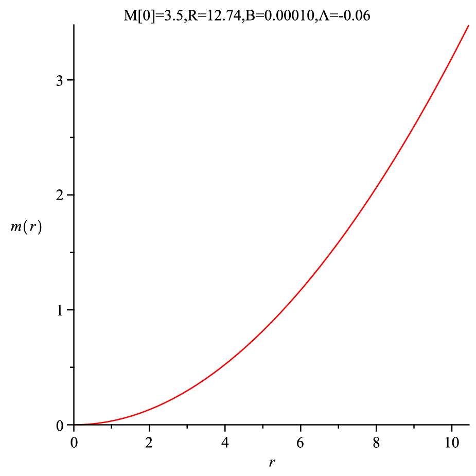
By using equation the upper limit of mass may be written as
| (29) |
which gives,
VI.2 Compactness:
The compactness of the stellar configuration is given by
| (30) |
To see the maximum allowance of the mass radius
ratio of our model we have plotted in
FIG.. From the figure, we notice that is an
increasing function of ’r’ and the maximum value of
is . Thus ratio lies within the standard limit of (3+1) dimensional case.

VI.3 Surface Redshift:
The surface red shift function is given by
| (31) |
Which has been shown in figure . The maximum redshift of our (2+1) dimensional star of radius 10.45 turns out to be 0.729.

VII TOV Equation
The Generalized Tolman-Oppenheimer-Volkoff (TOV) equation is of the form [11]
| (32) |
where is the gravitational mass within the radius and is given by,
| (33) |
Substituting the value of in equation we get,
| (34) |

The TOV equation in equation described the equilibrium of the stellar configuration under gravitational force ,hydrostatic force and anisotropic stress within the stellar object so that
| (35) |
where
| (36) |
| (37) |
| (38) |
In figure we have plotted and for a particular stellar configuration. The figure indicates that the star is in static equilibrium under these three forces.
VIII Discussions
We have presented a new class of solution in anisotropy corresponding to the BTZ exterior spacetime in dimensional Finch and Skea spacetime . Our solutions are regular at center and satisfy all the physical requirements .We have obtained the upper bound of the mass function. It was proved by Buchdahl that for maximally allowable mass-radius ratio for (3+1) dimensional spacetime. For our model the maximally allowable mass radius ratio is which lies within the standard limit of (3+1) dimensional case. Estimated value of Bag constant is 60-80 Mev for a equilibrium stable strange matter configuration [12, 13]. Plugging G and c into relevant equation the value of the Bag constant turns out to be B=83.7 Mev which is very close to the accepted value. However, one concern of this model is the transverse pressure. It increases with radial distance as well as transverse EoS is greater than unity. This behavior is shown due to high compactness of the ultra-compact star where the density is above the nuclear density.
IX Acknowledgements
FR and RB would like to thank the Inter-University Centre for Astronomy and Astrophysics (IUCAA), Pune, India, for research facility. FR is also grateful to UGC, Govt. of India, for financial support under its Research Award Scheme. PB is thankful to CSIR, Govt. of India for providing JRF. RB thanks CSIR for awarding Research Associate fellowship.
References
- [1] M. R. Finch and J. E. F. Skea, Class. Quantum. Grav. 6 467 (1989)
- [2] Banados, M., Teitelboim, C., Zanelli, J. :- Phys. Rev. Lett. 69, 1849 (1992).
- [3] F. Rahaman, KP. K. F. Kuhfittig, B. C. Bhui, M. Rahaman, S. Ray and U. F. Mondal, Phys. Rev. D, 87, 084014 (2013).
- [4] Mann, R. B., Ross, S. F. :- Phys. Rev. D 47, 3319 (1993).
- [5] Martins, M. R., da Silva, M. F. A. and Sheng, Andrew D. :- Gen. Relativ. Grav. 42, 281 (2010).
- [6] Rudra, P., Biswas, R., Debnath, U. :- Astrophys Space Sci 335 505(2011).
- [7] Cruz, N., Zanelli, J.:-Class. Quantum Grav.12, 975(1995).
- [8] Cruz, N., Olivares, M., Villanueva, J. R.:- Gen. Relativ. Grav. 37, 667 (2005).
- [9] Sharma, R., Rahaman F., Karar, I. :-Phys. Lett. B 704, 1 (2011).
- [10] Garcia A. A., Campuzano,C. :- Phys. Rev. D 67 064014 (2003).
- [11] J. Ponce de León :- Gen. Relativ. Gravit. 25, 1123 (1993).
- [12] M Kalam et al :- Int.J.Theor.Phys. 52 3319-3328 (2013)
- [13] F Rahaman et al :- Eur.Phys.J. C 72 , 2071 (2012)