On the error of incidence estimation from prevalence data

Ralph Brinks
Institute for Biometry and Epidemiology
German Diabetes Center
Düsseldorf Note: ralph.brinks@ddz.uni-duesseldorf.de Germany

Abstract

This paper describes types of errors arising in a recently proposed method of incidence estimation from prevalence data. The errors are illustrated by a simulation study about a hypothetical irreversible disease. In addition, a way of obtaining error bounds in practical applications of the method is proposed.

Keywords: Error; Sampling error; Systematic error; Chronic diseases; Incidence; Prevalence; Mortality; Illness-death model; Ordinary differential equation.

1 Introduction

Recently, we have shown how to estimate the incidence of an irreversible disease by the age-specific prevalence in case the mortality of the diseased and the healthy population are known, (Brinks et al., 2013). The age-specific prevalence can, for instance, be obtained from cross-sectional studies. In (Brinks et al., 2013) one cross-section was used to estimate the incidence of renal failure. The underlying approach had been an ordinary differential equation (ODE) which is valid if the only relevant time-scale is the age of the persons in the considered population. Error considerations have been treated by a bootstrap approach.

Later we have proven that the underlying ODE is a special case of a partial differential equation (PDE) that involves additional time scales, (Brinks, 2013a) and (Brinks & Landwehr, 2014). If we want to use the PDE for estimation of the incidence, at least two cross-sections are necessary, (Brinks, 2013b).

This work deals with incidence estimation from two cross-sections using the PDE approach. It is shown that the incidence estimation is affected by three types of error: (i) a systematic error which is given by the study design (or the available data), (ii) the sampling of the age course, and (iii) by the error attributable to sampling the population. After a short summary of our previous works alongside with an introduction of the notation in this article, an example is presented and the types of error are introduced and examined.

2 Illness-death model

In dealing with the incidence, prevalence and mortality with respect to a disease, it is useful to look at the illness-death model shown in Figure 1, (Kalbfleisch & Prentice, 2012). The transition rates are the incidence rate $i,$ and $m_{0}$ and $m_{1}$ are the mortality rates of the non-diseased and diseased persons, respectively. In general, these rates depend on calendar time $t$ , age $a$ and in case of $m_{1}$ also on the duration $d$ of the disease.

Refer to caption — Figure 1: Illness-death model of an irreversible disease. The transition rates between the three states depend on the calendar time $t,$ on the age $a,$ and in case of the disease-specific mortality $m_{1}$ also on the disease’s duration $d$ .

In (Brinks, 2013a) it has been shown that the age-specific prevalence¹¹ 1 The number of diseased persons aged $a$ at time $t$ over the total number of living persons age $a$ at $t.$ $p(t,a)$ of the disease is related to the rates $i$ , $m_{0}$ and $m_{1}$ by following PDE:

\left(\frac{\partial}{\partial a}+\frac{\partial}{\partial a}\right)p=(1-p)\cdot\Bigl(i-p\cdot\left(m^{\star}_{1}-m_{0}\right)\Bigr).

(1)

In Equation (1) $m_{1}^{\star}(t,a)$ is the overall mortality rate. The overall mortality $m_{1}^{\star}$ is the mortality that would be surveyed in a representative sample of the diseased population. As shown in (Brinks, 2013a), it can be expressed by

m_{1}^{\star}(t,a)=\frac{\int\limits_{0}^{a}m_{1}(t,a,\delta)\,i(t-\delta,a-\delta)\,\mathcal{M}_{t,a}(a-\delta)\,e^{-M_{1}(t,a,\delta)}\,\mathrm{d}\delta}{\int\limits_{0}^{a}i(t-\delta,a-\delta)\,\mathcal{M}_{t,a}(a-\delta)\,e^{-M_{1}(t,a,\delta)}\,\mathrm{d}\delta},

(2)

where

\mathcal{M}_{t,a}(y):=\exp\left(-\int_{0}^{y}m_{0}(t-a+\tau,\tau)+i(t-a+\tau,\tau)\mathrm{d}\tau\right)

and

M_{1}(t,a,d):=\int_{0}^{d}m_{1}(t-d+\tau,\,a-d+\tau,\,\tau)\,\mathrm{d}\tau.

3 Simulation study: incidence by two two cross-sections

Consider an hypothetical irreversible disease, whose incidence we want to estimate from two cross-sectional studies at two different points $t_{k},~k=1,2,$ in time. Let be $t_{1}<t_{2}.$ The outcomes of the cross-sectional studies are the age-specific prevalences $p(t_{k},\cdot),~k=1,2.$ We want to use Equation (1), which requires the approximation of the partial derivative $(\tfrac{\partial}{\partial a}+\tfrac{\partial}{\partial a})p$ from the $p(t_{k},\cdot),~k=1,2.$ Thus, it is reasonable to estimate the incidence in the middle $t_{s}=\tfrac{1}{2}(t_{1}+t_{2})$ of the interval $[t_{1},~t_{2}].$ For our example we assume to know the age-specific mortality rates $m_{0}$ and $m_{1}^{\star}$ at $t_{s}.$ We set up a simulation study to analyse the performance of the incidence estimation.

For our simulation, we consider a population moving in the illness-death model very much alike as described in (Brinks et al., 2014, Simulation 2). We mimic two cross-sections at $t_{1}=100$ and $t_{2}=110,$ and estimate the age-specific incidence $i$ at $t_{s}=105.$ Since we know the true incidence underlying the simulation, we can compare the estimate with the true incidence.

As in (Brinks et al., 2014, Simulation 2), the incidence of a hypothetical disease is assumed to be $i(t,a)=(a-30)_{+}/3000.$ Here, the notation $x_{+}$ means $x_{+}=\max(0,x).$ The mortality of the non-diseased is $m_{0}(t,a)=\exp(-10.7+0.1a)\cdot 0.998^{t}$ and the mortality of the diseased population is $m_{1}(t,a,d)=m_{0}(t,a)\cdot 0.04(d-5)^{2}+1.$ With these information we can compute $m_{1}^{\star}(t_{s},a)$ by Equation (2). This is done by Romberg integration with a prescribed accuracy, (Dahlquist & Björck, 1974).

3.1 Systematic error due to study design

Based on the information about $i,m_{0}$ and $m_{1}^{\star}$ we can calculate the prevalence $p(t_{k},\cdot),~k=1,2,$ by numerically solving Equation (1). Alternatively, we can apply Keiding’s formula (1991, Section 7.2), which in our notation reads as

p(t,a)=\frac{\int\limits_{0}^{a}i(t-\delta,a-\delta)\,\mathcal{M}_{t,a}(a-\delta)\,e^{-M_{1}(t,a,\delta)}\,\mathrm{d}\delta}{\mathcal{M}_{t,a}(a)+\int\limits_{0}^{a}i(t-\delta,a-\delta)\,\mathcal{M}_{t,a}(a-\delta)\,e^{-M_{1}(t,a,\delta)}\,\mathrm{d}\delta}.

(3)

The result of Romberg-integrating Equation (3) is shown in Figure 2. The age courses of the prevalence in $t_{1}$ and $t_{2}$ differ only slightly.

Both curves in Figure 2 are ideal in the sense that no error due to sampling occurs, they are exact (within the prescribed error bounds resulting from the Romberg integration). Before we study the effects of sampling errors, we try to reconstruct the incidence from these ideal curves. The term reconstruction is deliberately chosen to contrast it against the term estimate, which is used later and involves a sampling component.

To reconstruct $i(t_{s},\cdot)$ from the $p(t_{k},\cdot),~k=1,2,$ we solve Equation (1) for $i:$

i(t_{s},a)=\frac{(\partial_{t}+\partial_{a})p(t_{s},a)}{1-p(t_{s},a)}+p(t_{s},a)\;\Bigl(m^{\star}_{1}(t_{s},a)-m_{0}(t_{s},a)\Bigr).

(4)

For ease of notation, we have written $\partial_{x}=\tfrac{\partial}{\partial x}$ for $x\in\{t,a\}.$ Note that we assume $m^{\star}_{1}(t_{s},a)$ and $m_{0}(t_{s},a)$ to be known for all $a.$ From the remaining quantities in Equation (4) the prevalence $p(t_{s},\cdot)$ and the partial derivative $(\partial_{t}+\partial_{a})p(t_{s},\cdot)$ are unknown. We use following approximations:

p(t_{s},a)\doteq\tfrac{1}{2}\;\left[p(t_{1},a)+p(t_{2},a)\right].

(5)

and

(\partial_{t}+\partial_{a})p(t_{s},a)\doteq\tfrac{1}{\Delta}\;\left[p(t_{1},a+\tfrac{\Delta}{2})-p(t_{2},a-\tfrac{\Delta}{2})\right],

(6)

with $\Delta=t_{2}-t_{1}.$

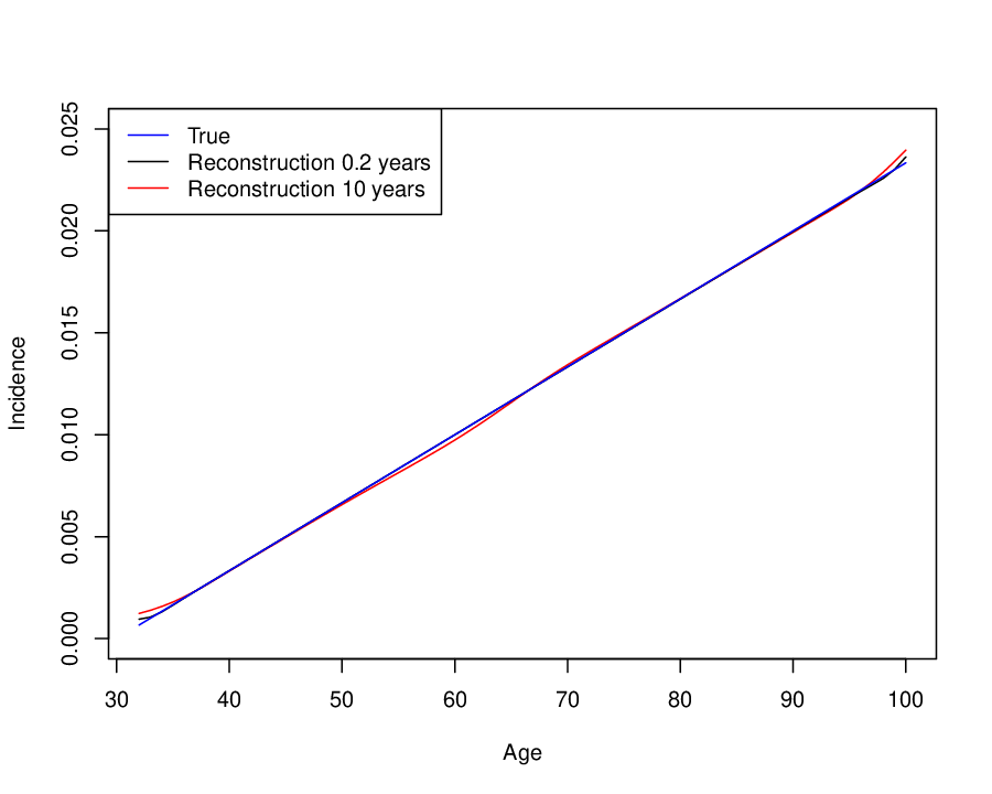
If we use Equation (4) with the approximations (5) and (6) we obtain the reconstructed incidence as shown in Figure 3. The blue line represents the true incidence, the red line the reconstructed incidence. We can see slight differences between these lines. The relative differences (in %) between the reconstructed and the true incidence is shown in Table 1. We can see that the greatest relative deviation occurs at the lowest (7.68% at age 35) and the highest age class (2.66% at age 100). Since these deviations are not attributable to sampling error but just to the approximations (5) and (6) and thus by the choice of $t_{1}$ and $t_{2},$ we call these errors by study design. These errors are intrinsic to the choice of $t_{k},~k=1,2,$ which in an epidemiological application are given by the available data.

We can see that indeed the study design is responsible for the relatively high deviations. If we choose $t_{1}=104.9$ and $t_{2}=105.1,$ we can see that the deviation between the true and the reconstructed incidence decreases. The reconstructed incidence for $\Delta=0.2$ is depicted as a black line in Figure 3. It is closer to the true incidence than the red line. The relative error for this case is shown in the third column of Table 1.

Age	Rel. error (%)	Rel. error (%)
(in years)	$\Delta=10$	$\Delta=0.2$
35.0	7.68	-1.48
40.0	-0.56	0.01
45.0	-0.75	-0.00
50.0	-1.38	0.01
55.0	-2.36	0.01
60.0	-2.61	-0.02
65.0	-0.70	0.00
70.0	0.72	0.01
75.0	0.43	-0.00
80.0	0.06	0.00
85.0	-0.20	-0.00
90.0	-0.39	0.01
95.0	-0.42	-0.00
100.0	2.66	1.54

Table 1: Relative errors of the reconstructed incidences at specific ages. The second and third column shows the relative errors for the inital setting with

\Delta=10

and the decreased relative errors for

\Delta=0.2.

It is important to remember that the deviations described so far are just caused by the choice of the study design, not by any sampling uncertainty. Since we use the approximations in Equations (5) and (6), which are exact only in special cases, we will almost always have an error in the reconstructed incidence.

3.2 Sampling error of the prevalence

In the previous section we have used exact values for $p(t_{k},\cdot),~k=1,2.$ Surveying prevalence in real cross-sectional studies usually suffer from several sources of errors. Examples are measurement errors (i.e., errors in determining the state a subject belongs to in the illness-death model), non-representativeness of the study participants (selection bias), discretisation error and sampling error. We confine ourselves to the last types of errors.

3.2.1 Error types

By discretisation error we mean everything that is related to making the continuous functions $a\mapsto p(t_{k},a),~k=1,2,$ discrete. Typically the prevalence $p(t_{k},\cdot)$ is estimated using finitely many age groups. Assumed we want to estimate $p(t_{k},\cdot)$ at ages $a_{\ell},~\ell=1,\dots,L,$ then all persons alive at $t_{k}$ whose age is in the age group $(a_{\ell}-\varepsilon,a_{\ell}+\varepsilon],~\varepsilon>0,$ are examined if the have the disease or not. Following approximation is used:

p(t_{k},a_{\ell})\approx\frac{\#\text{persons alive at }t_{k}\text{ having the disease and age in }(a_{\ell}-\varepsilon,a_{\ell}+\varepsilon]}{\#\text{persons alive at }t_{k}\text{ with age in }(a_{\ell}-\varepsilon,a_{\ell}+\varepsilon]}.

Situations are easily imaginable, where this estimation is biased, for instance, if $a_{\ell}$ is a local extremum of $p(t_{k},\cdot).$

Finally, by sampling error we mean any effect that is related to having only a sample of the whole population in the study.

3.2.2 Sampling error

To examine the effect of the sampling error, we simulate a population in the illness-death model. Each individual is disease-free at birth and is followed from birth to death (without loss). In each of 70 consecutive years $t=1,\dots,70,$ we consider 300000 persons born with date of birth uniformly distributed across the year. In total 21 million ( $=70\times 300000$ ) persons are simulated. Incidence $i$ and $m_{0}$ are treated as competing risk, and details of the implementation (with source code) are described in (Brinks et al., 2014).

The cross-sections in the years $t_{1}=100$ and $t_{2}=110$ comprise more than 11 million persons alive aged between 40 and 95. The age distribution of the living and the prevalent persons are shown in Table 2.

Age	Cross-section at
group	$t_{1}=100$		$t_{2}=110$
(years)	alive (N)	prevalent (n)	alive (N)	prevalent (n)
(40,45]	1479755	38605	1480777	38391
(45,50]	1467357	72794	1468037	73006
(50,55]	1445529	115689	1445263	115545
(55,60]	1405534	159514	1407035	159795
(60,65]	1333192	194120	1336987	194515
(65,70]	1215229	205780	1218949	206676
(70,75]	1041215	190407	1046718	192903
(75,80]	819662	155683	828053	157549
(80,85]	568871	108209	577779	110667
(85,90]	326252	60093	332622	61667
(90,95]	137577	24146	143004	25145
(40, 95]	11240173	1325040	11285224	1335859

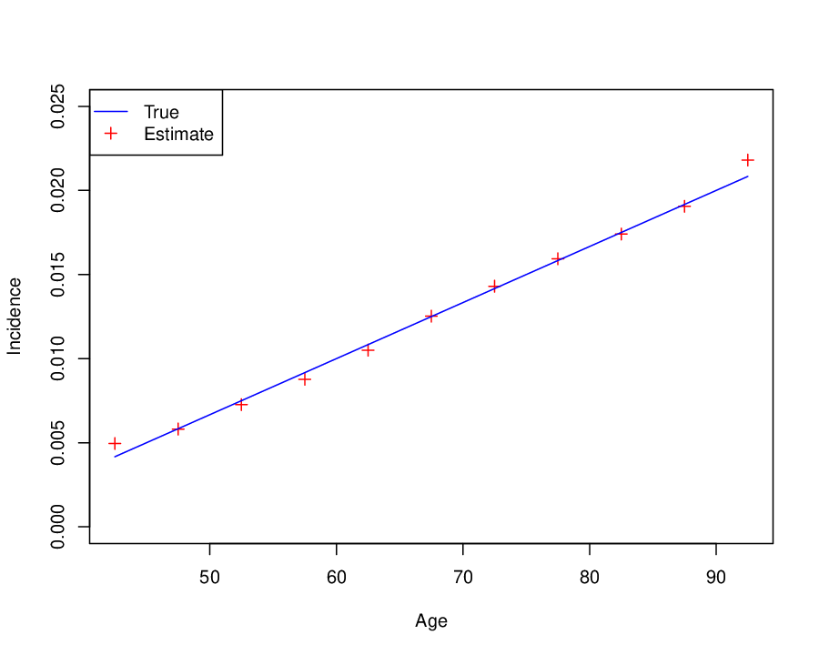
Table 2: Age-distributions of living and prevalent persons in the two cross-sections.

From the resulting age-specific prevalence via Equation (4) with the approximations (5) and (6) we obtain the estimated age-specific incidence $i(t_{s},a_{\ell}),~\ell=1,\dots,L,$ as shown in Figure 4. The error due to the study design is still visible (cf. Figure 3). Table 3 shows the relative errors of the estimated age-specific incidence.

$a_{\ell}$	Rel. error (%)
42.5	18.89
47.5	-0.35
52.5	-3.14
57.5	-4.33
62.5	-3.03
67.5	0.18
72.5	0.97
77.5	0.65
82.5	-0.53
87.5	-0.59
92.5	4.67

Table 3: Relative errors of the estimated age-specific incidence based on the data in Table 2. The numerical values of the estimated incidence are shown in the fourth column of Table 4.

In the next step, we want to study the impact of including a lower number of persons in the cross-sectional studies at $t_{1}$ and $t_{2}.$ For this, we repetitively ( $n_{\text{rep}}=1000$ ) draw samples of different sizes ( $N_{\kappa}$ ) from the population of the 21 million, estimate the incidence for $a_{\ell}$ in the described way and examine the distribution of the $n_{\text{rep}}$ estimates of the incidence.

Figure 5 shows the quantile-quantile plots (Q-Q-plots) of the $n_{\text{rep}}$ repeated estimates for a subpopulation of size $N_{1}=2.6$ million for the different age groups $a_{\ell}$ compared to the normal distribution. In all age groups $a_{\ell}$ the Q-Q-plots indicate that the estimates are normally distributed. For $N_{\kappa},~\kappa=2,3,$ these Q-Q-plots (not shown here) allow the same conclusion.

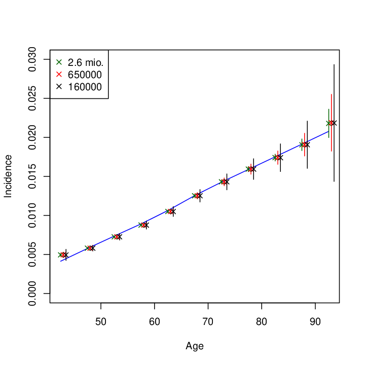
Based on the observation that the incidence estimates follow a normal distribution (see Figure 5), the distribution may be characterised by mean and standard deviation (SD). The fifth to the tenth column of Table 4 show the corresponding values for $N_{1}=2.6$ million, $N_{2}=650000$ and $N_{3}=130000.$ We can see that the mean of the distribution remains stable whereas the SD approximately doubles in each step from left to right. The doubling of the SD is not surprising as $\tfrac{N_{\kappa}}{N_{\kappa+1}}\approx 4,~\kappa=1,2.$

Age	True	Without	Population	$N_{1}=2.6$ mio		$N_{2}=650000$		$N_{3}=130000$
$a_{\ell}$	incidence	sampling	of 21 mio.	Mean	SD	Mean	SD	Mean	SD
42.5	41.7	41.4	49.5	49.9	0.9	49.9	1.8	49.9	3.5
47.5	58.3	57.7	58.1	58.8	0.4	58.8	0.9	58.9	1.9
52.5	75.0	73.6	72.6	72.8	0.5	72.8	1.0	72.6	2.0
57.5	91.7	89.2	87.7	86.5	0.6	86.5	1.3	86.3	2.6
62.5	108.3	106.3	105.1	102.4	0.8	102.3	1.6	102.5	3.3
67.5	125.0	125.4	125.2	120.5	1.0	120.5	2.1	120.6	4.2
72.5	141.7	142.7	143.0	138.1	1.3	138.1	2.5	137.9	5.1
77.5	158.3	158.9	159.4	152.5	1.7	152.4	3.3	152.2	6.6
82.5	175.0	175.1	174.1	168.3	2.1	168.2	4.4	168.0	8.9
87.5	191.7	191.4	190.5	184.4	3.8	184.6	7.7	184.4	15.4
92.5	208.3	207.7	218.1	219.8	9.3	220.0	18.7	221.7	37.9

Table 4: True and estimated incidences in the different age groups based on different prevalence data.

In Figure 6 the mean and the 95% coverage intervals of the estimated incidences based on the different $N_{\kappa},~\kappa=1,2,3,$ are shown. The design error is still visible in the point estimates (cf. Figure 3).

4 Discussion

In this work we examine different sources of errors in a recently proposed algorithm of estimating incidences from two cross-sections. The first source of error is due to the study design. Two cross-sections at different points in time $t_{k},~k=1,2,$ can only approximate the partial derivative of the prevalence. This error is intrinsic of the data sources available. In our example, a smaller difference between the $t_{k}$ is favourable over a larger difference (Table 1). In practice, this may not always be the case. The second source of error, the discretisation error, is a result from estimating the prevalence at a specific age by the prevalence in an age group. Situations are possible, where the prevalence at a specific age is not accurately estimated by the prevalence in an age group. Finally, sampling error due to the limited persons in the cross-sectional studies is examined. It can be seen that imprecise estimates of the prevalence due to few persons in the age groups leads to inaccurate estimates of the incidence.

This work just examines the impact of errors in the prevalence due to study design, discretisation and sampling. In epidemiological applications the estimates of the mortality rates are also subject to errors. These are not considered here. However, this work sketches an easy way to obtain error bounds of incidence estimates in this context as well: Based on the uncertainties in the input values, prevalence and mortality rates, one may draw random samples from the distributions of input values, apply the framework shown in this article and then examine the distributions of the estimated incidences.

References

Brinks et al. (2013) Brinks R, Landwehr S, Icks A, Giani G (2013) Deriving age-specific incidence from prevalence data. Stat Medic 32(12):2070-8 doi:10.1002/sim.5651
Brinks (2013a) Brinks R (2013a) Partial differential equation about the prevalence of a chronic disease in the presence of duration dependency. ArXiv-Preprint http://arxiv.org/abs/1308.6367
Brinks (2013b) Brinks R (2013b) Surveillance of the Incidence of Noncommunicable Diseases (NCDs) with Prevalence Data: Theory and Application to Diabetes in Denmark. ArXiv-Preprint http://arxiv.org/abs/1303.1442
Brinks & Landwehr (2014) Brinks R, Landwehr S (2014) Age- and time-dependent model of the prevalence of non-communicable diseases and application to dementia in Germany. Theor Popul Biol 92:62-8 doi:10.1016/j.tpb.2013.11.006
Brinks et al. (2014) Brinks R, Landwehr S, Fischer-Betz R, Schneider M, Giani G (2014) Lexis diagram and illness-death model: simulating populations in chronic disease epidemiology. PLoS One 12;9(9) doi:10.1371/journal.pone.0106043
Dahlquist & Björck (1974) Dahlquist G, Björck A (1974) Numerical Methods. Prentice Hall, New Jersey
Kalbfleisch & Prentice (2012) Kalbfleisch JD, Prentice RL (2002) The Statistical Analysis of Failure Time Data, 2nd edn. John Wiley & Sons, Hoboken, NJ
Keiding (1991) Keiding N (1991) Age-specific incidence and prevalence: a statistical perspective. J R Statist Soc A 154:371-412