Nonminimal Higgs Models, Dark Matter, and Evolution of the Universe^a

Nonminimal models of electroweak symmetry breaking – models with additional Higgs bosons – are discussed in this work with the focus on difficulties and possibilities of the experimental observation of new particles predicted in such theories taking into account recent data on the properties of the Higgs boson obtained at the LHC (Sections 2-5). A special variant of a Two Higgs Doublet Model– the inert doublet model (IDM)-naturally introduces candidates for dark matter particles. A method for the measurement of the masses of these particles at the ILC linear collider has been discussed. It is found that strongly interacting dark matter can exist within this model (Sections 6 and 7). The parameters of the potential of the IDM vary in the process of cooling of the Universe in the postinflation era and the phase states of the Universe can change so that, after the usually discussed phase transition breaking electroweak symmetry, the Universe can undergo an additional first order phase transition or a pair of second order phase transitions at fairly low temperatures with a rich structure of critical fluctuations (Sections 8 and 9).

The electroweak theory describes experimental data well. To complete the development of the theory, it remained to reveal how electroweak symmetry breaking (EWSB) occurs. After the detection of the Higgs boson with the mass $M_{h}=125$ GeV [1], the physics community believes that EWSB is due to the Higgs mechanism with the Lagrangian

Here ${\cal L}^{SM}_{gf}$ describes the standard $SU(2)\times U(1)$ interaction of the gauge bosons and fermions, ${\cal L}_{Y}$ is the Yukawa interaction of fermions with scalar Higgs fields $\phi_{i}$, and the last two terms describe the Higgs fields ($T=\sum_{i}({\cal D}_{\mu}\phi_{i})({\cal D}_{\mu}\phi_{i})^{\dagger}/2$ is the standard kinetic term and $V$ is the Higgs potential).

The minimal variant (Standard Model) includes one fundamental Higgs field $\phi$ (weak isodoublet) and $V=-m^{2}(\phi^{\dagger}\phi)/2+\lambda(\phi^{\dagger}\phi)^{2}/2$. The field $\phi$ has four degrees of freedom. After EWSB, three components of this field remain massless. These are Goldstone modes, which become the longitudinal components of gauge fields. One component is manifested as a scalar Higgs boson whose mass is an almost arbitrary parameter of the theory. The coupling constants of the Higgs boson with fundamental particles are unambiguously determined.

The same EWSB mechanism can also be implemented in nonminimal models containing several fundamental Higgs fields $\phi_{i}$. They allows the natural description of the CP symmetry breaking and flavor changing neutral currents, as well as the introduction of candidates for dark matter particles, etc. (Such models naturally appear in, e.g., models of broken supersymmetry for the description of reality: MSSM, nMSSM, etc.). Models nHDM + pHSnM containing n scalar isodoublets and p scalar isosinglets will be specially considered below. (The Higgs sectors in MSSM and nMSSM have the form 2HDM and 2HDM + 1HSnM, respectively.)

$\bullet$ The relative coupling constants of gauge bosons $V=Wm\,Z$, leptons and quarks $f$ with the neutral Higgs boson $h_{a}$ are the ratios of the observed constant values to the respective values in the Standard Model (SM):

The nonminimal Higgs models include additional interactions of scalar and vector bosons. In models with one charged Higgs boson $H^{\pm}$, the quantities

are introduced.

$\bullet$ SM-like situation. After EWSB, new fundamental fields appear in the form of a set of charged and neutral scalar Higgs bosons H± and ha. The observation of these new bosons will be the main indication of the realization of nonminimal models. The deviation of the coupling constant values from their values in the Standard Model will be a preliminary signal of the realization of such a model.

In view of this circumstance, the following question arises. Let the experimental situation at a certain time be indistinguishable within the experimental accuracy from that predicted by the Standard Model; i.e., only one Higgs boson is detected and its interactions with fundamental particles within the experimental accuracy ${\varepsilon}^{exp}$ do not differ from the predictions of the Standard Model:

This situation is called by us the SM-like situation [2]. Is this compatible with the realization of some nonminimal theory? What are the ”simplest” experiments that make it possible to distinguish these possibilities?

The SM-like situation in the nonminimal model can occur if additional Higgs bosons are very heavy and are coupled only weakly with usual matter (decoupling limit). In [2] it was found that, at the experimental accuracy expected at the LHC, which was being built at that time, and at the planned linear $e^{+}e^{-}$ collider, even the simplest nonminimal model 2HDM with the special choice of the Yukawa interaction 2HDM-II (as in MSSM) allows several possibility windows significantly differing from the decoupling limit and implementing the SM-like situation. It is clear that such windows exist in other models as well. (At the same time, study of the production of the Higgs boson at a photon collider will promote the choice between the models [2].)

Successful experiments (decrease in ${\varepsilon}^{exp}$) reduce the region of the allowed parameters of nonminimal model (3).

The LHC experiments indicate the realization of the SM-like situation [1], [3] (with inaccuracies much larger than those discussed in [2]). The world physics community is now actively seeking such possibilities and probable signals of deviations from the Standard Model in future experiments.

The simplest alternative to the minimal variant of the Standard Model is the model with two Higgs doublets $\phi_{1}$ and $\phi_{2}$ (2HDM). Its potential is generally described by 14 parameters (4 complex parameters $m_{12}^{2}$ and $\lambda_{5-7}$ and real valued remaining parameters):

Different variants of the model differ in the form of the Yukawa interaction ${\cal L}_{Y}$.

Owing to the presence of two fields with identical quantum numbers in the model, the same physical reality can be described by different forms of the Lagrangian. They can be transformed to each other by a global linear transformation of the fundamental Higgs fields (generalized rotation$\phi_{1},\phi_{2}\to\phi_{1}^{\prime},\phi_{2}^{\prime}$) with the appropriate variation of the parameters of the potential (reparameterization (RPa) invariance). The mentioned rotation is described by three (gauge) parameters. Consequently, it is sufficient to determine 11 significant parameters for the complete description of the model.

The potential has a minimum at certain values $\langle\phi_{i}\rangle$ of classical fields. The isotopic direction corresponding to the neutral field along the lower component of the weak isospinor $\langle\phi_{i}\rangle$ is usually chosen. Correspondingly, the minimum conserving the charge has the form

Under RPa rotation, the ratio $v_{2}/v-1=\tan\beta$ varies and $v=\sqrt{v_{1}^{2}+v_{2}^{2}}=246$ GeV is conserved.

Different RPa gauges are convenient for solving different physical problems. In particular, for studying consequences of some symmetry, it is preferable to use a gauge in which this symmetry is written in the simplest form.

The Higgs basis in which $\langle\phi_{1}\rangle=\dfrac{1}{\sqrt{2}}\begin{pmatrix}0\\ v\end{pmatrix}$, and $\langle\phi_{2}\rangle=0$ is convenient in a number of problems (see, e.g. [4]). This basis is obtained from the basis in which v.e.v.’s have the form of Eqs. (5) by the transformation

with the appropriate change in the parameters of the potential $\lambda_{i}\to\Lambda_{i}$ (below, the subscript $H$ will be omitted).

The potential can be represented in the form including the mass of the charged Higgs boson $M_{\pm}$ :

This potential holds its form under the rephasing (RPh) transformation $(\!\phi_{1}^{\dagger}\phi_{2}\!)\to(\!\phi_{1}^{\dagger}\phi_{2}\!)e^{i\rho}$ (6) with the appropriate change in the parameters $\Lambda_{i}$.

Then, the fields are expanded in terms of deviations from the vacuum average:

Here, $G^{\pm}$ and $G^{0}$ are the Goldstone fields transformed to the longitudinal components of massive gauge fields $W^{\pm}$ and $Z$ (they are omitted below), $H^{\pm}$ are the charged Higgs fields with the mass $M_{\pm}$, and neutral Higgs fields $h_{a}$ are formed from neutral components $\eta_{i}$:

The elements of the mixing matrix $R_{a}^{i}$ are real valued. A similar relation can certainly be written in any RPa basis. The advantage (for analysis) of the Higgs basis is that the measurable physical quantities, coupling constants (2) are directly expressed in terms of $R_{a}^{i}$:

(The phases of the quantities $\chi^{(a)}_{H^{\pm}W^{\mp}}$, i.e., the ratios $R_{a}^{3}/R_{a}^{2}$, cannot be fixed because of the presence of phase freedom in the definition of fields in Eq. (7), but their relative phases are unambiguously defined. In particular, the gauge of this phase can be fixed by the requirement that one of the parameters $\chi^{(a)}_{H^{\pm}W^{\mp}}$ be real valued.)

The direct consideration of Eq. (7) makes it possible to verify that the parameters of the model are classified into two groups. The parameters in the first group ($\Lambda_{1},\,\Lambda_{4},\,\Lambda_{5},,\Lambda_{6}$, $M^{2}_{\pm}$, $v^{2}$) are completely determined by the masses of scalar particles and their coupling constants with gauge bosons. The remaining parameters ($\Lambda_{3},\,\Lambda_{7},\,\Lambda_{2}$) cannot be determined without the measurement of triple and quadruple interactions of Higgs bosons (the $H^{+}H^{-}h_{a}$ and $H^{+}H^{-}H^{+}H^{-}$ vertices are the best candidates for these interactions). Furthermore, even at moderate masses of Higgs bosons, a scenario with large $\Lambda_{2}$ values is possible (strong interaction in the Higgs sector, which should be studied separately [6]). This is the difference from the Standard Model, where the physical Higgs boson disappears under the strong coupling conditions and the width of the Higgs boson becomes comparable to its mass.

The orthogonality of the mixing matrix means that $\sum\limits_{i}|R^{a}_{i}|^{2}=1$ and $\sum\limits_{a}|R^{a}_{i}|^{2}=1$. These relations together with (10) can be represented in the form of the sum rules [6]

The presented method of obtaining sum rules makes it possible to expand these rules to much wider classes of models.

$\bullet$ Sum rule (11a) is well known in 2HDM [7, 2, 8] and means that the masses of gauge bosons are determined by the Higgs mechanism of EWSB. For this reason, sum rule (11a) is valid in any nonminimal Higgs model both such that $\chi_{W}^{(a)}=\chi_{Z}^{(a)}$ (as in the Standard Model and nHDM) and such that $\chi_{W}^{(a)}\neq\chi_{Z}^{(a)}$ (e.g., models with additional isosinglet and (or) isotriplet Higgs fields) [9].

Sum rules (11b) and relation (11c) are formulated for the first time. They are valid for all models whose physical sector includes only one charged Higgs boson ($H^{\pm}$). These are models including two isodoublets and p isosinglets, 2HDM + pHSnM, in particular, nMSSM.

Sum rules (11a)-(11c) describe the Higgs sector of theory at any type of (Yukawa) interaction with fermions. Sum rules are known for (generally complex) coupling constants of a certain fermion (quark or lepton) $f$ with neutral Higgs bosons $\chi_{f}^{(a)}$ in models with two Higgs doublets and a certain type of their interaction with fermions, 2HDM-II and 2HDM-I [7, 2, 8]:

$\bullet$ We found that these sum rules are extended for the nHDM + pHSnM models with arbitrary n and p values if weak isoscalar fields are not coupled to fermions and without additional limitations for the form of the Yukawa interaction [9]. To prove this statement, let us write the general interaction of the fermion $f$ with the fundamental Higgs isodoublet in the form $\Delta L_{Y}=\sum_{j}g_{jf}\bar{\psi}^{\dagger}\phi_{j}\psi_{f}$. The simple reparameterization $\phi_{1}^{\prime}=N\sum_{j}g_{jf}\phi_{j}$ (where $N$ is the normalization factor) transforms this contribution to the form $\Delta L_{Y}=g_{1f}^{\prime}\bar{\psi}^{\dagger}\phi_{1}^{\prime}\psi_{f}$, which coincides with the form of the corresponding interaction in 2HDM-II (or 2HDM-I), where sum rule (12) has already been proven.

Relations between Yukawa constants for different fermions appear only under special assumptions on the structure of this interaction.

$\bullet$ On the strategy of search for new Higgs bosons at colliders in the SM-like situation.

The main problem of the verification of nonminimal models is search for new neutral Higgs bosons $h_{a}$ with masses $M_{a}$ and widths $\Gamma_{a}$ (we consider new Higgs bosons different from the already detected one, $a\neq 1$, and having masses $M_{a}>150$ GeV). In various particular models, such problems have been discussed for many years, as a rule, for certain masses of these particles. Until recently, it was commonly expected that the properties of this boson $h_{a}$ are close to those of the would be standard Higgs boson in the Standard Model with approximately the same mass. In view of the SM-like situation, these expectations are unjustified in any nonminimal model.

Decay channels and widths $\Gamma_{a}$ a of Higgs bosons $h_{a}$. In the Standard Model, the main contribution to the width of the Higgs boson with masses larger than 150 GeV comes from the decays $h\to W^{+}W^{-}$ and $h\to ZZ$. These decays would give the main signal of the detection of the CP even Higgs boson. According to sum rule (11a), the coupling constants of new Higgs bosons $h_{a}$ are small. Therefore, the detection of bosons $h_{a}$ through their decays into gauge bosons is highly improbable (while detection through decays into quarks is difficult because of a large background). For the same reason, the widths $\Gamma_{a}$ at $Ma<350$ GeV are very small in any nonminimal Higgs model. In this case, the main decay channel is again $h_{a}\to\bar{b}b$ with very large background; consequently, the detection of each $h_{a}$ is a difficult problem.

At $Ma>350$ GeV, the $h_{a}\to\bar{t}t$ decay channel is open. Sum rule (12) includes the coupling constants $\chi_{t}^{(a)}$, which are generally complex. The smallness of the sum $\sum\limits_{a>1}(\chi_{t}^{(a)})^{2}=1-(\chi_{t}^{(1)})^{2}$ can be ensured at large individual terms (e.g., one is real and the other is imaginary). Such an example occurs in 2HDM-II at $\tan\beta<1$ (values $\tan\beta<1/7$ should be excluded because this is the region of strong Yukawa interaction, where perturbative estimates are invalid). In this case, the ratios $\Gamma_{a}/M_{a}$ at least for a pair of bosons $h_{a}$ can be non small and be approximately equal to each other [9]. At $\tan\beta\gtrsim 1$, the total width $\Gamma_{a}$ is small at any mass $M_{a}$.

Production of the CP even Higgs boson through a gauge vertex was until recently assumed to ensure the best signal/background ratio and the least inaccuracy in the measurement of its parameters: $W$ fusion at the LHC, $e^{+}e^{-}\to Zh_{a}$ and $e^{+}e^{-}\to\nu\bar{\nu}h_{a}$ at the ILC, and $e\gamma\to\nu W^{-}h_{a}$, $\gamma\gamma\to W^{+}H^{-}h_{a}$ at the PLC (photon collider).

In view of Eq. (3), it follows from sum rules (11a) for all models with any set of their parameters that experiments on the search for additional Higgs bosons at the LHC and linear collider in such processes cannot be successful [9] (such results were obtained till now only at some sets of parameters in separate models (see, e.g., recent works [10]).

Processes of production of the Higgs boson together with the $t$ quark and through the loop vertex at the LHC ($gg\to t\bar{t}h_{a}$, $gg\to h_{a}$) and at photon collider ($\gamma\gamma\to h_{a}$, $e\gamma\to eh_{a}$) require a separate discussion.

$\bullet$ Sum rules (11b) and relations (11) show that search for Higgs bosons $h_{a}$ can be successful in the $q_{1}\bar{q}_{2}\to H^{+}h_{a}$, $q\bar{q}\to h_{a}h_{b}$ at LHC, $e\gamma\to\nu H^{+}h_{a}$, $e^{+}e^{-}\to h_{a}h_{b}$, $e^{+}e^{-}\to H^{\pm}W^{\mp}h_{a}$ at ILC, $\gamma\gamma\to H^{\pm}W^{\mp}h_{a}$ at PLC.

By construction, most of the nonminimal models are symmetric under a certain group of global transformations, which can concern both the scalar and fermion sectors of a model. Spontaneous symmetry breaking can be responsible for candidates to dark matter particles, CP violation, etc.

Despite importance of symmetries and numerous phenomenological studies, it was unknown till now what symmetry groups can appear in such models, how these symmetries can be broken, how they are manifested in the scalar and fermion sectors, and what their phenomenological consequences are. Only the simplest variants have been analyzed.

Most of the arising problems in a very wide class of models were solved in [11]-[21], where new results were obtained and new methods for analyzing these models were developed. These methods are often much more efficient than traditional approaches and sometimes reveal some imperfections of these approaches.

A. The problem of classification of symmetry groups within the scalar sector was studied for theories with a given set of additional scalar fields. This problem was previously solved only for 2HDM. The Abelian part of this problem was solved for a model with arbitrary number of doublets [12]. This problem was completely solved for 3HDM [14, 16]. In the process of solution, a method for analysis of Abelian symmetries was developed on the basis of normal Schmidt forms, which is appropriate for any models with new complex fields.

A class of always broken symmetries called frustrated was described [11]. A new geometric method of the minimization of potentials with such symmetries was proposed [17]. This method is sometimes better than more standard methods.

Geometric CP breaking in multidoublet models was analyzed [20].

B. Scalar candidates to dark matter particles with unusual quantum numbers naturally appear in multidoublet models [13]. A new convenient criterion that cuts off models with metastable vacuum was found for the two doublet model [18, 19]. This criterion can be verified using LHC data.

C. The problem of classification of symmetries and study of their consequences was considered in the quark sector of multidoublet models [21]. The general results concerning possible symmetries for an arbitrary number of doublets were obtained. The most interesting examples of 3HDM and 4HDM were analyzed. The method used leads to results without computer calculations, opening a direct way to neutrino models.

The inert doublet model is a serious candidate to the description of dark matter [22]. This model is described by a special variant of 2HDM, where one Higgs field $\phi_{S}$ is the same as in the minimal Standard Model and the other Higgs field $\phi_{D}$ does not have a vacuum average and does not interact with fermions. The corresponding Lagrangian is given by eqs. (1), (4) with $\phi_{1}\to\phi_{S}$, $\phi_{2}\to\phi_{D}$, $m_{12}=0$, $\lambda_{6}=\lambda_{7}=0$.

The parameter $\lambda_{5}$ can be taken real and negative. In addition, we assume $\lambda_{4}+\lambda_{5}<0$.

Below, the following notation will be used:

The requirement of the positive potential at large semiclassical fields imposes the constraints $\lambda_{1},\lambda_{2}>0$ and $R>-1$.

The potential has a pair of $Z_{2}$ symmetries (under the transformation $\phi_{S}\to-\phi_{S}$, $\phi_{D}\to\phi_{D}$), which is called $S$ symmetry and $D$ symmetry (under the transformation $\phi_{S}\to\phi_{S}$, $\phi_{D}\to-\phi_{D}$). The Yukawa interaction breaks $S$ symmetry, whereas $D$ symmetry is exact, ensuring conservation of the $D$ parity under this transformation. The model can pretend to describe dark matter with the set of parameters such that $\langle\phi_{D}\rangle=0$ and $\langle\phi_{S}\rangle=v/\sqrt{2}$. At this minimum of the potential, $D$ symmetry remains exact and $S$ symmetry is broken by the Yukawa interaction and by the choice of the minimum of the potential. The masses of fermions are expressed in terms of $\langle\phi_{S}\rangle$ as in the Standard Model. To implement this state and a neutral particle for dark matter, the parameters of the potential should satisfy the conditions

Expansion (8) now becomes

Here, $h$ is the standard Higgs boson with the mass $M_{h}=125$ GeV; $D$, $D_{A}$, and $D^{\pm}$ are physical particles with the masses $M_{D}$, $M_{A}$, $M_{\pm}\equiv M_{+}$, respectively;

The $P$ parities of $D$ and $D_{A}$ are opposite to each other.

Particles $D$, $D_{A}$ and $D^{\pm}$ are $D$ odd. All other particles are $D$ even. In view of the conservation of the $D$ parity, the lightest of $D$ particles, $D$, can serve as dark matter.

The masses of $D$ particles are limited by the accelerator and cosmological data [23, 24]. In particular, $M_{+}>90$ GeV and $M_{A}+M_{D}>180$ GeV (LEP data).

The scalar particles $D,\,D_{A}$, and $D^{\pm}$ interact with usual particles through covariant derivatives in the kinetic term $({\cal D}_{\mu}\phi_{D})^{\dagger}({\cal D}_{\mu}\phi_{D})$.. Triple interactions with gauge bosons have the form $D^{+}D^{-}\gamma(Z)$, $D^{\pm}DW^{\mp}$, $D^{\pm}D_{A}W^{\mp}$, $DD_{A}Z$. Interactions with the Higgs boson $h$ are diagonal in each of the fields $D$, $D_{A}$ and $D^{\pm}$. To describe them, the constant $\lambda_{3}$ should be added to the constants obtained from the measured masses of the particles. At $M_{D}<60$ GeV, measurements of the invisible decay $h\to DD$, e.g., in the $e^{+}e^{-}\to Zh\to ZDD$ reaction will allow determination of $\lambda_{3}$.

$\bullet$ Strongly interacting dark matter [25]. The complete set of quadratic interactions between $D$ particles has the form

Differences of the masses of $D$ particles are independent on $\lambda_{2}$. Their coupling constants to gauge bosons and to the standard Higgs boson $h$ are independent on $\lambda_{2}$. Thus, large $\lambda_{2}$ values corresponding to strongly interacting dark matter are not excluded. This interaction at low energies of colliding $D$ particles is repulsion ($\lambda_{2}>0$). At high energies, attraction can appear with the formation of resonance states, as was discussed for possible strong interaction in the Higgs sector of the Standard Model (see, in particular, recent work [26]). In this case, further studies are necessary.

The $D^{+}D^{-}$ pair is produced at the ILC linear collider with the appropriate energy in $e^{+}e^{-}$ collisions with the cross section close to the cross section for the $e^{+}e^{-}\mu^{+}\mu^{-}$ process. These cross sections are very large for the ILC. Pairs of hadronic jets will be observed (hadronic decay modes of W), as well as leptons from the $D^{+}\to DW^{+}$ decay. The total energy of the observed particles is much lower than the total energy of the collision and their total transverse momentum is quite high. If the energies of hadronic jets produced from the decay of W could be accurately measured, the measurement of the boundaries of the corresponding energy distributions would make it possible to determine the masses of $D^{+}$ and $D$. Unfortunately, such accurate measurements are impossible. Only the energies of leptons (e.g., muons) from the decay of $W$ can be measured well. Simple kinematic analysis shows that the energy distributions of muons have reliably determined singularities (peaks and kinks), measurement of which will allow accurate determination of the masses of $D^{+}$ and $D$ [27].

This kinematic analysis is independent of the spin of $D$ particles and can be applied in the case of fermion dark matter (e.g., if $D$ is neutralino and $D^{\pm}$ is chargino). In the latter case, the cross section for the $e^{+}e^{-}\to D^{+}D^{-}$ process is at least twice as large as the same cross section for scalar particles. Thus, after the determination of the masses of particles from the kinematic singularities, even rough measurement of the cross section will make it possible to determine the spin of $D$ particles [27]. More detailed calculations for the IDM (but without study of aforementioned singularities of the energy spectra of an individual lepton) were performed in [28].

The ground state of the Universe in the period of cooling after the Big Bang is determined by the minimum of the Gibbs potential

The Gibbs potential for the IDM in the first nontrivial approximation at quite high temperatures has the form of Eq. (4) with the same coefficients $\lambda_{i}$, but with the mass term depending on the temperature:

Here, $g$ and $g^{\prime}$ are the standard gauge coupling constants of the electroweak theory while $g_{t}\approx 1$ and $g_{b}\approx 0.025$ are the coupling constants of the $t$ and $b$ quarks with the Higgs boson¹¹ 1 This is the high-temperature approximation. At moderate energies, dependencies become more complicated. We hope that our calculations correctly describe the general qualitative picture of phenomena.. In view of positivity constraints, $c_{1}+c_{2}>0$ [23].

Conditions (14) can be violated at finite temperatures. In this case, the properties of the ground state can be significantly different from the present properties [29].

All extrema of the IDM potential are easily obtained because it has a simple structure. These extrema are listed below with the corresponding values $v_{i}=\sqrt{2}\langle\phi_{i}\rangle$ and energy of the ground state ${\cal E}$ [23]:

(If one of the quantities $v_{S}^{2}$ and $v_{D}^{2}$ in (20d) is negative, the extremum $\boldsymbol{M}$ does not realized.)

The ground state (vacuum) corresponds to the extremum with the lowest energy $\cal E$. All possible vacuum states (20) are briefly described below.

$\bullet$ EW symmetric state $\boldsymbol{EWs}$. This extremum exists at any parameters of the potential. It conserves the $D$ and $S$ symmetries of the potential, and is a minimum realizing vacuum at

In this vacuum all particles are massless except for scalar doublets with the masses $|m_{11}|/\sqrt{2}$ and $|m_{22}|/\sqrt{2}$.

$\bullet$ Inert state $\boldsymbol{I_{1}}$. The properties of this state are described in Section 6. It is the ground state (vacuum) under conditions (14).

In two other phases described below, there are no particles having the properties of dark matter.

$\bullet$ Inert-like state $\boldsymbol{I_{2}}$. At first glance, the properties of this state are similar to the properties of the inert state with the change $D\leftrightarrow S$. However, $S$ particles in this state that are similar to $D$ particles in the inert state interact with fermions, which remain massless. The conditions of realization of the state I2 as vacuum are similar to conditions (14):

$\bullet$ Mixed state M. In this state, both $D$ and $S$ symmetries are broken. Here, the masses of fermions are expressed via their present values as $m_{f,M}=m_{f}(v_{S}/v)$. The standard expansion near this extremum gives Goldstone bosons $G^{\pm}$, $G^{0}$, charged Higgs bosons $H^{\pm}$, a pseudoscalar particle $A$ with the masses

and two scalar particles $h$ and $H$ with the masses

According to Eq. (20), if the mixed state gives a minimum of the potential, this minimum is global; i.e., it is vacuum. This occurs under the conditions $|R|<1$ and

$\bullet$ Degeneracy of the mixed state [25]. The initial Lagrangian is symmetric under replacement $\phi_{D}\to-\phi_{D}$. Hence, extremum (20d) is degenerate in the sign of $\langle\phi_{D}\rangle\equiv v_{D}$ and there are states $MP+$ with $\langle\phi_{D}\rangle=|v_{D}|$ and $M_{-}$ with $\langle\phi_{D}\rangle=-|v_{D}|$. In these states, the signs of the coupling constants of the heavy Higgs boson $H$ with the gauge boson $Z$ are different. This difference can be detected in the $t\bar{t}\to WW$ process, where the $Z$ and $H$ exchanges interfere.

The height of the energy barrier between the states $M_{+}$ and $M_{-}$ is given by the energy of a saddle point between them, i.e., by the extremum next in magnitude in Eqs. (20). The height of this barrier ${\cal E}_{B}$ is

The possible phase history of the Universe within the IDM will be described below under the assumption that the present state is the inert vacuum I1.

It is convenient to use the phase plane $\left(\mu_{1}(T),\,\mu_{2}(T)\right)$, where

with the functions $m_{ii}^{2}(T)$ defined by Eq. (19) (the argument $T$ is omitted in the present $\mu_{i}$ values). The present state of the Universe is shown in the figures by the black point $Pn=(\mu_{1},\,\mu_{2})$, where $n$ is the number of the point. Now, in the inert phase, $\mu_{1}>0$. The parameter $\mu_{2}$ can be both positive (points $P1$ and $P3$) and negative (points $P2$ and $P4$). At $R>0$, we have $c_{2}>0$ and $c_{1}>0$ [23], and in the initial state of the Universe ($T\to\infty$) we have $m_{11}^{2}<0$ and $m_{22}^{2}<0$; i.e., this initial state has electroweak symmetry.

In accordance with Eq. (19), the evolution of the Universe is described by the ray nm, which ends at the point $Pn$ (m is the number of the type of ray). The arrow in this ray corresponds to an increase in the time (a decrease in the temperature). The directions of the rays are given by the parameters $\tilde{c}_{1}\equiv c_{1}/\sqrt{\lambda_{1}}$ and $\tilde{c}_{2}\equiv c_{2}/\sqrt{\lambda_{2}}$.

$\bullet$ For the case $\boldsymbol{R>1}$, the phase diagram is shown in left plot of Fig. 1. It contains one quadrant with the $EWs$ phase and two sectors with the phases $I_{1}$ and $I_{2}$. These sectors are separated by the phase transition line $\mu_{1}(T)=\mu_{2}(T)$ (thin black line). Two typical possible present day states are represented by the points $P1$ ($\mu_{2}>0$) and $P2$ ($\mu_{2}<0$) while the possible types of evolution are given by the rays 11, 12, and 21.

$\Box$ Rays 11 ($\boldsymbol{c_{2}/c_{1}>m_{22}^{2}/m_{11}^{2}}$) and 21 ($\boldsymbol{m_{22}^{2}<0}$). Evolution starts from the EW symmetric phase $EWs$. As in the Standard Model, the Universe occurs in the present inert phase after the single EWSB second order phase transition at $m_{11}^{2}(T)=0$, i.e., at the temperature

with the order parameter $\eta_{EW1}\propto\langle\phi_{S}\rangle=v_{S}$, which is represented by the mass of the usual Higgs boson $M_{h}$.

$\Box$ Ray 12 ($\boldsymbol{c_{2}/c_{1}<m_{22}^{2}/m_{11}^{2}}$). Evolution starts from the $EWs$ phase. Then, the Universe goes to the inert-like phase $I_{2}$ at $m_{22}^{2}(T)=0$, i.e., at the temperature

That is EWSB phase transition of the second order with the order parameter $\eta_{EW2}\propto\langle\phi_{D}\rangle=v_{D}$, which is represented by the mass of the Higgs boson $M_{hD}$.

Upon the further cooling, the Universe goes into the inert phase $I_{1}$ at $\mu_{2}(T)=\mu_{1}(T)$, i.e., at the temperature

That is a first order phase transition with the latent heat

Near this phase transition, the usual formation of bubbles of a new phase occurs, which is manifested in the present spatial structure of the cosmic microwave background. This transition can occur at much lower temperature than the EWSB phase transition in the Standard Model.

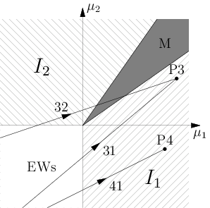
$\bullet$ For the case $\boldsymbol{1>R>0}$, the phase diagram is shown in right plot of Fig. 1. In addition to the phases of the preceding case (left plot), a new (grey in figure) sector with the mixed M phase appears in the upper right quadrant; according to Eq. (25), its boundaries are given by the relations

Two typical possible present day states are shown by the points $P3$ ($\mu_{2}>0$) and $P4$ ($\mu_{2}<0$) and the rays 31, 32, and 41 represent the possible paths of evolution.

$\Box$ Phase evolution for the 31 and 41 rays is similar to that at rays 11 and 21 in left plot.

$\Box$ Ray 32 ($\boldsymbol{c_{2}/c_{1}<m_{22}^{2}/m_{11}^{2}}$). The Universe starts from the $EWs$ state. the Universe goes to the inert-like phase $I_{2}$ at $m_{22}^{2}(T)=0$, i.e., at the temperature $T_{EWs,2}$, given by eq. (29). Just as in the previous case that is EWSB phase transition of the second order with the order parameter $\eta_{EW2}\propto\langle\phi_{D}\rangle=v_{D}$, which is represented by the mass of the Higgs boson $M_{hD}$. With further cooling, the Universe passes through the mixed phase $M$ to the present day inert phase $I_{1}$.

The phase transition $I_{2}\to M_{\pm}$ occurs at the temperature

That is the second order phase transition with the order parameter $\eta_{I2M}\propto\langle\phi_{D}\rangle=v_{D}$, the latter is given by the mass of the ”usual” Higgs boson $M_{hD}$ at in the inert-like phase $I_{2}$ and by the mass of the lightest Higgs boson $M_{h}$ in the mixed phase $M_{\pm}$. The energy barrier between the phases $M_{+}$ and $M_{-}$, given by Eq.  (26) increases as $\eta_{I2M}^{4}$ on departure from the transition point.

When the temperature decreases below $T_{2,1}$ (30), we turn to the region $\mu_{1}>\mu_{2}$ with the change of the order parameter from $\eta_{I2M}$ to $\eta_{MI1}\propto\langle\phi_{S}\rangle=v_{S}$, which is represented by the mass of the modern Higgs boson $M_{h}$ in the inert phase $I_{1}$ and by the mass of the lightest Higgs boson $M_{h}$ in the mixed phase $M_{\pm}$. After that, the energy barrier decreases as $\eta_{MI1}^{4}$. At the temperature

the $M\to I_{1}$ phase transition occurs. That is the second order transition with the order parameter$\eta_{MI1}$.

When approaching the transition temperatures $T_{phtr}=T_{2,M}$ and $T_{M,1}$, the masses of bosons representing the order parameters tend to zero as $M_{a}^{2}=A_{a}|T^{2}-T^{2}_{phtr}|$ with different coefficients $A_{a}$.

Near these transitions, large critical fluctuations appear; their footprints can be sought in the present spatial structure of the cosmic microwave background. In particular, the mixed phase $M$ near $I_{2}\to M$ transitions is built from domains of 3 types, that are $I_{2}$ phase domains (obliged by fluctuations of the temperature and density), and domains $M_{+}$ and $M_{-}$ with the height of walls between domains $\propto\eta_{2,M}^{4}$. The spatial distribution of these domains varies continuously. The characteristic correlation radius of a domain is $R_{c}(T)\propto 1/\eta_{2,M}\propto 1/\sqrt{|T^{2}-T_{2,M}^{2}|}$.

With further cooling, $I_{2}$ domains become less energy preferred, their number is decreased, the $M_{+}$ and $M_{-}$ domains are ”tempered”; i.e., the height of walls between them increases. Domains are transformed to bubbles with the surface tension $\sigma_{s}\sim E_{b}R_{c}$. The curved surface of such bubbles produces pressure $\sim\sigma_{s}/r$, where $r$ is the local radius of curvature. Large domains absorb small domains owing to this pressure. The local velocity of a domain wall is about the speed of light $c$. At the same time, the global mixing process is a slow diffusion process with the characteristic time $\sim(R/c)\sqrt{R/R_{c}}$, where $R$ is the characteristic dimension of the inhomogeneity of the Universe.

When the temperature decreases below $T_{2,1}$, evolution of domains proceeds by the inverse way with the change in the order parameter $\eta_{2,M}\to\eta{M,1}$.

$\bullet$ At $\boldsymbol{0>R>-1}$, the phase diagram is similar to that in right plot of Fig. 1, but with an important change: the region of the mixed phase covers the entire upper right quadrant, expands beyond it, and is located between the rays $\mu_{2}>\mu_{1}/R$ and $\mu_{2}>\mu_{1}R$. Furthermore, the inequality $c_{2}/c_{1}<0$ can be satisfied in this region. In this case electroweak symmetry of the initial state of the Universe is broken and new types of phase evolution appear starting from the initial inert-like phase $I_{2}$ and arriving at the present inert phase $I_{1}$ either through the mixed phase (as the 12 ray) or through the intermediate phase with electroweak symmetry (two second order phase transitions).

$\bullet$ The presented picture leaves many interesting questions for further studies.

Variants with the transition through the mixed phase or with a first order phase transition.

Depending on the parameters of the model, the last phase transition in the Universe can occur at quite low temperature.

What is the relation between the rate of diffusion equalization of fluctuations and the expansion rate of the Universe? Are there scales at which inhomogeneities of the Universe exist at present?

Variant with the transition through the mixed phase.

How long do footprints of ”tempering” of domains hold in the inert phase?

The reviewed studies were supported by the Russian Foundation for Basic Research (project 11-02-00242 and preceding projects), by the Council of the President of the Russian Federation for Support of Leading Scientific Schools project NSh-3802.2012.2), and by the Division of Physical Sciences, Russian Academy of Sciences (program ”Study of the Higgs Boson and Exotic Particles at the LHC”).

References

- [1] The ATLAS Collaboration. Phys. Lett. B 716, 1 (2012) [arXiv:1207.7214 [hep-ex]]; The CMS Collaboration. Phys. Lett. B 716, 30 (2012) [arXiv:1207.7235 [hep-ex]];
- [2]
I. F. Ginzburg, M. Krawczyk, P. Osland.
2nd ECFA/DESY Study 1998-2001 997-1001; hep-ph/9909455;
Nucl. Instrum. Meth. A 472 (2001) 149-154; hep-ph/0101229;
AIP Conf. Proc. Series 578 (2001) 304, IFT-2001-2, 304; hep-ph/0101331;
Proc. SUSY02 Conference 703-706; hep-ph/0211371. - [3] G. Belanger, B. Dumont, U. Ellwanger, J. F. Gunion and S. Kraml, JHEP 1302 (2013) 053 [arXiv:1212.5244 [hep-ph]]
- [4] C. C. Nishi Phys. Rev. D 77 (2008) 055009
- [5] I. F. Ginzburg and K. A. Kanishev, Phys. Rev. D 76 (2007) 095013 [arXiv:0704.3664 [hep-ph]].
- [6] I. F. Ginzburg, K. A. Kanishev. Report at SCALARS2011
- [7] J. F. Gunion, H. E. Haber and J. Wudka, Phys. Rev. D 43, 904 (1991).
- [8] I. F. Ginzburg, M. Krawczyk, Phys. Rev. D 72 (2005) 115013; hep-ph/0408011
- [9] I. F. Ginzburg, M. Krawczyk. ArXiv:[hep-ph] 1310.5881
- [10] H.-Y. Ren, L.-H. Xia, Y.-P. Kuang. arXiv: 1404.6367 [hep-ph]; L. Wang, X.-F. Han arXiv:1404.7437 [hep-ph]
- [11] I. P. Ivanov, V. Keus, Phys. Lett. B 695 (2011) 459-462.
- [12] I. P. Ivanov, V. Keus, E. Vdovin. J.Phys. A 45 (2012) 215201.
- [13] I. P. Ivanov, V. Keus, Phys.Rev. D 86 (2012) 016004.
- [14] I. P. Ivanov, E. Vdovin, Phys. Rev. D 86 (2012) 095030.
- [15] I. P. Ivanov, talk given at Rencontres de Vietnam, Quy Nhon, July 15-21, 2012, arXiv:1211.0647 [hep-ph]
- [16] I. P. Ivanov, E. Vdovin, Eur.Phys.J. C 73 (2013) 2309.
- [17] A. Degee, I. P. Ivanov, V. Keus, JHEP 1302 (2013) 125.
- [18] A. Barroso, P. M. Ferreira, I. P. Ivanov, R. Santos, J. P. Silva, Eur. Phys. J. C 73 (2013) 2537.
- [19] A. Barroso, P. M. Ferreira, I. P. Ivanov, R. Santos, JHEP 1306 (2013) 045.
- [20] I. P. Ivanov, L. Lavoura, Eur.Phys. J. C 73 (2013) 2416.
- [21] I. P. Ivanov, C. C. Nishi, JHEP 1311 (2013) 069.
- [22] N. G. Deshpande and E. Ma, Phys. Rev. D 18 (1978) 2574; R. Barbieri, L. J. Hall and V. S. Rychkov, Phys. Rev. D 74 (2006) 015007 [arXiv:hep-ph/0603188].
- [23] I. F.Ginzburg, K. A. Kanishev, M. Krawczyk, D. Sokolowska. Phys. Rev. D 82, 123533 (2010), hep-ph/1009.4593
- [24] M. Krawczyk and D. Sokołowska, arXiv:0911.2457; 1305.6266 [hep-ph]; M. Krawczyk, D. Soko³owska, B. Swiezewska, arXiv:1304.7757[hep-ph]
- [25] I. F. Ginzburg. Proc. Scalars 2011, 2013
- [26] A. Urbano, arXiv:1310.5733 [hep-ph]
- [27] I.F. Ginzburg. Journ. of Phys: Conference Series, http://iopscience.iop.org/1742-6596, Phys. Part. Nucl. Lett. 9 (2012) 42; Arxiv. hep-ph/1211.2429; Phys. Part. Nucl. 45 (2014) 207; Journ. Mod. Phys. 5 (2014) 1036-1049; P.A. Krachkov. Phys. Part. Nucl. Lett. 9 (2012) 197
- [28] N. D. Christensen T. H. J. Song and Stefanusa arXiv:1404.6258 [hep-ph]
- [29] I. F. Ginzburg, I. P. Ivanov and K. A. Kanishev, Phys. Rev. D 81 (2010) 085031 [arXiv:0911.2383 [hep-ph]].