跳到论文正文
W Papers独立论文阅读器 arXiv:1410.0749 论文正文 计算阅读时间 · 0%
引用这篇论文根据当前论文元数据生成,正式投稿前建议核对。


License: arXiv.org perpetual non-exclusive license
arXiv:1410.0749v1 [math.AP] 03 Oct 2014

A sign-changing Liouville Equation

Alejandro Sarria Address:  Department of Mathematics
University of Colorado at Boulder
Boulder, CO 80309-0395, USA
Email: alejandro.sarria@colorado.edu
and Ralph Saxton Address:  Department of Mathematics
University of New Orleans
New Orleans, LA, 70148, USA
Email: rsaxton@uno.edu
Date: October 1, 2014
Abstract.

We examine periodic solutions to an initial boundary value problem for a Liouville equation with sign-changing weight. A representation formula is derived both for singular and nonsingular boundary data, including data arising from fractional linear maps. In the case of singular boundary data we study the effects the induced singularity has on the interior regularity of solutions. Regularity criteria are also found for a generalized form of the equation.

Key words and phrases: 
Sign changing weight Liouville equation, blow-up, global existence, Schwarzian derivative.
1991 Mathematics Subject Classification
35B44, 35B10, 35B65, 35Q35, 35B40.

1. Introduction

In this article, we study regularity of periodic solutions to the initial boundary value problem

{∂α​tlnu=f(α)u,α∈(0,1),t>0,u(α,0)=u0(α),α∈[0,1],u(0,t)=u(1,t)=g(t),t≥0\begin{cases}\partial_{\alpha t}\ln u=f(\alpha)u,\,\,\,\,\,\,\,\,\,\,\,&\alpha\in(0,1),\,\,\,t>0,\\ u(\alpha,0)=u_{0}(\alpha),\,\,\,\,\,\,\,\,\,\,\,\,&\alpha\in[0,1],\\ u(0,t)=u(1,t)=g(t),\,\,\,\,\,\,\,\,\,\,\,\,\,&t\geq 0\end{cases} (1.1)

for given bounded continuous functions ff and u0>0u_{0}>0 with prescribed boundary data g>0g>0. Moreover, replacing uu on the right-hand side of (1.1)i) by an arbitrary nonnegative function ℱ⁡(u)∈C1​(0,+∞)\mathcal{F}(u)\in C^{1}(0,+\infty) we also establish regularity criteria for the resulting generalization of (1.1). Note that for u>0u>0 to be α\alpha-periodic, integration of (1.1)i) (or of its generalization) over (0,1)(0,1) requires f⁡(α)f(\alpha) to have at least one zero in (0,1)(0,1) and to change sign if it is not identically zero. We will refer to (1.1) as an initial periodic-boundary value problem for the sign-changing Liouville equation.

Two particular versions of Liouville’s equation

□ψ(x,τ)+ϵeψ=0,ϵ=±1,□≡∂τ2−∂x2\square\psi(x,\tau)+\epsilon e^{\psi}=0,\,\,\,\,\,\,\,\,\,\,\,\,\,\,\,\epsilon=\pm 1,\,\,\,\,\,\,\,\,\,\,\,\,\,\,\,\,\,\square\equiv\partial^{2}_{\tau}-\partial^{2}_{x} (1.2)

occur in various applications ranging from plasma physics and field theoretical modeling to fluid dynamics. This has made both versions of (1.2) a frequent topic of investigation. In particular cases, the equation can be interpreted as a model for a self-interacting scalar field in two-dimensional space-time, whose properties have been the subject of extensive study (see for instance [2]-[11]). Equation (1.1)i) is obtained from (1.2) on changing to characteristic coordinates τ=α+t\tau=\alpha+t and x=α−tx=\alpha-t and setting ψ=ln⁡u\psi=\ln u, with f⁡(α)f(\alpha) replacing ϵ\epsilon in the resulting equation. Further, the elliptic Liouville equation

Δlnϕ=−Kϕ2,Δ≡∂2x+∂2y,\Delta\ln\phi=-K\phi^{2},\,\,\,\,\,\,\,\,\,\,\,\,\,\,\,\Delta\equiv\partial^{2}_{x}+\partial^{2}_{y}, (1.3)

appears in the study of two-dimensional steady, incompressible Euler flow with ϕ=eψ\phi=e^{\psi}, for ψ\psi the stream function relating vorticity to the velocity field, ([15], [3]). As in its hyperbolic counterpart, (1.3) reduces to (1.1)i) along curves α=x+i​y\alpha=x+iy and t=x−i​yt=x-iy for f≡−K2f\equiv-\frac{K}{2} and ϕ2=u\phi^{2}=u.

Amongst its many physical applications, (1.1)i) is found in Riemannian geometry. On prescribing the Gaussian curvature K⁡(x,τ)K(x,\tau) for a pseudo-metric d​s2=gi​j​d​xi​d​xj=e2​v​(x,τ)​(d​x2−d​τ2)ds^{2}=g^{ij}dx_{i}dx_{j}=e^{2v(x,\tau)}(dx^{2}-d\tau^{2}) in two-dimensional Minkowski space, the function vv satisfies the relation

K⁡(x,τ)=−e−2​v​(x,τ)​□​v​(x,τ)K(x,\tau)=-e^{-2v(x,\tau)}\square v(x,\tau)

in isothermal coordinates (x,τ)(x,\tau), ([12]). In the case of constant Gaussian curvature, the change to characteristic variables then leads to Liouville’s equation in the form, ([8]),

∂α​tv=K​e2​v.\partial_{\alpha t}v=Ke^{2v}.

In a related setting, the case of sign-changing KK has been studied recently for an elliptic version of the equation, ([13]).

We note that the relevance of (1.1)i) in the field of fluid dynamics is not limited to the hyperbolic and elliptic models (1.2) and (1.3). Indeed, if we restrict ourselves to quantities uu having constant spatial mean, then for a prescribed periodic function ff and initial data u0≡1u_{0}\equiv 1, (1.1)i) appears in the study of classes of semi-bounded solutions to the three-dimensional incompressible Euler equations, ([9, 16, 14]). In this context, ff controls the concavity of the components of the velocity field and uu represents the jacobian of the transformation associated to the particle trajectories in the fluid. Finally, we remark that the subsequent generalization (5.1)i) may also have applications in the study of bi-Hamiltonian equations such as the μ\muHunter-Saxton equation ([6]), which describes the orientation of highly inertial liquid crystal director fields in the presence of an external magnetic field.

The outline for the remainder of the paper is as follows. A general representation formula for periodic solutions to (1.1) is derived in §2, and certain aspects of the structure of discontinuous and singular solutions are examined in §3. In section §4.1, L∞L^{\infty} boundedness is studied for smooth boundary data g⁡(t)g(t), with the effects of singular gg on interior regularity of solutions being considered in §4.2. Finite-time blowup in LpL^{p} , 1≤p<∞1\leq p<\infty, is discussed in §4.3. Lastly, regularity criteria for a generalization of (1.1) (see (5.1)) is established in §5. The reader may then refer to §6 for specific examples.

2. The Representation Formula

In this section we derive a representation formula for solutions to (1.1). We begin by noticing that if yy satisfies the associated problem

{∂α​tlny=f(α)u0(α)y,t>0,y(α,0)=1,α∈[0,1],\begin{cases}\partial_{\alpha t}\ln y=f(\alpha)u_{0}(\alpha)y,\,\,\,\,\,\,&\,\,t>0,\\ y(\alpha,0)=1,\,\,\,\,\,\,\,\,\,\,\,\,\,\,\,\,\,\,\,\,\,\,\,\,\,\,\,\,\,\,\,\,\,&\alpha\in[0,1],\end{cases} (2.1)

then

u⁡(α,t)=u0​(α)​y​(α,t).\begin{split}u(\alpha,t)=u_{0}(\alpha)y(\alpha,t).\end{split} (2.2)

Below, in formula (2.16), we have used (2.1) to establish a representation formula for y⁡(α,t)y(\alpha,t) in order to find u⁡(α,t)u(\alpha,t).

We first notice that on dividing (2.1)i) by yy, differentiating in time, and using the calculus identity ∂t(z−1​∂α​tln⁡z)=z−1​∂α(∂t​tln⁡z−12​(∂tln⁡z)2)\partial_{t}(z^{-1}\partial_{\alpha t}\ln z)=z^{-1}\partial_{\alpha}(\partial_{tt}\ln z-\frac{1}{2}(\partial_{t}\ln z)^{2}) this shows

∂αℛ⁡(∂tln⁡y,t)=0\partial_{\alpha}\mathcal{R}(\partial_{t}\ln y;t)=0 (2.3)

where

ℛ⁡(v,t)≡∂tv−12​v2.\mathcal{R}(v;t)\equiv\partial_{t}v-\frac{1}{2}v^{2}. (2.4)

Next, integrating (2.3) from 00 to α\alpha (or from 11 to α\alpha) and using (2.2) with boundary data u⁡(0,t)=u⁡(1,t)=g⁡(t)u(0,t)=u(1,t)=g(t), it follows that

ℛ⁡(∂tln⁡y,t)=ℛ⁡(d​ln⁡gd​t,t),\mathcal{R}(\partial_{t}\ln y;t)=\mathcal{R}\left(\frac{d\ln g}{dt};t\right), (2.5)

where we adopt the (simplifying) assumption that u0​(0)=1u_{0}(0)=1 (and subsequently to be consistent, g⁡(0)=1g(0)=1). Now, the Schwarzian derivative of a function w⁡(t)w(t) may be defined in terms of ℛ\mathcal{R} by

𝒮⁡(w,t)=ℛ⁡(dd​t​ln⁡d​wd​t,t)\mathcal{S}(w;t)=\mathcal{R}\left(\frac{d}{dt}\ln\frac{dw}{dt};t\right) (2.6)

and it has the property ([1]) that 𝒮⁡(p,t)=𝒮⁡(q,t)\mathcal{S}(p;t)=\mathcal{S}(q;t) if and only if pp and qq are related by a fractional linear (Möebius) transformation,

q⁡(t)=a​p​(t)+bc​p​(t)+d.q(t)=\frac{ap(t)+b}{cp(t)+d}.

It follows from (2.5) and (2.6) that if we set y=∂tYy=\partial_{t}Y and

g⁡(t)=d​Gd​t,g(t)=\frac{dG}{dt}, (2.7)

with Y⁡(α,0)=G⁡(0)=0Y(\alpha,0)=G(0)=0, then

Y⁡(α,t)=a⁡(α)​G​(t)c⁡(α)​G​(t)+d⁡(α)Y(\alpha,t)=\frac{a(\alpha)G(t)}{c(\alpha)G(t)+d(\alpha)} (2.8)

for some functions a⁡(α),c⁡(α)a(\alpha),c(\alpha) and d⁡(α)d(\alpha). If we next set Δ⁡(α)=a⁡(α)​d​(α)\Delta(\alpha)=a(\alpha)d(\alpha), we find by successive differentiation that

y⁡(α,t)=Δ⁡(α)​g​(t)(c⁡(α)​G​(t)+d⁡(α))2y(\alpha,t)=\frac{\Delta(\alpha)g(t)}{(c(\alpha)G(t)+d(\alpha))^{2}} (2.9)

and

∂ty⁡(α,t)=Δ⁡(α)​(c⁡(α)​G​(t)+d⁡(α))​g˙​(t)−2​c​(α)​g2​(t)(c⁡(α)​G​(t)+d⁡(α))3.\partial_{t}y(\alpha,t)=\Delta(\alpha)\frac{(c(\alpha)G(t)+d(\alpha))\dot{g}(t)-2c(\alpha)g^{2}(t)}{(c(\alpha)G(t)+d(\alpha))^{3}}. (2.10)

Consequently (2.1)ii) and (2.9) imply Δ​(α)=d2​(α)\Delta(\alpha)=d^{2}(\alpha). Integrating (2.1)i) now gives

∂tln⁡y⁡(α,t)=d​ln⁡gd​t​(t)+ψ⁡(α,t)\partial_{t}\ln y(\alpha,t)=\frac{d\ln g}{dt}(t)+\psi(\alpha,t) (2.11)

where

ψ⁡(α,t)=∫0αf⁡(z)​u0​(z)​y​(z,t)​𝑑z=∫0αf⁡(z)​u​(z,t)​𝑑z,\psi(\alpha,t)=\int_{0}^{\alpha}f(z)u_{0}(z)y(z,t)\,dz=\int_{0}^{\alpha}f(z)u(z,t)\,dz, (2.12)

and so at t=0t=0,

∂ty⁡(α,0)=g˙​(0)+ψ0​(α)\partial_{t}y(\alpha,0)=\dot{g}(0)+\psi_{0}(\alpha) (2.13)

where

ψ0​(α)=∫0αf⁡(z)​u0​(z)​𝑑z.\psi_{0}(\alpha)=\int_{0}^{\alpha}f(z)u_{0}(z)\,dz. (2.14)

In contrast, equation (2.10) implies

∂ty⁡(α,0)=Δ⁡(α)​d⁡(α)​g˙​(0)−2​c​(α)d3​(α)=g˙​(0)−2​c⁡(α)d⁡(α)\partial_{t}y(\alpha,0)=\Delta(\alpha)\frac{d(\alpha)\dot{g}(0)-2c(\alpha)}{d^{3}(\alpha)}=\dot{g}(0)-2\frac{c(\alpha)}{d(\alpha)} (2.15)

which lets us combine equations (2.9), (2.13) and (2.15) to write y⁡(α,t)y(\alpha,t) in terms of initial and boundary data as

y⁡(α,t)=g⁡(t)(1−12​ψ0​(α)​G​(t))2,y(\alpha,t)=\frac{g(t)}{(1-\frac{1}{2}\psi_{0}(\alpha)G(t))^{2}}, (2.16)

giving

u⁡(α,t)=u0​(α)​g​(t)(1−12​ψ0​(α)​G​(t))2u(\alpha,t)=\frac{u_{0}(\alpha)g(t)}{(1-\frac{1}{2}\psi_{0}(\alpha)G(t))^{2}} (2.17)

from (2.2).

Remark 2.1.

We note that if we choose constant boundary data g⁡(t)≡1g(t)\equiv 1 the final solution simplifies to

u⁡(α,t)=u0​(α)(1−t2​ψ0​(α))2,u(\alpha,t)=\frac{u_{0}(\alpha)}{(1-\frac{t}{2}\psi_{0}(\alpha))^{2}}, (2.18)

which, clearly, will persist for all time if ψ0​(α)≤0\psi_{0}(\alpha)\leq 0, for all α∈[0,1]\alpha\in[0,1], but will become singular in finite time provided ψ0​(α)>0\psi_{0}(\alpha)>0 for some α∈(0,1).\alpha\in(0,1). More generally, since g⁡(t)>0g(t)>0, monotonicity of G⁡(t)G(t) implies G⁡(t)→G∞G(t)\rightarrow G_{\infty} as t→∞t\rightarrow\infty, where G∞>0G_{\infty}>0 may, or may not, be bounded. Equation (2.17) then shows solutions persist for all time if m​a​xα∈(0,1)​ψ0​(α)<2/G∞{max}_{\alpha\in(0,1)}\psi_{0}(\alpha)<2/G_{\infty} while finite time blowup takes place if ψ0​(α)>2/G∞\psi_{0}(\alpha)>2/G_{\infty} for some α∈(0,1).\alpha\in(0,1).

3. Basic Properties of Singular Solutions

Here we briefly examine some possible types of nonsmooth structure of solutions from the formula given by (2.17). If we allow jumps in u⁡(α,t)u(\alpha,t) to be defined by

[u⁡(α,⋅)]​(t)=limτ↓tu⁡(α,τ)−limτ↑tu⁡(α,τ)[u(\alpha,\cdot)](t)=\lim_{\tau\downarrow t}u(\alpha,\tau)-\lim_{\tau\uparrow t}u(\alpha,\tau)

and

[u⁡(⋅,t)]​(α)=limβ↓αu⁡(β,t)−limβ↑αu⁡(β,t),[u(\cdot,t)](\alpha)=\lim_{\beta\downarrow\alpha}u(\beta,t)-\lim_{\beta\uparrow\alpha}u(\beta,t),

then jump discontinuities resulting from jumps in the boundary or initial data functions g⁡(t)g(t) or u0​(α)u_{0}(\alpha), propagate along characteristics (lines of constant tt or α\alpha), since continuity of the primitive functions G⁡(t)G(t) and ψ0​(α)\psi_{0}(\alpha) implies

[u⁡(α,⋅)]​(t)=u0​(α)​[g⁡(⋅)]​(t)(1−12​G​(t)​ψ0​(α))2[u(\alpha,\cdot)](t)=\frac{u_{0}(\alpha)\,[g(\cdot)](t)}{(1-\frac{1}{2}G(t)\psi_{0}(\alpha))^{2}}

and

[u⁡(⋅,t)]​(α)=[u0​(⋅)]​(α)​g​(t)(1−12​G​(t)​ψ0​(α))2.[u(\cdot,t)](\alpha)=\frac{[u_{0}(\cdot)](\alpha)\,g(t)}{(1-\frac{1}{2}G(t)\psi_{0}(\alpha))^{2}}.

On requiring u0​(α)u_{0}(\alpha) and g⁡(t)g(t) to be positive, jumps in u⁡(α,t)u(\alpha,t), which stem from initial or boundary data, remain nonzero along corresponding characteristics.

If we next denote the set,  Σ\Sigma , by

Σ={(σ,τ)∈(0,1)×(0,∞):ψ0​(σ)​G​(τ)=2},\Sigma=\{(\sigma,\tau)\in(0,1)\times(0,\infty):\psi_{0}(\sigma)\,G(\tau)=2\}, (3.1)

then, to be strictly valid, the solution formula (2.17) requires that both a vertical and at least one horizontal characteristic avoid intersecting Σ\Sigma at any point (σ,τ)(\sigma,\tau) prior to reaching (α,t)(\alpha,t), ([7]). This is not always possible, but the method used to construct formula (2.16) above remains a posteriori valid at (α,t)(\alpha,t) [using vertical characteristics together with horizontal characteristics coming either from the left (lines with constant t>0t>0 which meet α=0\alpha=0) or from the right (through a similar construction11 1 For the latter construction one integrates instead from 11 to α\alpha and reaches the same solution formula as before with ψ0​(α)\psi_{0}(\alpha) replaced by ∫1αf⁡(α)​u0​(α)​𝑑α\int_{1}^{\alpha}f(\alpha)u_{0}(\alpha)d\alpha. Compatibility of initial data with (1.1)i) implies ∫01f⁡(α)​u0​(α)​𝑑α\int_{0}^{1}f(\alpha)u_{0}(\alpha)d\alpha = 0. using periodicity of boundary data and meeting α=1\alpha=1)] if one imposes appropriate conditions on the function f⁡(α)f(\alpha).

A condition sufficient for formula (2.17) to hold everywhere beneath Σ\Sigma (both before and after solutions begin to develop singularities) is for ψ0​(α)\psi_{0}(\alpha) to be positive on only a single, open, connected set in (0,1)(0,1) on which it has a single maximum and no local minima. If one assumes that f′​(α0)<0f^{\prime}(\alpha_{0})<0 wherever f⁡(α0)=0f(\alpha_{0})=0 and ψ0​(α0)>0\psi_{0}(\alpha_{0})>0, then this suffices since ψ0′​(α)=f⁡(α)​u0​(α)\psi^{\prime}_{0}(\alpha)=f(\alpha)u_{0}(\alpha) and ψ0​(α)\psi_{0}(\alpha) is consequently convex down at its extrema.

In order to consider the properties of non-characteristic curves in Σ\Sigma further, suppose in (2.17) that the functions f⁡(α),g⁡(t)>0f(\alpha),\,g(t)>0 and u0​(α)>0u_{0}(\alpha)>0 are continuous for α∈(0,1)\alpha\in(0,1) and set ℱ⁡(α,t)=G⁡(t)​ψ0​(α)−2\mathcal{F}(\alpha,t)=G(t)\psi_{0}(\alpha)-2. Then ℱt​(α,t)≠0\mathcal{F}_{t}(\alpha,t)\neq 0 wherever ψ0​(α)>0\psi_{0}(\alpha)>0 and, by the implicit function theorem, there exists a unique curve, t=t~​(α)t=\tilde{t}(\alpha), in the local neighborhood of any point (α~,t~)(\tilde{\alpha},\tilde{t}) where ℱ⁡(α~,t~)=0\mathcal{F}(\tilde{\alpha},\tilde{t})=0, through which ℱ​(α,t~​(α))=0.\mathcal{F}(\alpha,\tilde{t}(\alpha))=0. For m​a​xα∈(0,1)​ψ0​(α)>2/G∞{max}_{\alpha\in(0,1)}\psi_{0}(\alpha)>2/G_{\infty},  t~​(α)∈Σ\tilde{t}(\alpha)\in\Sigma then lies in the region

𝒜={(α,t):ψ0(α)≥0,t≥0}\mathcal{A}=\{(\alpha,t):\psi_{0}(\alpha)\geq 0,t\geq 0\} (3.2)

and is given by the formula

t~​(α)=G−1​(2/ψ0​(α)).\tilde{t}(\alpha)=G^{-1}(2/\psi_{0}(\alpha)). (3.3)

We define

∂𝒜={(α,t):ψ0(α)=0,t>0}∪{(α,t):ψ0(α)>0,t=0}\partial\mathcal{A}=\{(\alpha,t):\psi_{0}(\alpha)=0,t>0\}\cup\{(\alpha,t):\psi_{0}(\alpha)>0,\,t=0\} (3.4)

and

𝒜±={(α,t)∈𝒜:f⁡(α)≷0}​and​𝒜0={(α,t)∈𝒜:f⁡(α)=0}.\mathcal{A}_{\pm}=\{(\alpha,t)\in\mathcal{A}:f(\alpha)\gtrless 0\}\,\,\mbox{and}\,\,\mathcal{A}_{0}=\{(\alpha,t)\in\mathcal{A}:f(\alpha)=0\}. (3.5)

On differentiating, t~​(α)\tilde{t}(\alpha) in (3.3) gives, for α∈(0,1)\alpha\in(0,1),

t~α​(α)=−2​f​(α)​u0​(α)g∘G−1​(2/ψ0​(α))​ψ02​(α)\tilde{t}_{\alpha}(\alpha)=-\frac{2f(\alpha)u_{0}(\alpha)}{g\circ G^{-1}(2/\psi_{0}(\alpha))\,\psi_{0}^{2}(\alpha)} (3.6)

and so the slope of t~​(α)\tilde{t}(\alpha) is negative in 𝒜+\mathcal{A}_{+}, positive in 𝒜−\mathcal{A}_{-}, and zero in 𝒜0\mathcal{A}_{0}.

We will be interested subsequently in singular curves, t=t~​(α)t=\tilde{t}(\alpha), which may meet the boundary, ∂𝒜\partial\mathcal{A}. In general, if ψ0​(α)\psi_{0}(\alpha) is continuous on [0,1][0,1] and G⁡(t)G(t) is continuous and bounded on [0,∞)[0,\infty), then no curve in Σ\Sigma can meet ∂𝒜\partial\mathcal{A}. Points on ∂𝒜\partial\mathcal{A} either take the form (α♯,t♯)(\alpha_{\sharp},t_{\sharp}\,) where ψ0​(α♯)=0\psi_{0}(\alpha_{\sharp})=0 and G⁡(t♯)G(t_{\sharp}) is unbounded, or (α♭,0)(\alpha_{\flat},0) where ψ0​(α♭)\psi_{0}(\alpha_{\flat}) is unbounded and G⁡(0)=0G(0)=0. We will let 𝒜\mathcal{A} take the form of the set 𝒞={(α,t):αl≤α≤αr,t≥0}\mathcal{C}=\{(\alpha,t):\alpha_{l}\leq\alpha\leq\alpha_{r},t\geq 0\} where ψ0​(α)>0\psi_{0}(\alpha)>0\,\, for every α∈(αl,αr)\alpha\in(\alpha_{l},\alpha_{r}) and ψ0​(αl)=ψ0​(αr)=0\psi_{0}(\alpha_{l})=\psi_{0}(\alpha_{r})=0. By assuming f⁡(α)>0f(\alpha)>0 for α\alpha close to 00, we can let αl=0\alpha_{l}=0, with αr≤1\alpha_{r}\leq 1. ∂𝒞\partial\mathcal{C} is defined in an analogous way to ∂𝒜\partial\mathcal{A}.

Following from the definitions, we have that ψ0​(0)=G⁡(0)=0\psi_{0}(0)=G(0)=0, to which we add some further simplifying hypotheses, based on the choice of the coefficient f⁡(α)f(\alpha) and the data u0​(α)u_{0}(\alpha) and g⁡(t)g(t), in that leading order behaviour is given by

(H1)​ψ0∼αa0​ as ​α↓0,ψ0∼|α−αr|ar​ as ​α↑αr, and ​G∼tb0​ as ​t↓0\mbox{(H1)}\,\,\psi_{0}\sim\alpha^{a_{0}}\mbox{ as }\alpha\downarrow 0,\,\,\psi_{0}\sim|\alpha-\alpha_{r}|^{a_{r}}\mbox{ as }\alpha\uparrow\alpha_{r},\mbox{ and }G\sim\,t^{b_{0}}\mbox{ as }t\downarrow 0

where a0,ar,b0>0a_{0},a_{r},b_{0}>0 and the symbol ∼\sim will mean that the quotient of the two sides tends to a positive constant in the limit. Similarly, we will assume that in the limits of α\alpha approaching α♭∈(0,αr)\alpha_{\flat}\in(0,\alpha_{r}) or tt approaching t♯>0t_{\sharp}>0,

(H2)ψ0​(α)∼|α−α♭|a​ as ​α→α~​ or ​G​(t)∼|t−t♯|b​ as ​t→t♯\mbox{(H2)}\qquad\qquad\psi_{0}(\alpha)\sim|\alpha-\alpha_{\flat}|^{a}\mbox{ as }\alpha\rightarrow\tilde{\alpha}\mbox{ or }G(t)\sim|t-t_{\sharp}|^{b}\mbox{ as }t\rightarrow t_{\sharp}

where a=a⁡(α♭),b=b⁡(t♯).a=a(\alpha_{\flat}),\,b=b(t_{\sharp}). If, under these assumptions, the curve t=t~​(α)t=\tilde{t}(\alpha) connects to ∂𝒞\partial{\mathcal{C}} at (α♭,0)(\alpha_{\flat},0), then (3.1) implies that

|t~​(α)|b0​|α−α♭|a∼c​ as ​α→α♭|\tilde{t}(\alpha)|^{b_{0}}|\alpha-\alpha_{\flat}|^{a}\sim c\mbox{ as }\alpha\rightarrow\alpha_{\flat}

for some generic constant, c>0.c>0. If t=t~​(α)t=\tilde{t}(\alpha) connects to ∂𝒞\partial{\mathcal{C}} at (0,t♯)(0,t_{\sharp}), then

|t♯−t~​(α)|b​αa0∼c​ as ​α↓0|t_{\sharp}-\tilde{t}(\alpha)|^{b}\alpha^{a_{0}}\sim c\mbox{ as }\alpha\downarrow 0

As a result, a0,b0>0a_{0},b_{0}>0 require either b<0b<0, or a<0a<0, for the curve to meet ∂𝒞\partial\mathcal{C} at t=0t=0, or α=0\alpha=0, respectively. In the latter case, one must clearly also have

|t♯−t~​(α)|b​|α−αr|ar∼c​ as ​α↑αr.|t_{\sharp}-\tilde{t}(\alpha)|^{b}|\alpha-\alpha_{r}|^{a_{r}}\sim c\mbox{ as }\alpha\uparrow\alpha_{r}.

In the event that G⁡(t)G(t) becomes unbounded only as t→∞t\rightarrow\infty, the branches of Σ\Sigma are asymptotic to α=0\alpha=0 and α=αr\alpha=\alpha_{r}.

4. Regularity Results

In this section we are concerned simply with finite-time blowup, or global existence in time, of (2.17). In §4.1, we study the interior regularity of solutions that are smooth at the boundary for all time, while, in §4.2, the case of non-smooth g⁡(t)>0g(t)>0 is considered. More particularly, for the former we establish criteria in terms of the sign-changing function ff and initial data u0u_{0} leading to finite-time blowup or global-in-time solutions. Then, in §4.2, we examine the effects on the interior regularity of uu of boundary data g⁡(t)g(t) having a particular singular form, specifically, for some 0<tb<+∞0<t_{b}<+\infty, g⁡(t)g(t) is taken to be smooth on t∈[0,tb)t\in[0,t_{b}) but limt↑tbg⁡(t)=+∞\lim_{t\uparrow t_{b}}g(t)=+\infty. In this case, we find that under certain conditions the solution uu can in fact diverge somewhere in the interior at a time 0<t∗<tb0<t_{*}<t_{b}.

First we define some terminology. Let M0M_{0} denote the greatest value attained by ψ0​(α)\psi_{0}(\alpha) at a finite number of locations α¯i∈[0,1], 1≤i≤n\overline{\alpha}_{i}\in[0,1],\,1\leq i\leq n, namely

M0≡maxα∈[0,1]⁡ψ0​(α)=ψ0​(α¯i),1≤i≤n.M_{0}\equiv\max_{\alpha\in[0,1]}\psi_{0}(\alpha)=\psi_{0}(\overline{\alpha}_{i}),\qquad\quad 1\leq i\leq n. (4.1)

Notice that, since ψ0​(0)=ψ0​(1)=0\psi_{0}(0)=\psi_{0}(1)=0, M0∈ℝ+∪{0}M_{0}\in\mathbb{R}^{+}\cup\{0\}.

4.1. Smooth Boundary Data

Suppose u0​(α)>0u_{0}(\alpha)>0 and f⁡(α)f(\alpha) are bounded continuous functions for all α∈[0,1]\alpha\in[0,1], and the boundary data g⁡(t)>0g(t)>0 is smooth. In this section we examine L∞​(0,1)L^{\infty}(0,1) regularity of (2.17). We begin by establishing simple criteria leading to global-in-time solutions.

4.1.1. Global-in-time Solutions

Note that a solution to (1.1) will persist for all time as long as (2.17) remains both finite and positive for all 0<t<+∞0<t<+\infty. Suppose u0u_{0} and ff are such that M0=0M_{0}=0, that is ψ0​(α)≤0\psi_{0}(\alpha)\leq 0 for all α∈[0,1]\alpha\in[0,1]. This implies that 1−12​G​(t)​ψ0​(α)≥11-\frac{1}{2}G(t)\psi_{0}(\alpha)\geq 1 or, from (2.17),

0<u⁡(α,t)≤g⁡(t)​u0​(α).0<u(\alpha,t)\leq g(t)u_{0}(\alpha). (4.2)

Since g⁡(t)g(t) is smooth for all time and u0​(α)∈L∞​[0,1]u_{0}(\alpha)\in L^{\infty}[0,1], uu remains finite for all α∈[0,1]\alpha\in[0,1] and 0<t<+∞0<t<+\infty. This leads to Theorem 4.1 below.

Theorem 4.1.

Consider the initial boundary value problem (1.1) for smooth boundary data g⁡(t)>0g(t)>0. Suppose both the initial data u0u_{0} and sign-changing function ff are continuous and u0​(α)∈L∞​(0,1)u_{0}(\alpha)\in L^{\infty}(0,1). If u0u_{0} and ff are such that ψ0​(α)≤0\psi_{0}(\alpha)\leq 0 for all α∈[0,1]\alpha\in[0,1], then 0<‖u⁡(⋅,t)‖∞<+∞0<\left\|u(\cdot,t)\right\|_{\infty}<+\infty for all time. Moreover, the result still holds in the case where M0>0M_{0}>0 as long as gg is such that

limt→+∞G⁡(t)<2M0.\lim_{t\to+\infty}G(t)<\frac{2}{M_{0}}. (4.3)
Remark 4.2.

For f⁡(α),u0​(α)∈C1​[0,1]f(\alpha),u_{0}(\alpha)\in C^{1}[0,1], (2.14) implies that a sufficient condition for global solutions is that, for all α∈[0,1]\alpha\in[0,1],

f⁡(α)​u0′​(α)+f′​(α)​u0​(α)>0.f(\alpha)u_{0}^{\prime}(\alpha)+f^{\prime}(\alpha)u_{0}(\alpha)>0. (4.4)

Indeed, the above is equivalent to ψ0′′>0\psi_{0}^{\prime\prime}>0, which by ψ0​(0)=ψ0​(1)=0\psi_{0}(0)=\psi_{0}(1)=0 implies that M0=0M_{0}=0. The reader may refer to §6 where an example of a global solution is obtained for the case f⁡(α)=2​α−1f(\alpha)=2\alpha-1 and u0​(α)≡1u_{0}(\alpha)\equiv 1. Also in §6 we discuss a simple class of boundary data (a family of fractional linear maps) for which global solutions may be obtained for any choice of u0u_{0} and ff.

4.1.2. Finite-time L∞L^{\infty} Blowup

We now study finite-time blowup of solutions to (1.1). For smooth boundary data g⁡(t)>0g(t)>0, suppose u0u_{0} and ff are such that M0∈ℝ+M_{0}\in\mathbb{R}^{+}, and assume gg is such that (2.7) satisfies

2M0<limt→+∞G⁡(t)≤+∞.\frac{2}{M_{0}}<\lim_{t\to+\infty}G(t)\leq+\infty. (4.5)

Since g>0g>0 and G˙​(t)=g​(t)\dot{G}(t)=g(t), then by continuity (4.5) implies the existence of a finite t∗>0t_{*}>0 such that

G⁡(t∗)=limt↑t∗∫0tg⁡(s)​𝑑s=2M0.G(t_{*})=\lim_{t\uparrow t_{*}}\int_{0}^{t}{g(s)\,ds}=\frac{2}{M_{0}}. (4.6)

More particularly, from (2.17) we see that

limt↑t∗u⁡(α¯i,t)=+∞,1≤i≤n\lim_{t\uparrow t_{*}}u(\overline{\alpha}_{i},t)=+\infty,\qquad\quad 1\leq i\leq n (4.7)

for

t∗≡G−1​(2/M0),t_{*}\equiv G^{-1}\left(2/M_{0}\right), (4.8)

and where α¯i\overline{\alpha}_{i} denote the finite number of locations where M0M_{0} is attained. On the contrary, if α≠α¯i\alpha\neq\overline{\alpha}_{i} (so that ψ0​(α)<M0\psi_{0}(\alpha)<M_{0}), u⁡((α,t)CLOSEu((\alpha,t) will converge, as t↑t∗t\uparrow t_{*}, to a finite positive constant C⁡(α)C(\alpha) given by

C⁡(α)=g⁡(t∗)​u0​(α)​(1−ψ0​(α)M0)−2.C(\alpha)=g(t_{*})u_{0}(\alpha)\left(1-\frac{\psi_{0}(\alpha)}{M_{0}}\right)^{-2}. (4.9)

We summarize the above results in Theorem 4.3 below.

Theorem 4.3.

Consider the initial boundary value problem (1.1) for smooth boundary data g⁡(t)>0g(t)>0. Suppose both the initial data u0u_{0} and sign-changing function ff are continuous and u0​(α)∈L∞​(0,1)u_{0}(\alpha)\in L^{\infty}(0,1). If u0u_{0} and ff are such that ψ0\psi_{0} attains its greatest value M0>0M_{0}>0 at a finite number of points α¯i∈(0,1), 1≤i≤n\overline{\alpha}_{i}\in(0,1),\,1\leq i\leq n, and if gg is such that (4.5) holds, then there exists a finite t∗>0t_{*}>0 (given by (4.8)) at which u⁡(α¯i,t)u(\overline{\alpha}_{i},t) diverges as t↑t∗t\uparrow t_{*}. In contrast, for α≠α¯i\alpha\neq\overline{\alpha}_{i} , u⁡(α,t)u(\alpha,t) converges to the finite, positive constant in (4.9).

Remark 4.4.

If there exist  0<α0<α1≤α2≤10<\alpha_{0}<\alpha_{1}\leq\alpha_{2}\leq 1 such that

f⁡(α)​u0′​(α)≤0,f⁡(α0)=0,α∈[0,α1]f(\alpha)u_{0}^{\prime}(\alpha)\leq 0,\quad f(\alpha_{0})=0,\qquad\alpha\in[0,\alpha_{1}] (4.10)

and

(f⁡(α)​u0​(α))′≥0,f⁡(α2)=0,α∈[α1,1],(f(\alpha)u_{0}(\alpha))^{\prime}\geq 0,\quad f(\alpha_{2})=0,\qquad\alpha\in[\alpha_{1},1], (4.11)

then M0>0M_{0}>0. Consequently, (4.10)-(4.11) give a sufficient condition for u⁡(α¯i,t)u(\overline{\alpha}_{i},t) to blowup in finite time as long as (4.5) holds. See §6 for particular examples.

4.2. Singular Boundary Data

In this section we study the effects of singular boundary data on the interior regularity of (2.17). More particularly, suppose (2.7) has the form

G⁡(t)=1β​(1(1−t)β−1),β>0,G(t)=\frac{1}{\beta}\left(\frac{1}{(1-t)^{\beta}}-1\right),\,\,\,\,\,\,\,\,\,\,\,\,\,\,\,\beta>0, (4.12)

so that

limt↑1G⁡(t)=+∞.\lim_{t\uparrow 1}G(t)=+\infty. (4.13)

Since G˙​(t)=g​(t)\dot{G}(t)=g(t), (4.12) then yields

g⁡(t)=1(1−t)1+β,β>0g(t)=\frac{1}{(1-t)^{1+\beta}},\,\,\,\,\,\,\,\,\,\,\,\,\,\,\,\beta>0 (4.14)

as the induced boundary blowup rate with boundary blowup time22 2 A simple rescaling argument shows that the choice tb=1t_{b}=1 is without loss of generality.

tb=1.t_{b}=1. (4.15)

We find that if u0u_{0} and ff are such that M0>0M_{0}>0 (e.g. they satisfy the conditions in Remark 4.4 above), then for all β>0\beta>0, u⁡(α¯i,t)u(\overline{\alpha}_{i},t) blows up at a finite time t∗t_{*} satisfying 0<t∗<tb0<t_{*}<t_{b}; whereas, for α≠α¯i\alpha\neq\overline{\alpha}_{i}, uu remains bounded and positive.

For the case M0=0M_{0}=0, define

Ω≡{α∈[0,1]|ψ0​(α)=0},\Omega\equiv\{\alpha\in[0,1]\,\,|\,\,\psi_{0}(\alpha)=0\}, (4.16)

which note satisfies Ω≠∅\Omega\neq\emptyset due to ψ0​(0)=ψ0​(1)=0\psi_{0}(0)=\psi_{0}(1)=0. Suppose M0=0M_{0}=0, so that Ω={α¯i}i=1n\Omega=\{\overline{\alpha}_{i}\}_{i=1}^{n}. If α∈Ω\alpha\in\Omega, the induced boundary blowup time tbt_{b} will represent the earliest blowup time for uu; while, for α∉Ω\alpha\notin\Omega (i.e. α≠α¯i\alpha\neq\overline{\alpha}_{i}), the induced boundary blowup rate determines the behaviour of the solution (as well as its last configuration profile before blowup) as follows: If β=1\beta=1, uu will stay both finite and positive as t↑tbt\uparrow t_{b}, whereas, for β∈(1,+∞)\beta\in(1,+\infty) or β∈(0,1)\beta\in(0,1), uu will vanish or respectively diverge to +∞+\infty as t↑tbt\uparrow t_{b}. Consequently, in the case M0=0M_{0}=0, we may refer to β=1\beta=1 as a “threshold” exponent for the boundary singularity due to the drastic change in the last configuration profile of u⁡(α,t)u(\alpha,t) before blowup when β=1±ϵ\beta=1\pm\epsilon for ϵ>0\epsilon>0 arbitrarily small. It turns out that the case β=1\beta=1 corresponds to (4.12) being fractional linear, so that its Schwarzian derivative vanishes identically, i.e. 𝒮⁡(G,t)≡0\mathcal{S}(G;t)\equiv 0.

Now, using (4.12) and (4.14) on (2.17), we obtain

u⁡(α,t)=4​u0​(α)(2−t⁡(2+ψ0​(α)))2,β=1u(\alpha,t)=\frac{4u_{0}(\alpha)}{\left(2-t(2+\psi_{0}(\alpha))\right)^{2}},\,\,\,\,\,\,\,\,\,\,\,\,\,\,\,\,\,\,\,\,\,\,\,\,\,\,\beta=1 (4.17)

or

u⁡(α,t)=4​β2​u0​(α)​(1−t)β−1(2​β​(1−t)β−ψ0​(α)​(1−(1−t)β))2,β∈ℝ+\{1},u(\alpha,t)=\frac{4\beta^{2}u_{0}(\alpha)\,(1-t)^{\beta-1}}{\left(2\beta(1-t)^{\beta}-\psi_{0}(\alpha)(1-(1-t)^{\beta})\right)^{2}},\quad\quad\beta\in\mathbb{R}^{+}\backslash\{1\}, (4.18)

both of which imply

u⁡(α,t)=u0​(α)(1−t)1+β,α∈Ω,β∈ℝ+,u(\alpha,t)=\frac{u_{0}(\alpha)}{(1-t)^{1+\beta}},\,\,\,\,\,\,\,\,\,\,\,\,\,\,\,\,\,\,\,\alpha\in\Omega,\,\,\,\,\,\,\,\beta\in\mathbb{R}^{+}, (4.19)

so that uu diverges on Ω\Omega as tt approaches the induced boundary blowup time tb=1t_{b}=1. However, below we see how under certain conditions, uu may still diverge at an earlier time somewhere on [0,1]\Ω[0,1]\backslash\Omega.

4.2.1. Boundary Singularity with β=1\beta=1

First we consider the simple case (4.17), which corresponds to an induced boundary singularity of the form (4.14) with β=1\beta=1 . Since the earliest time t∗t_{*}, satisfying 0<t∗≤tb0<t_{*}\leq t_{b}, for which (4.17) diverges is obtained from

t⁡(α)=22+ψ0​(α),t(\alpha)=\frac{2}{2+\psi_{0}(\alpha)}, (4.20)

we find that

t∗={tb=1,M0=0,22+M0<tb,M0>0.t_{*}=\begin{cases}t_{b}=1,\,\,\,\,\,\,\,\,\,\,\,\,\,\,\,\,\,\,\,\,\,\,\,\,\,\,\,&M_{0}=0,\\ \frac{2}{2+M_{0}}<t_{b},\,\,\,\,\,\,\,\,&M_{0}>0.\end{cases} (4.21)

Using the above on (4.17) leads to the following result.

Theorem 4.5.

Consider the initial boundary value problem (1.1) for initial data u0​(α)u_{0}(\alpha) and sign-changing function f⁡(α)f(\alpha) both continuous and bounded. For β=1\beta=1, suppose the boundary data g⁡(t)g(t) has the singular form (4.14) with prescribed boundary blowup time tb=1t_{b}=1. Then for u0u_{0} and ff such that M0>0M_{0}>0 (see e.g. (4.10)-(4.11)), there exists 0<t∗<tb0<t_{*}<t_{b}, given by (4.21)ii), such that

limt↑t∗u⁡(α,t)={+∞,α=α¯i,u0(α)(2+M0M0−ψ0​(α))2,α≠α¯i.\lim_{t\uparrow t_{*}}u(\alpha,t)=\begin{cases}+\infty,\,\,\,\,\,\,\,\,\,\,\,\,\,&\alpha=\overline{\alpha}_{i},\\ u_{0}(\alpha)\left(\frac{2+M_{0}}{M_{0}-\psi_{0}(\alpha)}\right)^{2},\,\,\,\,\,\,\,\,&\alpha\neq\overline{\alpha}_{i}.\end{cases} (4.22)

On the contrary, if u0u_{0} and ff are so that M0=0M_{0}=0, then the earliest blowup time for uu is the induced boundary blowup time tbt_{b}, and

limt↑tbu⁡(α,t)={+∞,α=α¯i,4​u0​(α)ψ0​(α)2,α≠α¯i.\lim_{t\uparrow t_{b}}u(\alpha,t)=\begin{cases}+\infty,\,\,\,\,\,\,\,\,\,\,\,\,\,&\alpha=\overline{\alpha}_{i},\\ \frac{4u_{0}(\alpha)}{\psi_{0}(\alpha)^{2}},\,\,\,\,\,\,\,\,&\alpha\neq\overline{\alpha}_{i}.\end{cases} (4.23)

4.2.2. Boundary Singularity with β∈ℝ+\{1}\beta\in\mathbb{R}^{+}\backslash\{1\}

Next we examine the instance (4.18), which corresponds to singular boundary data of the form (4.14) for β∈ℝ+\{1}\beta\in\mathbb{R}^{+}\backslash\{1\}. Here the earliest time 0<t∗≤tb0<t_{*}\leq t_{b} for which (4.18) diverges is obtained from

(1−t)β=ψ0​(α)2​β+ψ0​(α).(1-t)^{\beta}=\frac{\psi_{0}(\alpha)}{2\beta+\psi_{0}(\alpha)}. (4.24)

This yields

t⁡(α)=1−(ψ0​(α)2​β+ψ0​(α))1βt(\alpha)=1-\left(\frac{\psi_{0}(\alpha)}{2\beta+\psi_{0}(\alpha)}\right)^{\frac{1}{\beta}} (4.25)

where, since we are only interested in times 0<t≤tb=10<t\leq t_{b}=1, then α∈[0,1]\alpha\in[0,1] in (4.25) must be such that

ψ0​(α)2​β+ψ0​(α)≥0;\frac{\psi_{0}(\alpha)}{2\beta+\psi_{0}(\alpha)}\geq 0;

otherwise the denominator in (4.18) either never vanishes or does so at a time greater than tbt_{b}.

As in the case β=1\beta=1, (4.25) implies that t∗=tb=1t_{*}=t_{b}=1 whenever α∈Ω\alpha\in\Omega. Moreover, for u0u_{0} and ff such that M0>0M_{0}>0, finite-time blowup occurs only in the interior (since ψ0​(0)=ψ0​(1)=0\psi_{0}(0)=\psi_{0}(1)=0), more particularly,

limt↑t∗u⁡(α,t)={+∞,α=α¯i,C(α),α≠α¯i\lim_{t\uparrow t_{*}}u(\alpha,t)=\begin{cases}+\infty,\,\,\,\,\,\,\,\,\,\,\,\,\,\,\,\,\,\,\,&\alpha=\overline{\alpha}_{i},\\ C(\alpha),\,\,\,\,\,\,\,\,&\alpha\neq\overline{\alpha}_{i}\end{cases} (4.26)

for positive constants C⁡(α)C(\alpha) given by

C⁡(α)=u0​(α)​(2​β+M0)1+1β​M01−1β(M0−ψ0​(α))2C(\alpha)=\frac{u_{0}(\alpha)(2\beta+M_{0})^{1+\frac{1}{\beta}}M_{0}^{1-\frac{1}{\beta}}}{(M_{0}-\psi_{0}(\alpha))^{2}}

and t∗>0t_{*}>0 satisfying

t∗=1−(M02​β+M0)1β<tb=1.t_{*}=1-\left(\frac{M_{0}}{2\beta+M_{0}}\right)^{\frac{1}{\beta}}<t_{b}=1. (4.27)

Lastly, if u0u_{0} and ff are such that M0=0M_{0}=0, then for α∈Ω={α¯i}i=1n\alpha\in\Omega=\{\overline{\alpha}_{i}\}_{i=1}^{n}, (4.19) holds and

limt↑tbu⁡(α¯i,t)→+∞,β∈ℝ+\{1}.\lim_{t\uparrow t_{b}}u(\overline{\alpha}_{i},t)\to+\infty,\,\,\,\,\,\,\,\,\,\,\,\,\,\,\,\,\,\,\,\beta\in\mathbb{R}^{+}\backslash\{1\}. (4.28)

In this case the boundary blowup time tb=1t_{b}=1 is also the earliest blowup time; however, for α∉Ω\alpha\notin\Omega, the behaviour of the solution varies relative to the value of β\beta. Indeed, for α∉Ω\alpha\not\in\Omega we have that ψ0​(α)<0\psi_{0}(\alpha)<0, and either 2​β+ψ0​(α)<02\beta+\psi_{0}(\alpha)<0 or 2​β+ψ0​(α)>02\beta+\psi_{0}(\alpha)>0. If the former, (4.25) yields t⁡(α)>tbt(\alpha)>t_{b}, which implies that the denominator of (4.18) remains positive and finite for all 0<t≤tb0<t\leq t_{b}. As a result, the time-dependent term in the numerator gives

limt↑tbu⁡(α,t)={0,β∈(1,+∞),α∉Ω,+∞,β∈(0,1),α∉Ω.\lim_{t\uparrow t_{b}}u(\alpha,t)=\begin{cases}0,\,\,\,\,\,\,\,\,\,\,\,\,\,\,\,\,\,\,\,&\beta\in(1,+\infty),\,\,\,\,\alpha\notin\Omega,\\ +\infty,\,\,\,\,\,\,\,\,&\beta\in(0,1),\,\,\quad\,\,\alpha\notin\Omega.\end{cases} (4.29)

If instead 2​β+ψ0​(α)>02\beta+\psi_{0}(\alpha)>0, so that ψ02​β+ψ0<0\frac{\psi_{0}}{2\beta+\psi_{0}}<0, we use (4.24) and (4.25), as well as an argument similar to the one above, to show that uu diverges according to (4.28) and (4.29) above. We summarize these results in Theorem 4.6 below.

Theorem 4.6.

Consider the initial boundary value problem (1.1) for continuous initial data u0​(α)∈L∞​(0,1)u_{0}(\alpha)\in L^{\infty}(0,1) and continuous sign-changing function f⁡(α)f(\alpha). Assume the boundary data g⁡(t)g(t) has the singular form (4.14) for β∈ℝ+\{1}\beta\in\mathbb{R}^{+}\backslash\{1\} and let 0<tb<+∞0<t_{b}<+\infty denote its induced blowup time. If u0u_{0} and ff are such that M0>0M_{0}>0 (see e.g. (4.10)-(4.11)), then there exists 0<t∗<tb0<t_{*}<t_{b}, given by (4.27), such that (4.26) holds. In contrast, if u0u_{0} and ff are so that M0=0M_{0}=0, then uu diverges according to (4.28)-(4.29) as t↑t∗=tbt\uparrow t_{*}=t_{b} .

The reader may refer to §6 for specific examples.

Remark 4.7.

From (4.28) and (4.29), both of which correspond to the case M0=0M_{0}=0, note that for β∈(0,1)\beta\in(0,1), u⁡(α,t)→+∞u(\alpha,t)\to+\infty as t↑tbt\uparrow t_{b} everywhere in [0,1][0,1]. However, the singularity for α∈Ω\alpha\in\Omega is “stronger” in the sense that, for tb−t>0t_{b}-t>0 small and C∈ℝ+C\in\mathbb{R}^{+},

u⁡(α,t)u⁡(α¯i,t)∼C​(tb−t)2​β,α≠α¯i,\frac{u(\alpha,t)}{u(\overline{\alpha}_{i},t)}\sim C(t_{b}-t)^{2\beta},\,\,\,\,\,\,\,\,\,\,\,\,\,\,\,\,\,\,\,\alpha\neq\overline{\alpha}_{i},

which vanishes as t↑tbt\uparrow t_{b}.

4.3. Further Lp​(0,1)L^{p}(0,1) Regularity Results

In Theorem 4.3 of §4.1.2, we established simple criteria, in terms of the initial and boundary data, as well as the sign-changing function ff, for the existence of solutions to (1.1) which blowup in finite time in the L∞​(0,1)L^{\infty}(0,1) norm. In this section, we show that for ff in a large class of both smooth and non-smooth functions, ‖u⁡(⋅,t)‖p→+∞\left\|u(\cdot,t)\right\|_{p}\to+\infty as t↑t∗t\uparrow t_{*} for all 1≤p<+∞1\leq p<+\infty. More particularly, suppose u0u_{0} and ff are such that ψ0​(α)\psi_{0}(\alpha) attains a greatest positive value M0M_{0} somewhere in (0,1)(0,1) and let g⁡(t)∈C0​[0,t∗]g(t)\in C^{0}[0,t_{*}] be such that (4.5) holds. Recall that t∗>0t_{*}>0 denotes the finite L∞​(0,1)L^{\infty}(0,1) blowup time for uu satisfying (4.6). Now suppose there is q∈ℝ+q\in\mathbb{R}^{+}, C1∈ℝ−C_{1}\in\mathbb{R}^{-} and r>0r>0 small, such that

ψ0​(α)∼M0+C1​|α−α¯|q\psi_{0}(\alpha)\sim M_{0}+C_{1}\left|\alpha-\overline{\alpha}\right|^{q} (4.30)

for 0≤|α−α¯|≤r0\leq\left|\alpha-\overline{\alpha}\right|\leq r. To simplify subsequent arguments, we will assume that M0>0M_{0}>0 occurs at a single location α¯∈(0,1)\overline{\alpha}\in(0,1). Moreover, in (4.30) we use the notation

k⁡(α)∼L+h⁡(α),k(\alpha)\sim L+h(\alpha), (4.31)

valid for 0≤|α−β|≤r0\leq|\alpha-\beta|\leq r, to signify the existence of a function l⁡(α)l(\alpha) defined on (β−r,β+r)(\beta-r,\beta+r) such that

k⁡(α)−L=h⁡(α)​(1+l⁡(α))wherelimα→βl⁡(α)=0.k(\alpha)-L=h(\alpha)(1+l(\alpha))\,\,\,\,\,\,\,\,\,\,\,\,\text{where}\,\,\,\,\,\,\,\,\,\,\,\,\,\,\lim_{\alpha\rightarrow\beta}l(\alpha)=0. (4.32)

Note that for 0<q<10<q<1, (4.30) induces a “cusp” on the graph of ψ0\psi_{0} at α¯\overline{\alpha}, a “kink” if q=1q=1, and various degrees of continuity on its derivatives at α¯\overline{\alpha} when q>1q>1. Moreover, the boundedness of u0>0u_{0}>0, along with (4.30) and ψ0′=f​u0\psi_{0}^{\prime}=fu_{0}, implies that

f⁡(α)∼q​C1​(α−α¯)​|α−α¯|q−2f(\alpha)\sim qC_{1}(\alpha-\overline{\alpha})\left|\alpha-\overline{\alpha}\right|^{q-2} (4.33)

for 0≤|α−α¯|≤r0\leq\left|\alpha-\overline{\alpha}\right|\leq r. From (4.33), observe that ff is continuous at α¯\overline{\alpha} if q>1q>1, while a jump discontinuity of finite or infinite magnitude at this location will exist when q=1q=1 or 0<q<10<q<1, respectively. In any event, the solution formula (2.17) remains valid due to the integral term ψ0\psi_{0} being continuous for all α∈[0,1]\alpha\in[0,1] and q>0q>0. We now establish the following Theorem.

Theorem 4.8.

Consider the initial boundary value problem (1.1) for smooth initial data u0​(α)u_{0}(\alpha) and let t∗>0t_{*}>0 denote the finite L∞​(0,1)L^{\infty}(0,1) blowup time for uu established in Theorem 4.3. Suppose the sign-changing function f⁡(α)f(\alpha) satisfies (4.33) for 1/2<q<+∞1/2<q<+\infty, while (4.5) holds for the prescribed boundary data g⁡(t)∈C0​[0,t∗]g(t)\in C^{0}[0,t_{*}]. Further, let u0u_{0} and ff be such that ψ0\psi_{0} in (2.14) attains its greatest value M0>0M_{0}>0 at a finite number of points αi∈(0,1)\alpha_{i}\in(0,1), 1≤i≤n1\leq i\leq n. Then ‖u⁡(⋅,t)‖p→+∞\left\|u(\cdot,t)\right\|_{p}\to+\infty as t↑t∗t\uparrow t_{*} for all 1≤p≤+∞1\leq p\leq+\infty.

Proof.

Applying Jensen’s inequality to (2.17) implies that

‖u⁡(⋅,t)‖p≥∫01u0​(α)​g​(t)(1−12​G​(t)​ψ0​(α))2​𝑑α\left\|u(\cdot,t)\right\|_{p}\geq\int_{0}^{1}{\frac{u_{0}(\alpha)g(t)}{\left(1-\frac{1}{2}G(t)\psi_{0}(\alpha)\right)^{2}}d\alpha} (4.34)

for 1≤p<+∞1\leq p<+\infty. But from (4.30),

ϵ+M0−ψ0​(α)∼ϵ+|C1|​|α−α¯|q\epsilon+M_{0}-\psi_{0}(\alpha)\sim\epsilon+\left|C_{1}\right|\left|\alpha-\overline{\alpha}\right|^{q}

for 0≤|α−α¯|≤r0\leq\left|\alpha-\overline{\alpha}\right|\leq r and ϵ>0\epsilon>0 small. Consequently,

∫α¯−rα¯+rd​α(ϵ+M0−ψ0​(α))2∼∫α¯−rα¯+rd​α(ϵ+|C1|​|α−α¯|q)2=ϵ−2​[∫α¯−rα¯(1+|C1|ϵ​(α¯−α)q)−2​dα+∫α¯α¯+r(1+|C1|ϵ​(α−α¯)q)−2​dα].\begin{split}&\int_{\overline{\alpha}-r}^{\overline{\alpha}+r}{\frac{d\alpha}{(\epsilon+M_{0}-\psi_{0}(\alpha))^{2}}}\sim\int_{\overline{\alpha}-r}^{\overline{\alpha}+r}{\frac{d\alpha}{(\epsilon+\left|C_{1}\right|\left|\alpha-\overline{\alpha}\right|^{q})^{2}}}\\ &=\epsilon^{-2}\left[\int_{\overline{\alpha}-r}^{\overline{\alpha}}{\left(1+\frac{\left|C_{1}\right|}{\epsilon}\left(\overline{\alpha}-\alpha\right)^{q}\right)^{-2}d\alpha}+\int_{\overline{\alpha}}^{\overline{\alpha}+r}{\left(1+\frac{\left|C_{1}\right|}{\epsilon}\left(\alpha-\overline{\alpha}\right)^{q}\right)^{-2}d\alpha}\right].\end{split}

Making the change of variables

|C1|ϵ​(α¯−α)q2=tan⁡θ,|C1|ϵ​(α−α¯)q2=tan⁡θ\sqrt{\frac{\left|C_{1}\right|}{\epsilon}}(\overline{\alpha}-\alpha)^{\frac{q}{2}}=\tan\theta,\,\,\,\,\,\,\,\,\,\,\,\,\,\,\sqrt{\frac{\left|C_{1}\right|}{\epsilon}}(\alpha-\overline{\alpha})^{\frac{q}{2}}=\tan\theta

in the first and respectively second integral inside the bracket, we find that

∫α¯−rα¯+rd​α(ϵ+M0−ψ0​(α))2∼4​ϵ1q−2q​|C1|1q​∫0π2(cosθ)3−2q(sinθ)1−2q​𝑑θ\begin{split}&\int_{\overline{\alpha}-r}^{\overline{\alpha}+r}{\frac{d\alpha}{(\epsilon+M_{0}-\psi_{0}(\alpha))^{2}}}\sim\frac{4\,\epsilon^{\frac{1}{q}-2}}{q\left|C_{1}\right|^{\frac{1}{q}}}\int_{0}^{\frac{\pi}{2}}{\frac{(\cos\theta)^{{}^{3-\frac{2}{q}}}}{(\sin\theta)^{{}^{1-\frac{2}{q}}}}d\theta}\end{split} (4.35)

for small ϵ>0\epsilon>0. Suppose q>1/2q>1/2. Then setting ϵ=2G−M0\epsilon=\frac{2}{G}-M_{0} in (4.35) implies that

∫01d​α(1−12​G​(t)​ψ0​(α))2∼C(G(t∗)−G(t))1q−2\begin{split}\int_{0}^{1}{\frac{d\alpha}{\left(1-\frac{1}{2}G(t)\psi_{0}(\alpha)\right)^{2}}}\sim C\left(G(t_{*})-G(t)\right)^{{}^{\frac{1}{q}-2}}\end{split} (4.36)

for G⁡(t∗)−G⁡(t)>0G(t_{*})-G(t)>0 small, G⁡(t∗)=2M0G(t_{*})=\frac{2}{M_{0}} and C∈ℝ+C\in\mathbb{R}^{+} given by

C=8M02​(M022​|C1|)1q​Γ​(1+1q)​Γ​(2−1q)\begin{split}C=\frac{8}{M_{0}^{2}}\left(\frac{M_{0}^{2}}{2\left|C_{1}\right|}\right)^{\frac{1}{q}}\Gamma\left(1+\frac{1}{q}\right)\Gamma\left(2-\frac{1}{q}\right)\end{split} (4.37)

with Γ⁡(⋅)\Gamma\left(\cdot\right) the standard gamma function. We remark that the constant (4.37) has been obtained via the identity

2∫0π2(cosθ)3−2q(sinθ)1−2qdθ=qΓ(1+1q)Γ(2−1q),            2>1q,\begin{split}2\int_{0}^{\frac{\pi}{2}}{\frac{(\cos\theta)^{{}^{3-\frac{2}{q}}}}{(\sin\theta)^{{}^{1-\frac{2}{q}}}}d\theta}=q\,\Gamma\left(1+\frac{1}{q}\right)\Gamma\left(2-\frac{1}{q}\right),\,\,\,\,\,\,\,\,\,\,\,\,2>\frac{1}{q},\end{split} (4.38)

which follows from well-known properties of the beta function. Then using (4.36) on (4.34) yields

‖u⁡(⋅,t)‖p≥∫01u0​(α)​g​(t)(1−12​G​(t)​ψ0​(α))2​𝑑α∼C​g​(t∗)​m0(G⁡(t∗)−G)2−1q\begin{split}\left\|u(\cdot,t)\right\|_{p}\geq\int_{0}^{1}{\frac{u_{0}(\alpha)g(t)}{\left(1-\frac{1}{2}G(t)\psi_{0}(\alpha)\right)^{2}}d\alpha}\sim\frac{Cg(t_{*})m_{0}}{\left(G(t_{*})-G\right)^{2-\frac{1}{q}}}\end{split} (4.39)

for G⁡(t∗)−G⁡(t)>0G(t_{*})-G(t)>0 small, q>1/2q>1/2 and where, as a result of the boundedness and continuity of u0u_{0} and gg for α∈[0,1]\alpha\in[0,1] and respectively t∈[0,t∗]t\in[0,t_{*}], both m0=minα∈[0,1]⁡u0​(α)m_{0}=\min_{\alpha\in[0,1]}u_{0}(\alpha) and g⁡(t∗)g(t_{*}) are finite, positive constants. Taking the limit as t↑t∗t\uparrow t_{*} (so that by continuity G⁡(t)↑G⁡(t∗)G(t)\uparrow G(t_{*})) in (4.39) yields

limt↑t∗‖u⁡(⋅,t)‖p=+∞\begin{split}\lim_{t\uparrow t_{*}}\left\|u(\cdot,t)\right\|_{p}=+\infty\end{split} (4.40)

for all 1≤p≤+∞1\leq p\leq+\infty. ∎

5. A Generalized Sign-changing Liouville Equation

In this section we study regularity of solutions to the following generalization of (1.1):

{∂α​tlnu=f(α)ℱ(u),α∈(0,1),t>0,u(α,0)=u0(α),α∈[0,1],u(0,t)=u(1,t)=g(t),t≥0,\begin{cases}\partial_{\alpha t}\ln u=f(\alpha)\mathcal{F}(u),\,\,\,\,\,\,\,\,\,\,\,&\alpha\in(0,1),\,\,\,t>0,\\ u(\alpha,0)=u_{0}(\alpha),\,\,\,\,\,\,\,\,\,\,\,\,&\alpha\in[0,1],\\ u(0,t)=u(1,t)=g(t),\,\,\,\,\,\,\,\,\,\,\,\,\,&t\geq 0,\end{cases} (5.1)

for ℱ⁡(z)\mathcal{F}(z) an arbitrary differentiable function of zz. We will be particularly interested in the cases where the prescribed smooth boundary data g⁡(t)>0g(t)>0 is either a non-decreasing function of time, g˙≥0\dot{g}\geq 0, or a non-increasing one, g˙≤0\dot{g}\leq 0. We begin by establishing the following blowup result for the former:

Theorem 5.1.

Consider the initial boundary value problem (5.1) for smooth initial data u0>0u_{0}>0 and smooth boundary data g⁡(t)>0g(t)>0 satisfying g˙​(t)≥0\dot{g}(t)\geq 0. Let α0\alpha_{0} denote the first location in (0,1)(0,1) where the sign-changing function ff vanishes and assume there are positive constants cc and dd such that ℱ⁡(u)∈C1​(0,+∞)\mathcal{F}(u)\in C^{1}(0,+\infty) satisfies

0≤ℱ⁡(u),c​ℱ​(u)≤u​ℱ′​(u)≤d​ℱ​(u)0\leq\mathcal{F}(u),\quad\qquad c\mathcal{F}(u)\leq u\mathcal{F}^{\prime}(u)\leq d\mathcal{F}(u) (5.2)

for ′=dd​u{}^{\prime}=\frac{d}{du}. Then u→+∞u\to+\infty earliest at α=α0\alpha=\alpha_{0} as tt approaches the finite time t∗​(α0)t^{*}(\alpha_{0}) in (5.12).

Proof.

Let α0\alpha_{0} be the first zero of f⁡(α)f(\alpha) in (0,1)(0,1). This is guaranteed to exist due to periodicity of uu and (5.2)i), which imply that ∫01f⁡(α)​ℱ​(u)​𝑑α≡0\int_{0}^{1}{f(\alpha)\mathcal{F}(u)\,d\alpha}\equiv 0. More particularly, and without loss of generality, suppose

f⁡(α)​{>0,α∈[0,α0),=0,α=α0,<0,α∈(α0,1].f(\alpha)\begin{cases}>0,\qquad&\alpha\in[0,\alpha_{0}),\\ =0,\qquad\qquad&\alpha=\alpha_{0},\\ <0,\qquad&\alpha\in(\alpha_{0},1].\end{cases} (5.3)

Define

H⁡(α,t)≡(ln⁡u)t|0α=u˙​(α,t)u⁡(α,t)−g˙​(t)g⁡(t)H(\alpha,t)\equiv(\ln u)_{t}\big|_{0}^{\alpha}=\frac{\dot{u}(\alpha,t)}{u(\alpha,t)}-\frac{\dot{g}(t)}{g(t)} (5.4)

and note that, as a result of (5.1)i) and (5.3),

H⁡(α,t)>0α∈(0,α0].H(\alpha,t)>0\qquad\quad\alpha\in(0,\alpha_{0}]. (5.5)

Now, a straight-forward computation shows that HH satisfies

Ht​(α,t)=∫0αf⁡(x)​ℱ′​(u)​u​(x,t)​H​(x,t)​𝑑x+g˙​(t)g⁡(t)​∫0αf⁡(x)​ℱ′​(u)​u​(x,t)​𝑑x.H_{t}(\alpha,t)=\int_{0}^{\alpha}f(x)\mathcal{F}^{\prime}(u)u(x,t)H(x,t)\,dx+\frac{\dot{g}(t)}{g(t)}\int_{0}^{\alpha}f(x)\mathcal{F}^{\prime}(u)u(x,t)\,dx. (5.6)

Suppose the boundary data is such that g˙≥0\dot{g}\geq 0. Then using (5.2), (5.4) and (5.5), and subsequently (5.1)i) on the right-hand side of (5.6), we obtain

Ht≥c2​(u˙u)2−c2​(g˙g)2H_{t}\geq\frac{c}{2}\left(\frac{\dot{u}}{u}\right)^{2}-\frac{c}{2}\left(\frac{\dot{g}}{g}\right)^{2} (5.7)

for α∈(0,α0]\alpha\in(0,\alpha_{0}]. Since g˙/g≥0\dot{g}/g\geq 0, (5.7) then yields

Ht≥c2​H2,α∈(0,α0],H_{t}\geq\frac{c}{2}H^{2},\qquad\quad\alpha\in(0,\alpha_{0}], (5.8)

which we integrate to obtain

0<1H⁡(α,t)≤1H0​(α)−c2​t,α∈(0,α0]0<\frac{1}{H(\alpha,t)}\leq\frac{1}{H_{0}(\alpha)}-\frac{c}{2}t,\qquad\quad\alpha\in(0,\alpha_{0}] (5.9)

where H0​(α)=H⁡(0,α)H_{0}(\alpha)=H(0,\alpha). From (5.9) and smoothness of gg, we infer that u˙/u→+∞\dot{u}/u\to+\infty as tt approaches t∗t^{*} defined by

t∗≡2c​H∗,H∗≡maxα∈(0,α0]⁡H0​(α).t^{*}\equiv\frac{2}{cH^{*}},\qquad\qquad H^{*}\equiv\max_{\alpha\in(0,\alpha_{0}]}H_{0}(\alpha). (5.10)

However, (5.1)i) implies that

H0​(α)=∫0αf⁡(x)​ℱ​(u0)​𝑑x>0,α∈(0,α0],H_{0}(\alpha)=\int_{0}^{\alpha}{f(x)\mathcal{F}(u_{0})\,dx}>0,\quad\qquad\alpha\in(0,\alpha_{0}], (5.11)

from which we conclude, by (5.3), that

t∗=2c​H0​(α0).t^{*}=\frac{2}{cH_{0}(\alpha_{0})}. (5.12)

Thus u˙/u\dot{u}/u will diverge earliest, as t↑t∗t\uparrow t^{*}, at α=α0\alpha=\alpha_{0}. Lastly, for t∈[0,t∗)t\in[0,t^{*}) and α∈(0,α0]\alpha\in(0,\alpha_{0}], (5.9) implies that

∂tln⁡u≥∂t[ln⁡g−2c​ln⁡(1H0​(α)−c2​t)],\partial_{t}\ln u\geq\partial_{t}\left[\ln g-\frac{2}{c}\ln\left(\frac{1}{H_{0}(\alpha)}-\frac{c}{2}t\right)\right],

which yields, upon integration and some simplification,

u⁡(α,t)≥g⁡(t)​u0​(α)(1−c2​H0​(α)​t)2/c.u(\alpha,t)\geq\frac{g(t)u_{0}(\alpha)}{\left(1-\frac{c}{2}H_{0}(\alpha)t\right)^{2/c}}. (5.13)

From the above we infer that

limt↑t∗u⁡(α0,t)=+∞.\lim_{t\uparrow t^{*}}u(\alpha_{0},t)=+\infty.

∎

Last we establish sufficient conditions for finite-time blowup or global-in-time existence of uu on [0,α0][0,\alpha_{0}] in the case g˙≤0\dot{g}\leq 0.

Theorem 5.2.

Consider the initial boundary value problem (5.1) for smooth initial data u0>0u_{0}>0 and smooth boundary data g⁡(t)>0g(t)>0 satisfying g˙​(t)≤0\dot{g}(t)\leq 0. Let α0\alpha_{0} denote the first location in (0,1)(0,1) where the sign-changing function ff vanishes and assume there are positive constants cc and dd such that ℱ⁡(u)∈C1​(0,+∞)\mathcal{F}(u)\in C^{1}(0,+\infty) satisfies (5.2). Then the following hold:

  1. (1)

    If gg is such that

    limt→+∞∫0tg​(s)d​ds>2c​H0​(α0),\begin{split}\lim_{t\to+\infty}\int_{0}^{t}{g(s)^{d}ds}>\frac{2}{cH_{0}(\alpha_{0})},\end{split} (5.14)

    then there exists a finite t∗>0t_{*}>0 such that u→+∞u\to+\infty earliest at α=α0\alpha=\alpha_{0} as t↑t∗t\uparrow t_{*}.

  2. (2)

    If gg satisfies

    limt→+∞∫0tg​(s)c​ds≤2d​H0​(α0),\begin{split}\lim_{t\to+\infty}\int_{0}^{t}{g(s)^{c}ds}\leq\frac{2}{dH_{0}(\alpha_{0})},\end{split} (5.15)

    then uu persists globally in time.

Proof.

Without loss of generality we once again assume ff satisfies (5.3). First we obtain an upper bound for uu. Since g˙≤0\dot{g}\leq 0, using (5.1)i), (5.2), (5.3) and (5.4), on (5.6), we obtain

Ht​(α,t)≤c​g˙g​H​(α,t)+d2​H​(α,t)2H_{t}(\alpha,t)\leq c\frac{\dot{g}}{g}H(\alpha,t)+\frac{d}{2}H(\alpha,t)^{2} (5.16)

for α∈[0,α0]\alpha\in[0,\alpha_{0}]. Rewriting the above as

∂t(gcH)≥−d2​gc\partial_{t}\left(\frac{g^{c}}{H}\right)\geq-\frac{d}{2}g^{c} (5.17)

and integrating the latter yields

g​(t)cH⁡(α,t)≥1H0​(α)−d2​∫0tg​(s)c​𝑑s\frac{g(t)^{c}}{H(\alpha,t)}\geq\frac{1}{H_{0}(\alpha)}-\frac{d}{2}\int_{0}^{t}{g(s)^{c}ds} (5.18)

for α∈(0,α0]\alpha\in(0,\alpha_{0}] and H0H_{0} as in (5.11). In the above we also used the simplifying assumption g⁡(0)=1g(0)=1. Multiplying both sides of (5.18) by HH and using (5.4), we may integrate the resulting inequality in time to obtain

u⁡(α,t)≤g⁡(t)​u0​(α)(1−d2​H0​(α)​∫0tg​(s)c​𝑑s)2/d,u(\alpha,t)\leq\frac{g(t)u_{0}(\alpha)}{\left(1-\frac{d}{2}H_{0}(\alpha)\int_{0}^{t}{g(s)^{c}ds}\right)^{2/d}}\,, (5.19)

which is valid on [0,α0][0,\alpha_{0}] and for as long as

∫0tg​(s)c​𝑑s<2d​H0​(α0).\int_{0}^{t}{g(s)^{c}ds}<\frac{2}{dH_{0}(\alpha_{0})}. (5.20)

Moreover, using (5.1)i), (5.2), (5.4) and g˙≤0\dot{g}\leq 0 on (5.6), leads to

Ht​(α,t)≥d​g˙g​H​(α,t)+c2​H​(α,t)2\begin{split}H_{t}(\alpha,t)\geq d\frac{\dot{g}}{g}H(\alpha,t)+\frac{c}{2}H(\alpha,t)^{2}\end{split} (5.21)

for all α∈[0,α0]\alpha\in[0,\alpha_{0}]. Then proceeding as above we obtain

0<gdH⁡(α,t)≤1H0​(α)−c2​∫0tg​(s)d​ds,\begin{split}0<\frac{g^{d}}{H(\alpha,t)}\leq\frac{1}{H_{0}(\alpha)}-\frac{c}{2}\int_{0}^{t}{g(s)^{d}ds},\end{split} (5.22)

from which we derive the lower-bound

u⁡(α,t)≥g⁡(t)​u0​(α)(1−c2​H0​(α)​∫0tg​(s)d​𝑑s)2/c.u(\alpha,t)\geq\frac{g(t)u_{0}(\alpha)}{\left(1-\frac{c}{2}H_{0}(\alpha)\int_{0}^{t}{g(s)^{d}ds}\right)^{2/c}}. (5.23)

Inequality (5.23) holds for all α∈[0,α0]\alpha\in[0,\alpha_{0}] and as long as

∫0tg​(s)d​𝑑s<2c​H0​(α0).\int_{0}^{t}{g(s)^{d}ds}<\frac{2}{cH_{0}(\alpha_{0})}. (5.24)

First suppose the smooth, non-increasing boundary data g⁡(t)>0g(t)>0 is such that (5.14) holds for some d∈ℝ+d\in\mathbb{R}^{+}. Then by continuity of gg there exists a finite t∗>0t_{*}>0 such that

limt↑t∗∫0tg​(s)d​𝑑s=2c​H0​(α0)\lim_{t\uparrow t_{*}}\int_{0}^{t}{g(s)^{d}ds}=\frac{2}{cH_{0}(\alpha_{0})} (5.25)

and, thus,

limt↑t∗u⁡(α0,t)=+∞\lim_{t\uparrow t_{*}}u(\alpha_{0},t)=+\infty

by (5.23). This establishes the first part of the Theorem. Note that no conflict arises between this blowup and the upper-bound in (5.19). Indeed, since d>cd>c and g˙≤0\dot{g}\leq 0 we have that

∫0tg​(s)d​𝑑s≤∫0tg​(s)c​𝑑sand2d​H0​(α0)<2c​H0​(α0).\int_{0}^{t}{g(s)^{d}ds}\leq\int_{0}^{t}{g(s)^{c}ds}\quad\qquad\text{and}\qquad\quad\frac{2}{dH_{0}(\alpha_{0})}<\frac{2}{cH_{0}(\alpha_{0})}. (5.26)

Consequently, (5.25), (5.26) and continuity of gg imply the existence of 0<t1<t∗0<t_{1}<t_{*} such that the right-hand side of (5.19) diverges as t↑t1t\uparrow t_{1}.

For the last part of the Theorem, suppose gg satisfies (5.15). Then (5.19), (5.23) and (5.26) imply that uu remains finite and positive for all t∈ℝ+t\in\mathbb{R}^{+}. This concludes the proof of the Theorem. ∎

Remark 5.3.

A simple example representative of the blowup result in Theorem 5.2 is given by g⁡(t)≥e−k​tg(t)\geq e^{-kt} for k∈ℝ+k\in\mathbb{R}^{+} fixed. In this case the right-hand side of (5.22) is bounded above by 1/H0−c⁡(1−e−k​d​t)/2​k​d1/H_{0}-c(1-e^{-kdt})/2kd, which reaches zero in finite time provided H0>2​k​d/cH_{0}>2kd/c.

6. Examples

6.1. Example 1 - Global Solution and Smooth Boundary Data

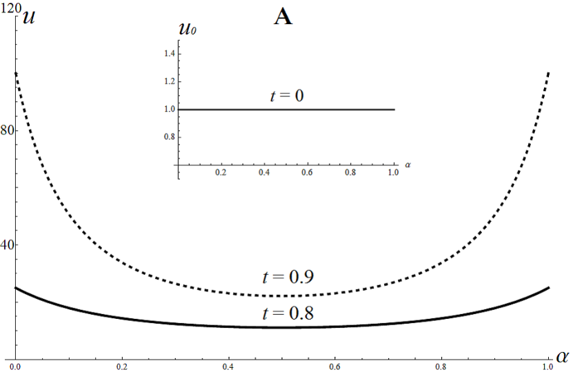
Let u0​(α)≡1u_{0}(\alpha)\equiv 1, f⁡(α)=2​α−1f(\alpha)=2\alpha-1 and g⁡(t)=2​t+1g(t)=2t+1. Then (2.14) and (2.7) give

ψ0​(α)=α2−α,G⁡(t)=t2+t.\psi_{0}(\alpha)=\alpha^{2}-\alpha,\,\,\,\,\,\,\,\,\,\,\,\,G(t)=t^{2}+t.

Note that ψ0≤0\psi_{0}\leq 0, so that M0=0M_{0}=0. Using (2.17), we obtain

u⁡(α,t)=2​t+1(1−α​t2​(t+1)​(α−1))2.u(\alpha,t)=\frac{2t+1}{\left(1-\frac{\alpha t}{2}(t+1)(\alpha-1)\right)^{2}}. (6.1)

The solution remains finite, and positive, for all α∈[0,1]\alpha\in[0,1] and 0≤t<+∞0\leq t<+\infty, whereas

limt→+∞u⁡(α,t)={0,α∈(0,1),+∞,α∈{0,1}.\lim_{t\to+\infty}u(\alpha,t)=\begin{cases}0,\,\,\,\,\,\,\,\,\,\,\,\,\,\,&\alpha\in(0,1),\\ +\infty,\,\,\,\,\,\,\,\,\,\,&\alpha\in\{0,1\}.\end{cases} (6.2)

See Figure (1)(A) below.

6.2. Example 2 - Finite-time Blow-up and Smooth Boundary Data

Consider the same initial and boundary data as in Example 1, but now take f⁡(α)=1−2​αf(\alpha)=1-2\alpha. Then (2.14) becomes ψ0​(α)=α−α2\psi_{0}(\alpha)=\alpha-\alpha^{2} with M0=1/4M_{0}=1/4 attained at α¯1=1/2\overline{\alpha}_{1}=1/2. The solution (2.17) now reads

u⁡(α,t)=2​t+1(1−α​t2​(t+1)​(1−α))2.u(\alpha,t)=\frac{2t+1}{\left(1-\frac{\alpha t}{2}(t+1)(1-\alpha)\right)^{2}}. (6.3)

Since G⁡(t)=t2+tG(t)=t^{2}+t, we solve G⁡(t)=8G(t)=8 and find that t∗=12​(33−1)∼2.37.t_{*}=\frac{1}{2}\left(\sqrt{33}-1\right)\sim 2.37. Using (6.3) we conclude that

limt→t∗u⁡(α,t)={+∞,α=α¯1,33(1−2​α)4,α≠α¯1.\lim_{t\to t_{*}}u(\alpha,t)=\begin{cases}+\infty,\,\,\,\,\,\,\,\,\,\,\,\,\,\,&\alpha=\overline{\alpha}_{1},\\ \frac{\sqrt{33}}{(1-2\alpha)^{4}},\,\,\,\,\,\,\,\,\,\,&\alpha\neq\overline{\alpha}_{1}.\end{cases} (6.4)

See Figure (1)(B) below.

Refer to caption
Refer to caption
Figure 1. For Example 1 above, Figure A depicts the global-in-time behaviour of (6.1), while B represents finite-time blowup of uu in (6.3) as t↑t∗∼2.37t\uparrow t_{*}\sim 2.37.

The following two Examples are instances of Theorem 4.5.

6.3. Example 3 - Induced Boundary Blow-up for M0=0M_{0}=0

For u0u_{0} and ff as in Example 1, let g⁡(t)=(1−t)−2g(t)=(1-t)^{-2}. This implies that M0=0M_{0}=0 occurs only at the boundary points. Then using (4.17), we obtain

u⁡(α,t)=4(2−t⁡(α2−α+2))2,u(\alpha,t)=\frac{4}{(2-t(\alpha^{2}-\alpha+2))^{2}}, (6.5)

which diverges earliest, at the boundary points α¯i={0,1}\overline{\alpha}_{i}=\{0,1\}, as t↑tb=1t\uparrow t_{b}=1. In contrast, for α∈(0,1)\alpha\in(0,1), uu remains finite (and positive) for all t∈[0,1]t\in[0,1]. In fact,

limt↑1u⁡(α,t)=4(α2−α)2,α∈(0,1).\lim_{t\uparrow 1}u(\alpha,t)=\frac{4}{(\alpha^{2}-\alpha)^{2}},\,\,\,\,\,\,\,\,\,\,\,\,\,\,\,\,\alpha\in(0,1).

See Figure 2(A) below.

6.4. Example 4 - Earlier Interior Blowup for M0>0M_{0}>0 with Singular g⁡(t)g(t)

Take u0u_{0} and ff as in Example 2 and g⁡(t)=(1−t)−2g(t)=(1-t)^{-2}. Then we now have M0=1/4M_{0}=1/4 occurring at α¯1=1/2\overline{\alpha}_{1}=1/2. From (4.17), we obtain

u⁡(α,t)=4(2+t⁡(α2−α−2))2,u(\alpha,t)=\frac{4}{(2+t(\alpha^{2}-\alpha-2))^{2}}, (6.6)

which diverges earliest at α=α¯1\alpha=\overline{\alpha}_{1} as

t↑t∗=22+M0=89<tb=1.t\uparrow t_{*}=\frac{2}{2+M_{0}}=\frac{8}{9}<t_{b}=1.

In contrast, for α≠α¯1\alpha\neq\overline{\alpha}_{1}, uu remains finite and positive for all t∈[0,t∗]t\in[0,t_{*}]. In this case, the final solution profile is given by

limt↑t∗u⁡(α,t)=(91−4​α+4​α2)2,α∈[0,1]\{α¯1}.\lim_{t\uparrow t_{*}}u(\alpha,t)=\left(\frac{9}{1-4\alpha+4\alpha^{2}}\right)^{2},\,\,\,\,\,\,\,\,\,\,\,\,\,\,\,\,\alpha\in[0,1]\backslash\{\overline{\alpha}_{1}\}.

See Figure 2(B) below.

Refer to caption
Refer to caption
Figure 2. Blowup profiles for Examples 4 and 5 with singular boundary data. Figure A represents earliest blowup of (6.5) at the boundary as t↑tb=1t\uparrow t_{b}=1 in the case where M0=0M_{0}=0, whereas, for M0>0M_{0}>0, Figure B depicts earliest blowup of (6.6) in the interior as t↑t∗<tbt\uparrow t_{*}<t_{b}.

References

  • [1] M. Chuaqui, P. Duren and B. Osgood, The Schwarzian derivative for harmonic mappings, Journal D’Analyse Mathematique, 91, (2003) 329-351.
  • [2] D.G. Crowdy, General solutions to the 2D Liouville equation, Int. J. Engng Sci., 35 2, (1997) 141-149.
  • [3] D.G. Crowdy, Stuart vortices on a sphere, J. Fluid Mech., 498, (2004) 381-402.
  • [4] G.P. Dzhordzhadze, Regular solutions of the Liouville equation, Theor. Math. Phys+, 41 1, (1979) 867-871
  • [5] G. P. Dzhordzhadze, A. K. Pogrebkov, and M. K. Polivanov, On the solutions with singularities of the Liouville equation, Dokl. Akad. Nauk SSSR, 243, 318 (1978).
  • [6] B. Khesin, J. Lenells and G. Misiolek, Generalized Hunter-Saxton equation and the geometry of the group of circle diffeomorphisms, Math. Ann. 342(3), (2008), 617-656.
  • [7] S. Kichenassamy and W. Littman, Blow-up surfaces for nonlinear wave equations, I, Comm. PDE 18, No. 3&\&4, 431-452 (1993).
  • [8] J. Liouville, J. Math. Pures Appl., 18, 71 (1853).
  • [9] H. Okamoto, Well-posedness of the generalized Proudman-Johnson equation without viscosity, J. Math. Fluid Mech. 11 (2009), 46-59.
  • [10] A.K. Pogrebkov, Global solutions of Cauchy problems for the Liouville equation ϕt​t−ϕx​x=−m22​eϕ\phi_{tt}-\phi_{xx}=-\frac{m^{2}}{2}e^{\phi} in the case of singular initial data, Dokl. Akad. Nauk SSSR, 244, 873 (1979).
  • [11] A.K. Pogrebkov, Complete integrability of dynamical systems generated by singular solutions of liouville’s equation, Theor. Math. Phys.+, 45 2, (1980) 951-957.
  • [12] C. Rogers and W. K. Schief, Ba¨\ddot{a}cklund and Darboux Transformations: Geometry and Modern Applications in Soliton Theory, Cambridge texts in applied mathematics, (2002).
  • [13] B. Ruf and P. Ubilla, On a Liouville-type equation with sign-changing weight, Proceedings of the Royal Society of Edinburg, Sect. A, 139 (2009), 183-192
  • [14] A. Sarria and R. Saxton, Blow-up of solutions to the generalized inviscid Proudman-Johnson equation, J Math Fluid Mech, 15, 3 (2013), 493-523.
  • [15] J.T. Stuart, Fluid. Mech., (1967), 29, 417.
  • [16] M. Wunsch, The generalized Proudman-Johnson equation revisited, J. Math. Fluid Mech. 13 (1), (2009), 147-154.