跳到论文正文
W Papers独立论文阅读器 arXiv:1410.0729 论文正文 计算阅读时间 · 0%
引用这篇论文根据当前论文元数据生成,正式投稿前建议核对。


License: arXiv.org perpetual non-exclusive license
arXiv:1410.0729v2 [math.GT] 26 May 2015

Hitchin characters and geodesic laminationsThanks: This research was partially supported by the grants DMS-0604866 and DMS-1105402 from the U.S. National Science Foundation, and by a Fellowship from the Simons Foundation (grant 301050). In addition, the authors gratefully acknowledge support from the NSF grants DMS-1107452, 1107263 and 1107367 “RNMS: GEometric structures And Representation varieties” (the GEAR Network).

Francis Bonahon Address: Department of Mathematics, University of Southern California, KAP 108, Los Angeles, CA 90089-2532, U.S.A. Email address: fbonahon@math.usc.edu and Guillaume Dreyer Address: Department of Mathematics, University of Notre Dame, 255 Hurley Hall, Notre Dame, IN 46556, U.S.A. Email address: dreyfactor@gmail.com
Date: August 24, 2026
Abstract.

For a closed surface SS, the Hitchin component Hitn​(S)\mathrm{Hit}_{\mathrm{n}}(S) is a preferred component of the character variety consisting of group homomorphisms from the fundamental group π1​(S)\pi_{1}(S) to the Lie group PSLn​(ℝ)\mathrm{PSL_{n}(\mathbb{R})}. We construct a parametrization of the Hitchin component that is well-adapted to a geodesic lamination λ\lambda on the surface. This is a natural extension of Thurston’s parametrization of the Teichmüller space 𝒯⁡(S)\mathcal{T}(S) by shear coordinates associated to λ\lambda, corresponding to the case n=2n=2. However, significantly new ideas are needed in this higher dimensional case. The article concludes with a few applications.

Introduction

0.1. Background and motivation

For a closed, connected, oriented surface SS of genus g>1g>1, the Hitchin component Hitn​(S)\mathrm{Hit}_{\mathrm{n}}(S) is a preferred component of the character variety

𝒳PSLn​(ℝ)(S)={homomorphisms ρ:π1(S)→PSLn(ℝ)}//PSLn(ℝ)\mathcal{X}_{\mathrm{PSL_{n}(\mathbb{R})}}(S)=\{\text{homomorphisms }\rho\colon\pi_{1}(S)\to\mathrm{PSL_{n}(\mathbb{R})}\}/\kern-4.0pt/\mathrm{PSL_{n}(\mathbb{R})}

consisting of group homomorphisms ρ:π1​(S)→PSLn​(ℝ)\rho\colon\pi_{1}(S)\to\mathrm{PSL_{n}(\mathbb{R})} from the fundamental group π1​(S)\pi_{1}(S) to the Lie group PSLn​(ℝ)\mathrm{PSL_{n}(\mathbb{R})} (equal to the special linear group SLn​(ℝ)\mathrm{SL_{n}(\mathbb{R})} if nn is odd, and to SLn​(ℝ)/{±Id}\mathrm{SL_{n}(\mathbb{R})}/\{\pm\mathrm{Id}\} if nn is even), where PSLn​(ℝ)\mathrm{PSL_{n}(\mathbb{R})} acts on these homomorphisms by conjugation. The quotient should normally be taken in the sense of geometric invariant theory [MFK94], but this subtlety is irrelevant here as this quotient construction coincides with the usual topological quotient on the Hitchin component.

When n=2n=2, the Lie group PSL2​(ℝ)\mathrm{PSL}_{2}(\mathbb{R}) is also the orientation-preserving isometry group of the hyperbolic plane ℍ2\mathbb{H}^{2}, and the Hitchin component Hit2​(S)\mathrm{Hit}_{2}(S) of 𝒳PSL2​(ℝ)​(S)\mathcal{X}_{\mathrm{PSL}_{2}(\mathbb{R})}(S) consists of all characters represented by injective homomorphisms ρ:π1​(S)→PSL2​(ℝ)\rho\colon\pi_{1}(S)\to\mathrm{PSL}_{2}(\mathbb{R}) whose image ρ​(π1​(S))\rho\bigl(\pi_{1}(S)\bigr) is discrete in PSL2​(ℝ)\mathrm{PSL}_{2}(\mathbb{R}) and for which the natural homotopy equivalence S→ℍ2/ρ⁡(π1​(S))S\to\mathbb{H}^{2}/\rho\bigl(\pi_{1}(S)\bigr) has degree +1+1. The Hitchin component Hit2​(S)\mathrm{Hit}_{2}(S) is in this case called the Teichmüller component, and can also be described as the space of isotopy classes of hyperbolic metrics on SS.

When n>2n>2, there is a preferred homomorphism PSL2​(ℝ)→PSLn​(ℝ)\mathrm{PSL}_{2}(\mathbb{R})\to\mathrm{PSL_{n}(\mathbb{R})} coming from the unique nn–dimensional representation of SL2​(ℝ)\mathrm{SL}_{2}(\mathbb{R}) (or, equivalently, from the natural action of SL2​(ℝ)\mathrm{SL}_{2}(\mathbb{R}) on the vector space ℝ​[X,Y]n−1≅ℝn\mathbb{R}[X,Y]_{n-1}\cong\mathbb{R}^{n} of homogeneous polynomials of degree n−1n-1 in two variables). This provides a natural map 𝒳PSL2​(ℝ)​(S)→𝒳PSLn​(ℝ)​(S)\mathcal{X}_{\mathrm{PSL}_{2}(\mathbb{R})}(S)\to\mathcal{X}_{\mathrm{PSL_{n}(\mathbb{R})}}(S), and the Hitchin component Hitn​(S)\mathrm{Hit}_{\mathrm{n}}(S) is the component of 𝒳PSLn​(ℝ)​(S)\mathcal{X}_{\mathrm{PSL_{n}(\mathbb{R})}}(S) that contains the image of Hit2​(S)⊂𝒳PSL2​(ℝ)​(S)\mathrm{Hit}_{2}(S)\subset\mathcal{X}_{\mathrm{PSL}_{2}(\mathbb{R})}(S). The terminology is motivated by the following fundamental result of Hitchin [Hit92], who was the first to single out this component.

Theorem 0.1 (Hitchin).

The Hitchin component Hitn​(S)\mathrm{Hit}_{\mathrm{n}}(S) is diffeomorphic to ℝ2​(g−1)​(n2−1)\mathbb{R}^{2(g-1)(n^{2}-1)}.

A Hitchin character is an element of the Hitchin component Hitn​(S)\mathrm{Hit}_{\mathrm{n}}(S), and a Hitchin homomorphism is a homomorphism ρ:π1​(S)→PSLn​(ℝ)\rho\colon\pi_{1}(S)\to\mathrm{PSL_{n}(\mathbb{R})} representing a Hitchin character. We will use the same letter to represent the Hitchin homomorphism ρ:π1​(S)→PSLn​(ℝ)\rho\colon\pi_{1}(S)\to\mathrm{PSL_{n}(\mathbb{R})} and the corresponding Hitchin character ρ∈Hitn​(S)\rho\in\mathrm{Hit}_{\mathrm{n}}(S).

About 15 years after [Hit92], Labourie [Lab06] showed that Hitchin homomorphisms satisfy many important geometric and dynamical properties, and in particular are injective with discrete image; see also [FG06].

Hitchin’s construction of the parametrization of Hitn​(S)\mathrm{Hit}_{\mathrm{n}}(S) given by Theorem 0.1 is based on geometric analysis techniques that provide little information on the geometry of the Hitchin homomorphisms themselves; see [Lof01, Lab07, Lab14] for different geometric analytic parametrizations when n=3n=3. The current article is devoted to developing another parametrization of the Hitchin component Hitn​(S)\mathrm{Hit}_{\mathrm{n}}(S) which is much more geometric, and has the additional advantage of being well-behaved with respect to a geodesic lamination. Geodesic laminations were introduced by Thurston to develop a continuous calculus for simple closed curves on the surface SS, and provide very powerful tools for many topological and geometric problems in dimensions 2 and 3. See §§9 and 10 for two simple applications of our parametrization, one to the dynamics of the action of a pseudo-Anosov homomorphism of SS on the Hitchin component, and another one to the length functions defined by a Hitchin character on Thurston’s space ℳ​ℒ​(S)\mathcal{ML}(S) of measured laminations on SS.

Our construction is a natural extension of Thurston’s parametrization of the Teichmüller component by shear coordinates [Thu86, Bon96]. It draws its inspiration from this classical case where n=2n=2, but also from work of Fock-Goncharov [FG06] on a variant of the Hitchin component where the surface SS has punctures, and where these punctures are endowed with additional information. As in the classical case when n=2n=2, the situation is conceptually and analytically much more complicated for a closed surface than in the case considered in [FG06]. Many arguments, such as those of §§5.1, 6.2 and 8.2, are new even for the case n=2n=2.

The companion article [BD14] is devoted to a special case of our parametrization, when the geodesic lamination has only finitely many leaves. The situation is much simpler in that case, and in particular the arguments of [BD14] tend to be very combinatorial in nature. The current article has a much more analytic flavor. It is also more conceptual, and provides a homological interpretation of some of the invariants and phenomena that were developed in a purely computational way in [BD14]. And of course the framework of general geodesic laminations, possibly with uncountably many leaves, considered in this article is better suited for applications.

The article [Dre13b] was developed, to a large extent, as a first step towards the more general results of the current paper. It investigates all deformations of a Hitchin character ρ∈Hitn​(S)\rho\in\mathrm{Hit}_{\mathrm{n}}(S) that respect its triangle invariants, as discussed in the next section.

0.2. Main results

We can now be more specific. Let λ\lambda be a maximal geodesic lamination in SS. See §2 for precise definitions. What we need to know here is just that, for an arbitrary auxiliary metric of negative curvature on the surface, λ\lambda is decomposed as a union of disjoint geodesic leaves, and that its complement S−λS-\lambda consists of 4​(g−1)4(g-1) infinite triangles with geodesic boundary. Some maximal geodesic laminations, such as the ones considered in [BD14], have only a finite number of leaves, but generic examples have uncountably many leaves.

Given a Hitchin character ρ∈Hitn​(S)\rho\in\mathrm{Hit}_{\mathrm{n}}(S), the rich dynamical structure for ρ\rho discovered by Labourie [Lab06] associates a triple (E,F,G)(E,F,G) of three flags of ℝn\mathbb{R}^{n} to each triangle component TjT_{j} of S−λS-\lambda. In addition, Fock and Goncharov [FG06] prove that this flag triple (E,F,G)(E,F,G) is positive, in a sense discussed in §1.5, and is determined by (n−1)​(n−2)2\frac{(n-1)(n-2)}{2} invariants τa​b​cρ​(E,F,G)∈ℝ\tau_{abc}^{\rho}(E,F,G)\in\mathbb{R}. Since S−λS-\lambda has 4​(g−1)4(g-1) components, these flag triple invariants can be collected into a single triangle invariant τρ∈ℝ2​(g−1)​(n−1)​(n−2)\tau^{\rho}\in\mathbb{R}^{2(g-1)(n-1)(n-2)}.

The really new feature introduced in this article describes how to glue these flag triples across the (possibly uncountably many) leaves of the lamination, and simultaneously involves analytic and combinatorial arguments. The analytic part of this analysis is based on the slithering map constructed in §5.1, which is a higher dimensional analogue of the horocyclic foliation that is at the basis of the case n=2n=2 [Thu86, Bon96]. This slithering map enables us to control the gluing by elements of the homology of a train track neighborhood UU for λ\lambda, which we now briefly describe. The precise definition of train track neighborhoods can be found in §4.2 (and is familiar to experts); at this point, it suffices to say that UU is obtained from SS by removing 2​(g−1)2(g-1) disjoint disks, one in each component of S−λS-\lambda; in addition, the boundary ∂U\partial U is decomposed into a horizontal boundary ∂hU\partial_{\mathrm{h}}U and a vertical boundary ∂vU\partial_{\mathrm{v}}U, in such a way that each component of ∂U\partial U is a hexagon made up of three arc components of ∂hU\partial_{\mathrm{h}}U and three arc components of ∂vU\partial_{\mathrm{v}}U.

The geodesic lamination has a well-defined 2–fold orientation cover λ^\widehat{\lambda}, whose leaves are continuously oriented, and the covering map λ^→λ\widehat{\lambda}\to\lambda uniquely extends to a 2–fold cover U^→U\widehat{U}\to U. In particular, λ^\widehat{\lambda} is a geodesic lamination in the surface U^\widehat{U}.

Our new invariant for a Hitchin character ρ∈Hitn​(S)\rho\in\mathrm{Hit}_{\mathrm{n}}(S) is a certain shearing class [σρ]∈H1​(U^,∂vU^,ℝn−1)[\sigma^{\rho}]\in H_{1}(\widehat{U},\partial_{\mathrm{v}}\widehat{U};\mathbb{R}^{n-1}). This shearing class has the property that ι∗​([σρ])=−[σρ]¯\iota_{*}\bigl([\sigma^{\rho}]\bigr)=-\overline{[\sigma^{\rho}]}, for the covering involution ι\iota of the cover U^→U\widehat{U}\to U and for the involution x↦x¯x\mapsto\overline{x} of ℝn−1\mathbb{R}^{n-1} that associates x¯=(xn−1,xn−2,…,x1)\overline{x}=(x_{n-1},x_{n-2},\dots,x_{1}) to x=(x1,x2,…,xn−1)x=(x_{1},x_{2},\dots,x_{n-1}). In particular, [σρ][\sigma^{\rho}] can also be interpreted as a twisted homology class [σρ]∈H1​(U,∂vU,ℝ~n−1)[\sigma^{\rho}]\in H_{1}(U,\partial_{\mathrm{v}}U;\widetilde{\mathbb{R}}^{n-1}) valued in a suitable coefficient bundle ℝ~n−1\widetilde{\mathbb{R}}^{n-1} over UU with fiber ℝn−1\mathbb{R}^{n-1}.

The triangle invariant τρ∈ℝ2​(g−1)​(n−1)​(n−2)\tau^{\rho}\in\mathbb{R}^{2(g-1)(n-1)(n-2)} and shearing class [σρ]∈H1​(U^,∂vU^,ℝn−1)[\sigma^{\rho}]\in H_{1}(\widehat{U},\partial_{\mathrm{v}}\widehat{U};\mathbb{R}^{n-1}) satisfy two types of constraints. The first constraint is a homological equality.

Proposition 0.2 (Shearing Cycle Boundary Condition).

The boundary ∂[σρ]∈H0​(∂vU^,ℝn−1)\partial[\sigma^{\rho}]\in H_{0}(\partial_{\mathrm{v}}\widehat{U};\mathbb{R}^{n-1}) of the shearing class [σρ]∈H1​(U^,∂vU^,ℝn−1)[\sigma^{\rho}]\in H_{1}(\widehat{U},\partial_{\mathrm{v}}\widehat{U};\mathbb{R}^{n-1}) of a Hitchin character ρ∈Hitn​(S)\rho\in\mathrm{Hit}_{\mathrm{n}}(S) is completely determined by the triangle invariant τρ∈ℝ2​(g−1)​(n−1)​(n−2)\tau^{\rho}\in\mathbb{R}^{2(g-1)(n-1)(n-2)}, by an explicit linear formula given in §5.2.

The second constraint is a positivity property, proved as Corollary 7.10 in §7.2. Because the leaves of the orientation cover λ^\widehat{\lambda} are oriented, a famous construction of Ruelle and Sullivan [RS75] interprets every transverse measure μ\mu for the orientation cover λ^\widehat{\lambda} as a 1–dimensional de Rham current in U^\widehat{U}. In particular, such a transverse measure μ\mu determines a homology class [μ]∈H1​(U^,ℝ)[\mu]\in H_{1}(\widehat{U};\mathbb{R}).

Proposition 0.3 (Positive Intersection Condition).

For every transverse measure μ\mu for the orientation cover λ^\widehat{\lambda}, the algebraic intersection vector [μ]⋅[σρ]∈ℝn−1[\mu]\cdot[\sigma^{\rho}]\in\mathbb{R}^{n-1} of the shearing class [σρ]∈H1​(U^,∂vU^,ℝn−1)[\sigma^{\rho}]\in H_{1}(\widehat{U},\partial_{\mathrm{v}}\widehat{U};\mathbb{R}^{n-1}) with [μ]∈H1​(U^,ℝ)[\mu]\in H_{1}(\widehat{U};\mathbb{R}) is positive, in the sense that all its coordinates are positive.

The Shearing Cycle Boundary and Positive Intersection Conditions restrict the pair (τρ,[σρ])\bigl(\tau^{\rho},[\sigma^{\rho}]\bigr) to a convex polyhedral cone 𝒫\mathcal{P} in ℝ2​(g−1)​(n−1)​(n−2)×H1​(U^,∂vU^,ℝn−1)\mathbb{R}^{2(g-1)(n-1)(n-2)}\times H_{1}(\widehat{U},\partial_{\mathrm{v}}\widehat{U};\mathbb{R}^{n-1}). The main result of the article, proved as Theorem 8.13 in §8.3, shows that these are the only restrictions on the triangle and shearing invariants, and that these provide a parametrization of the Hitchin component Hitn​(S)\mathrm{Hit}_{\mathrm{n}}(S).

Theorem 0.4 (Parametrization of the Hitchin component).

The map Hitn​(S)→𝒫\mathrm{Hit}_{\mathrm{n}}(S)\to\mathcal{P}, which to a Hitchin character ρ∈Hitn​(S)\rho\in\mathrm{Hit}_{\mathrm{n}}(S) associates the pair (τρ,[σρ])\bigl(\tau^{\rho},[\sigma^{\rho}]\bigr) formed by its triangle invariant τρ∈ℝ2​(g−1)​(n−1)​(n−2)\tau^{\rho}\in\mathbb{R}^{2(g-1)(n-1)(n-2)} and its shearing class [σρ]∈H1​(U^,∂vU^,ℝn−1)[\sigma^{\rho}]\in H_{1}(\widehat{U},\partial_{\mathrm{v}}\widehat{U};\mathbb{R}^{n-1}), is a homeomorphism.

The Shearing Cycle Boundary Condition provides some unexpected constraints on the triangle invariants of Hitchin characters, as well as on their shearing classes. The following two statements are abbreviated expressions of more specific computations given in §8.4. These restrictions are somewhat surprising when one considers the relatively large dimension 2​(g−1)​(n2−1)2(g-1)(n^{2}-1) of Hitn​(S)\mathrm{Hit}_{\mathrm{n}}(S).

Proposition 0.5.

An element τ∈ℝ2​(g−1)​(n−1)​(n−2)\tau\in\mathbb{R}^{2(g-1)(n-1)(n-2)} is the triangle invariant τρ\tau^{\rho} of a Hitchin character ρ∈Hitn​(S)\rho\in\mathrm{Hit}_{\mathrm{n}}(S) if and only if it belongs to a certain explicit subspace of codimension ⌊n−12⌋\lfloor\frac{n-1}{2}\rfloor of ℝ2​(g−1)​(n−1)​(n−2)\mathbb{R}^{2(g-1)(n-1)(n-2)}.

Proposition 0.6.

A relative homology class [σ]∈H1​(U^,∂vU^,ℝn−1)[\sigma]\in H_{1}(\widehat{U},\partial_{\mathrm{v}}\widehat{U};\mathbb{R}^{n-1}) is the shearing class [σρ][\sigma^{\rho}] of a Hitchin character ρ∈Hitn​(S)\rho\in\mathrm{Hit}_{\mathrm{n}}(S) if and only if it belongs to a certain open convex polyhedral cone in an explicit linear subspace of dimension 6​(g−1)​(3​n−7)6(g-1)(3n-7) if n>3n>3, of dimension 16​(g−1)16(g-1) if n=3n=3, and of dimension 6​(g−1)6(g-1) if n=2n=2.

The dimensions in Proposition 0.6 should be compared to the dimension 18​(g−1)​(n−1)18(g-1)(n-1) of the twisted homology space H1​(U,∂vU,ℝ~n−1)H_{1}(U,\partial_{\mathrm{v}}U;\widetilde{\mathbb{R}}^{n-1}), consisting of those α∈H1​(U^,∂vU^,ℝn−1)\alpha\in H_{1}(\widehat{U},\partial_{\mathrm{v}}\widehat{U};\mathbb{R}^{n-1}) such that ι∗​(α)=−α¯\iota_{*}(\alpha)=-\overline{\alpha}.

At first, the relative homology group H1​(U^,∂vU^,ℝn−1)H_{1}(\widehat{U},\partial_{\mathrm{v}}\widehat{U};\mathbb{R}^{n-1}) of a train track neighborhood UU may not appear very natural. In fact, although we decided to privilege this more familiar point of view in this introduction, it occurs as a space 𝒞⁡(λ^,slits,ℝn−1)\mathcal{C}(\widehat{\lambda},\mathrm{slits};\mathbb{R}^{n-1}) of tangent cycles for the orientation cover λ^\widehat{\lambda} relative to its slits, where the slits of λ^\widehat{\lambda} are lifts of the spikes of the complement S−λS-\lambda; Proposition 4.5 then provides an isomorphism 𝒞⁡(λ^,slits,ℝn−1)≅H1​(U^,∂vU^,ℝn−1)\mathcal{C}(\widehat{\lambda},\mathrm{slits};\mathbb{R}^{n-1})\cong H_{1}(\widehat{U},\partial_{\mathrm{v}}\widehat{U};\mathbb{R}^{n-1}). A relative tangent cycle α∈𝒞⁡(λ^,slits,ℝn−1)\alpha\in\mathcal{C}(\widehat{\lambda},\mathrm{slits};\mathbb{R}^{n-1}) assigns a vector α⁡(k)∈ℝn−1\alpha(k)\in\mathbb{R}^{n-1} to each arc kk transverse to λ^\widehat{\lambda}, in a quasi-additive way: If kk is split into two subarcs k1k_{1} and k2k_{2}, then α⁡(k)\alpha(k) is equal to the sum of α⁡(k1)\alpha(k_{1}), α⁡(k2)\alpha(k_{2}) and of a correction factor depending on the slit of λ^\widehat{\lambda} facing the point k1∩k2k_{1}\cap k_{2} along which kk was split. In particular, 𝒞⁡(λ^,slits,ℝn−1)\mathcal{C}(\widehat{\lambda},\mathrm{slits};\mathbb{R}^{n-1}) depends only on the maximal geodesic lamination λ\lambda, and not on the train track neighborhood UU.

The lack of additivity of a relative tangent cycle α∈𝒞⁡(λ^,slits,ℝn−1)\alpha\in\mathcal{C}(\widehat{\lambda},\mathrm{slits};\mathbb{R}^{n-1}) has a nice expression in terms of the boundary map ∂:H1​(U^,∂vU^,ℝn−1)→H0​(∂vU^,ℝn−1)\partial\colon H_{1}(\widehat{U},\partial_{\mathrm{v}}\widehat{U};\mathbb{R}^{n-1})\to H_{0}(\partial_{\mathrm{v}}\widehat{U};\mathbb{R}^{n-1}), and is at the basis of the Shearing Cycle Boundary Condition of Proposition 0.2. In the classical case where n=2n=2, the Shearing Cycle Boundary Condition says that the shearing class [σρ]∈H1​(U^,∂vU^,ℝn−1)[\sigma^{\rho}]\in H_{1}(\widehat{U},\partial_{\mathrm{v}}\widehat{U};\mathbb{R}^{n-1}) has boundary 0, and in particular that the corresponding tangent cycle [σρ]∈𝒞⁡(λ^,slits,ℝ)[\sigma^{\rho}]\in\mathcal{C}(\widehat{\lambda},\mathrm{slits};\mathbb{R}) is additive with no correction factors; such objects were called “transverse cocycles” in [Bon97b, Bon96].

This point of view enables us to shed some light on the Positive Intersection Condition of Proposition 0.3. Given a Hitchin character ρ∈Hitn​(S)\rho\in\mathrm{Hit}_{\mathrm{n}}(S), Labourie [Lab06] shows that for every nontrivial γ∈π1​(S)\gamma\in\pi_{1}(S) the matrix ρ​(γ)∈PSLn​(ℝ)\rho(\gamma)\in\mathrm{PSL_{n}(\mathbb{R})} is diagonalizable, and that its eigenvalues maρ​(γ)m_{a}^{\rho}(\gamma) can be ordered in such a way that |m1ρ​(γ)|>|m2ρ​(γ)|>⋯>|mnρ​(γ)||m_{1}^{\rho}(\gamma)|>|m_{2}^{\rho}(\gamma)|>\dots>|m_{n}^{\rho}(\gamma)|. If we define ℓρ​(γ)∈ℝn−1\ell^{\rho}(\gamma)\in\mathbb{R}^{n-1} by the property that its aa–th coordinate is ℓaρ​(γ)=log⁡|maρ​(γ)||ma+1ρ​(γ)|\ell^{\rho}_{a}(\gamma)=\log\frac{|m_{a}^{\rho}(\gamma)|}{|m_{a+1}^{\rho}(\gamma)|}, the second author showed in [Dre13a] that this formula admits a continuous linear extension ℓρ:𝒞H​o¨​l​(S)→ℝn−1\ell^{\rho}\colon\mathcal{C}^{\mathrm{H{\ddot{o}}l}}(S)\to\mathbb{R}^{n-1} to the space 𝒞H​o¨​l​(S)\mathcal{C}^{\mathrm{H{\ddot{o}}l}}(S) of Hölder geodesic currents of SS, a topological vector space that contains all conjugacy classes of π1​(S)\pi_{1}(S) in a natural way; this continuous extension ℓρ:𝒞H​o¨​l​(S)→ℝn−1\ell^{\rho}\colon\mathcal{C}^{\mathrm{H{\ddot{o}}l}}(S)\to\mathbb{R}^{n-1} is unique on the subspaces of 𝒞H​o¨​l​(S)\mathcal{C}^{\mathrm{H{\ddot{o}}l}}(S) that are of interest to us in this paper (see Remark 7.3).

In particular, an (additive) tangent cycle α∈𝒞⁡(λ^,ℝ)\alpha\in\mathcal{C}(\widehat{\lambda};\mathbb{R}) defines a Hölder geodesic current α∈𝒞H​o¨​l​(S)\alpha\in\mathcal{C}^{\mathrm{H{\ddot{o}}l}}(S) (see [Bon97b]), and we can restrict the length function of [Dre13a] to ℓρ:𝒞⁡(λ^,ℝ)→ℝn−1\ell^{\rho}\colon\mathcal{C}(\widehat{\lambda};\mathbb{R})\to\mathbb{R}^{n-1}.

The following result, proved as Theorem 7.5 in §7.2, relates the length vector ℓρ​(α)∈ℝn−1\ell^{\rho}(\alpha)\in\mathbb{R}^{n-1} to the shearing class [σρ]∈𝒞⁡(λ^,slits,ℝn−1)≅H1​(U^,∂vU^,ℝn−1)[\sigma^{\rho}]\in\mathcal{C}(\widehat{\lambda},\mathrm{slits};\mathbb{R}^{n-1})\cong H_{1}(\widehat{U},\partial_{\mathrm{v}}\widehat{U};\mathbb{R}^{n-1}).

Theorem 0.7 (Length and Intersection Formula).

If [σρ]∈𝒞⁡(λ^,slits,ℝn−1)≅H1​(U^,∂vU^,ℝn−1)[\sigma^{\rho}]\in\mathcal{C}(\widehat{\lambda},\mathrm{slits};\mathbb{R}^{n-1})\cong H_{1}(\widehat{U},\partial_{\mathrm{v}}\widehat{U};\mathbb{R}^{n-1}) is the shearing cycle of a Hitchin character ρ∈Hitn​(S)\rho\in\mathrm{Hit}_{\mathrm{n}}(S), and if α∈𝒞⁡(λ^,ℝ)≅H1​(U^,ℝ)\alpha\in\mathcal{C}(\widehat{\lambda};\mathbb{R})\cong H_{1}(\widehat{U};\mathbb{R}) is a tangent cycle for the orientation cover λ^\widehat{\lambda}, then

ℓaρ​(α)=[α]⋅[σρ]∈ℝn−1\ell_{a}^{\rho}(\alpha)=[\alpha]\cdot[\sigma^{\rho}]\in\mathbb{R}^{n-1}

is the algebraic intersection vector of the homology classes [α]∈H1​(U^,ℝ)[\alpha]\in H_{1}(\widehat{U};\mathbb{R}) and [σρ]∈H1​(U^,∂vU^,ℝn−1)[\sigma^{\rho}]\in H_{1}(\widehat{U},\partial_{\mathrm{v}}\widehat{U};\mathbb{R}^{n-1}) in the train track neighborhood U^\widehat{U} of λ^\widehat{\lambda}.

In the special case where α\alpha is a transverse measure μ\mu for λ^\widehat{\lambda}, the Positive Intersection Condition of Proposition 0.3 is then equivalent to the property that all coordinates of the vector ℓρ​(μ)\ell^{\rho}(\mu) are positive. In this version, this statement is an immediate consequence of the Anosov Property that is central to [Lab06] (see Proposition 7.4).

The article concludes, in §§9 and 10, with two brief applications of Theorems 0.4 and 0.7. The first one is concerned with the dynamics of the action of a pseudo-Anosov diffeomorphism φ:S→S\varphi\colon S\to S on the Hitchin component Hitn​(S)\mathrm{Hit}_{\mathrm{n}}(S); applying the parametrization of Theorem 0.4 to the case of a maximal geodesic lamination λ\lambda containing the stable lamination of φ\varphi shows that the dynamics of the action of φ\varphi on Hitn​(S)\mathrm{Hit}_{\mathrm{n}}(S) are concentrated on submanifolds of Hitn​(S)\mathrm{Hit}_{\mathrm{n}}(S) of relatively large codimension. The second application considers the restriction of the length function ℓρ:𝒞H​o¨​l​(S)→ℝn−1\ell^{\rho}\colon\mathcal{C}^{\mathrm{H{\ddot{o}}l}}(S)\to\mathbb{R}^{n-1} to Thurston’s space ℳ​ℒ​(S)\mathcal{ML}(S) of measured laminations on SS; a consequence of Theorem 0.7 is that, at each α∈ℳ​ℒ​(S)\alpha\in\mathcal{ML}(S), the tangent map Tα​ℓρ:Tα​ℳ​ℒ​(S)→ℝn−1T_{\alpha}\ell^{\rho}\colon T_{\alpha}\mathcal{ML}(S)\to\mathbb{R}^{n-1} is linear on each face of the piecewise linear structure of ℳ​ℒ​(S)\mathcal{ML}(S).

These results can be put in a broader perspective. Indeed, the properties of the Hitchin component remain valid when the Lie group PSLn​(ℝ)\mathrm{PSL_{n}(\mathbb{R})} is replaced by any split real algebraic group GG [Hit92, Lab06, FG06]. In this more general framework, our triangle invariant τρ\tau^{\rho} associates to each component of S−λS-\lambda a positive triple in the flag space B\GB\backslash G, where BB is a Borel subgroup. The shearing class is now a relative homology class [σρ]∈H1​(U^,∂vU^,𝔥)[\sigma^{\rho}]\in H_{1}(\widehat{U},\partial_{\mathrm{v}}\widehat{U};\mathfrak{h}) valued in the Cartan algebra 𝔥\mathfrak{h} of GG, and equivariant with respect to the covering involution ι:U^→U^\iota\colon\widehat{U}\to\widehat{U} and to minus the opposition involution of 𝔥\mathfrak{h}. The Shearing Cycle Boundary Condition then states that the boundary ∂[σρ]∈H0​(∂vU^,𝔥)\partial[\sigma^{\rho}]\in H_{0}(\partial_{\mathrm{v}}\widehat{U};\mathfrak{h}) is completely determined by the triangle invariant τρ∈(B\G)4​(g−1)\tau^{\rho}\in(B\backslash G)^{4(g-1)}, while the Positive Intersection Condition requires that the algebraic intersection vector [μ]⋅[σρ]∈𝔥[\mu]\cdot[\sigma^{\rho}]\in\mathfrak{h} belong to the principal Weyl chamber of 𝔥\mathfrak{h}. The output of these constructions is perhaps not as explicit as in the case of PSLn​(ℝ)\mathrm{PSL_{n}(\mathbb{R})}, but extending the proofs to this more general context is only a matter of using the right vocabulary.

Acknowledgement: The authors are very pleased to acknowledge very helpful conversations with Antonin Guilloux and Anne Parreau, at a time when they (the authors) were very confused. They are also grateful to Giuseppe Martone for many useful comments on the manuscript.

1. Generic configurations of flags

Flags in ℝn\mathbb{R}^{n} play a fundamental rôle in our construction of invariants of Hitchin characters. This section is devoted to certain invariants of finite families of flags, borrowed from [FG06].

1.1. Flags

A flag in ℝn\mathbb{R}^{n} is a family FF of nested linear subspaces F(0)⊂F(1)⊂⋯⊂F(n−1)⊂F(n)F^{(0)}\subset F^{(1)}\subset\dots\subset F^{(n-1)}\subset F^{(n)} of ℝn\mathbb{R}^{n} where each F(a)F^{(a)} has dimension aa.

A pair of flags (E,F)(E,F) is generic if every subspace E(a)E^{(a)} of EE is transverse to every subspace F(b)F^{(b)} of FF. This is equivalent to the property that E(a)∩F(n−a)=0E^{(a)}\cap F^{(n-a)}=0 for every aa.

Similarly, a triple of flags (E,F,G)(E,F,G) is generic if each triple of subspaces E(a)E^{(a)}, F(b)F^{(b)}, G(c)G^{(c)}, respectively in EE, FF, GG, meets transversely. Again, this is equivalent to the property that E(a)∩F(b)∩G(c)=0E^{(a)}\cap F^{(b)}\cap G^{(c)}=0 for every aa, bb, cc with a+b+c=na+b+c=n.

1.2. Wedge-product invariants of generic flag triples

Elementary linear algebra shows that, for any two generic flag pairs (E,F)(E,F) and (E′,F′)(E^{\prime},F^{\prime}), there is a linear isomorphism ℝn→ℝn\mathbb{R}^{n}\to\mathbb{R}^{n} sending EE to E′E^{\prime} and FF to F′F^{\prime}. However, the same is not true for generic flag triples. Indeed, there is a whole moduli space of generic flag triples modulo the action of GLn​(ℝ)\mathrm{GL_{n}(\mathbb{R})}, and this moduli space can be parametrized by invariants that we now describe. These invariants are expressed in terms of the exterior algebra Λ∙​(ℝn)\Lambda^{\bullet}(\mathbb{R}^{n}) of ℝn\mathbb{R}^{n}.

Consider the discrete triangle

Θn={(a,b,c)∈ℤ3;a+b+c=n and a,b,c⩾0}.\Theta_{n}=\{(a,b,c)\in\mathbb{Z}^{3};a+b+c=n\text{ and }a,b,c\geqslant 0\}.

represented in Figure 1.

\SetLabels

R(- 0*-.15) (n,0,0)(n,0,0)
(.5* 1.08) (0,n,0)(0,n,0)
Ł( 1* -.15) (0,0,n)(0,0,n)
( * )
( * )
\endSetLabels

\AffixLabelsRefer to caption

Figure 1. The discrete triangle Θn\Theta_{n}, with a hexagon cycle

A function φ:Θn→ℤ\varphi\colon\Theta_{n}\to\mathbb{Z} is balanced if, for every a0a_{0}, b0b_{0}, c0c_{0},

∑(a0,b,c)∈Θnφ⁡(a0,b,c)=∑(a,b0,c)∈Θnφ⁡(a,b0,c)=∑(a,b,c0)∈Θnφ⁡(a,b,c0)=0,\sum_{(a_{0},b,c)\in\Theta_{n}}\varphi(a_{0},b,c)=\sum_{(a,b_{0},c)\in\Theta_{n}}\varphi(a,b_{0},c)=\sum_{(a,b,c_{0})\in\Theta_{n}}\varphi(a,b,c_{0})=0,

namely if the sum of the φ⁡(a,b,c)\varphi(a,b,c) over each line parallel to one side of the triangle Θn\Theta_{n} is equal to 0.

Such a balanced function φ\varphi defines an invariant of a generic flag triple (E,F,G)(E,F,G) as follows. For each aa, bb, cc between 00 and nn, the spaces Λa​(E(a))\Lambda^{a}\bigl(E^{(a)}\bigr), Λb​(F(b))\Lambda^{b}\bigl(F^{(b)}\bigr) and Λc​(G(c))\Lambda^{c}\bigl(G^{(c)}\bigr) are each isomorphic to ℝ\mathbb{R}. Choose non-zero elements e(a)∈Λa​(E(a))e^{(a)}\in\Lambda^{a}\bigl(E^{(a)}\bigr), f(b)∈Λb(F(b))f^{(b)}\in\Lambda^{b}\bigr(F^{(b)}\bigr) and g(c)∈Λc​(G(c))g^{(c)}\in\Lambda^{c}\bigl(G^{(c)}\bigr). We will use the same letters to denote their images e(a)∈Λa​(ℝn)e^{(a)}\in\Lambda^{a}(\mathbb{R}^{n}), f(b)∈Λb​(ℝn)f^{(b)}\in\Lambda^{b}(\mathbb{R}^{n}) and g(c)∈Λc​(ℝn)g^{(c)}\in\Lambda^{c}(\mathbb{R}^{n}). We then define

Φ⁡(E,F,G)=∏(a,b,c)∈Θn(e(a)∧f(b)∧g(c))φ⁡(a,b,c)∈ℝ,\Phi(E,F,G)=\prod_{(a,b,c)\in\Theta_{n}}\bigl(e^{(a)}\wedge f^{(b)}\wedge g^{(c)}\bigr)^{\varphi(a,b,c)}\in\mathbb{R},

where we choose an isomorphism Λn​(ℝn)≅ℝ\Lambda^{n}(\mathbb{R}^{n})\cong\mathbb{R} to interpret each term in the product as a real number. The fact that the flag triple is generic guarantees that these numbers are non-zero, while the property that φ\varphi is balanced is exactly what is needed to make sure that this product is independent of the choices of the elements e(a)∈Λa​(E(a))e^{(a)}\in\Lambda^{a}\bigl(E^{(a)}\bigr), f(b)∈Λb(F(b))f^{(b)}\in\Lambda^{b}\bigr(F^{(b)}\bigr) and g(c)∈Λc​(G(c))g^{(c)}\in\Lambda^{c}\bigl(G^{(c)}\bigr) and of the isomorphism Λn​(ℝn)≅ℝ\Lambda^{n}(\mathbb{R}^{n})\cong\mathbb{R}. We say that Φ\Phi is the wedge-product invariant of generic flag triples associated to the balanced function φ:Θ→ℤ\varphi\colon\Theta\to\mathbb{Z}.

We now consider a fundamental special case. For aa, bb, c⩾1c\geqslant 1 with a+b+c=na+b+c=n, namely for a point (a,b,c)(a,b,c) in the interior of the triangle Θn\Theta_{n}, the (a,b,c)(a,b,c)–hexagon cycle is the balanced function φa​b​c:Θn→ℤ\varphi_{abc}\colon\Theta_{n}\to\mathbb{Z} defined by

φa​b​c=δ(a+1,b,c−1)−δ(a−1,b,c+1)+δ(a,b−1,c+1)−δ(a,b+1,c−1)+δ(a−1,b+1,c)−δ(a+1,b−1,c),\varphi_{abc}=\delta_{(a+1,b,c-1)}-\delta_{(a-1,b,c+1)}+\delta_{(a,b-1,c+1)}-\delta_{(a,b+1,c-1)}+\delta_{(a-1,b+1,c)}-\delta_{(a+1,b-1,c)},

where δ(a,b,c):Θn→ℤ\delta_{(a,b,c)}\colon\Theta_{n}\to\mathbb{Z} denotes the Kronecker function such that δ(a,b,c)​(a′,b′,c′)=1\delta_{(a,b,c)}(a^{\prime},b^{\prime},c^{\prime})=1 if (a,b,c)=(a′,b′,c′)(a,b,c)=(a^{\prime},b^{\prime},c^{\prime}) and δ(a,b,c)​(a′,b′,c′)=0\delta_{(a,b,c)}(a^{\prime},b^{\prime},c^{\prime})=0 otherwise. The terminology is explained by the fact that the support of φa​b​c\varphi_{abc} is a small hexagon in the discrete triangle Θn\Theta_{n}, centered at the point (a,b,c)(a,b,c); see Figure 1 for the case where n=9n=9 and (a,b,c)=(2,3,4)(a,b,c)=(2,3,4). The wedge-product invariant associated to the hexagon cycle φa​b​c\varphi_{abc} is the (a,b,c)(a,b,c)–triple ratio

Ta​b​c​(E,F,G)\displaystyle T_{abc}(E,F,G) =e(a+1)∧f(b)∧g(c−1)e(a−1)∧f(b)∧g(c+1)\displaystyle=\frac{e^{(a+1)}\wedge f^{(b)}\wedge g^{(c-1)}}{e^{(a-1)}\wedge f^{(b)}\wedge g^{(c+1)}}
e(a)∧f(b−1)∧g(c+1)e(a)∧f(b+1)∧g(c−1)e(a−1)∧f(b+1)∧g(c)e(a+1)∧f(b−1)∧g(c).\displaystyle\qquad\qquad\qquad\qquad\frac{e^{(a)}\wedge f^{(b-1)}\wedge g^{(c+1)}}{e^{(a)}\wedge f^{(b+1)}\wedge g^{(c-1)}}\ \ \frac{e^{(a-1)}\wedge f^{(b+1)}\wedge g^{(c)}}{e^{(a+1)}\wedge f^{(b-1)}\wedge g^{(c)}}.

Note the elementary property of triple ratios under permutation of the flags.

Lemma 1.1.
Ta​b​c​(E,F,G)=Tb​c​a​(F,G,E)=Tb​a​c​(F,E,G)−1.∎T_{abc}(E,F,G)=T_{bca}(F,G,E)=T_{bac}(F,E,G)^{-1}.\qed

The natural action of the linear group GLn​(ℝ)\mathrm{GL_{n}(\mathbb{R})} on the flag variety Flag⁡(ℝn)\mathrm{Flag}(\mathbb{R}^{n}) descends to an action of the projective linear group PGLn​(ℝ)\mathrm{PGL_{n}(\mathbb{R})}, quotient of GLn​(ℝ)\mathrm{GL_{n}(\mathbb{R})} by its center (ℝ−{0})​Id\bigl(\mathbb{R}-\{0\}\bigr)\mathrm{Id} consisting of all non-zero scalar multiples of the identity. Note that the projective special linear group PSLn​(ℝ)\mathrm{PSL_{n}(\mathbb{R})} is equal to PGLn​(ℝ)\mathrm{PGL_{n}(\mathbb{R})} if nn is odd, and is an index 2 subgroup of PGLn​(ℝ)\mathrm{PGL_{n}(\mathbb{R})} otherwise.

Proposition 1.2.

Two generic flag triples (E,F,G)(E,F,G) and (E′,F′,G′)(E^{\prime},F^{\prime},G^{\prime}) are equivalent under the action of PGLn​(ℝ)\mathrm{PGL_{n}(\mathbb{R})} if and only if Ta​b​c​(E,F,G)=Ta​b​c​(E′,F′,G′)T_{abc}(E,F,G)=T_{abc}(E^{\prime},F^{\prime},G^{\prime}) for every aa, bb, c⩾1c\geqslant 1 with a+b+c=na+b+c=n.

In addition, for any set of non-zero numbers ta​b​c∈ℝ−{0}t_{abc}\in\mathbb{R}-\{0\}, there exists a generic flag triple (E,F,G)(E,F,G) such that Ta​b​c​(E,F,G)=ta​b​cT_{abc}(E,F,G)=t_{abc} for every aa, bb, c⩾1c\geqslant 1 with a+b+c=na+b+c=n.

Proof.

See [FG06, §9]. ∎

In particular, the moduli space of generic flag triples (E,F,G)(E,F,G) under the action of PGLn​(ℝ)\mathrm{PGL_{n}(\mathbb{R})} is homeomorphic to (ℝ−{0})(n−1)​(n−2)2\bigl(\mathbb{R}-\{0\}\bigr)^{\frac{(n-1)(n-2)}{2}}.

Corollary 1.4 below partially accounts for the important rôle played by the triple ratios Ta​b​cT_{abc} in Proposition 1.2. We will not really need this property, but it explains why we will always be able to express in terms of triple ratios Ta​b​cT_{abc} the various wedge-product invariants that we will encounter in the paper.

Lemma 1.3.

The hexagon cycles {φa​b​c;a,b,c⩾1,a+b+c=n}\{\varphi_{abc};a,b,c\geqslant 1,a+b+c=n\} form a basis for the free abelian group consisting of all balanced function φ:Θn→ℤ\varphi\colon\Theta_{n}\to\mathbb{Z}.

Proof.

The proof is elementary, by induction on nn. ∎

Lemma 1.3 immediately implies:

Corollary 1.4.

Every wedge-product invariant can be uniquely expressed as a product of integer powers of triple ratios. ∎

1.3. Quadruple ratios

In addition to triple ratios, the following wedge-product invariants of generic flag triples will play a very important rôle in this article.

For a=1a=1, 2, …, n−1n-1, the aa–th quadruple ratio of the generic flag triple (E,F,G)(E,F,G) is the wedge-product invariant

Qa​(E,F,G)=e(a−1)∧f(n−a)∧g(1)e(a)∧f(n−a−1)∧g(1)\displaystyle Q_{a}(E,F,G)=\frac{e^{(a-1)}\wedge f^{(n-a)}\wedge g^{(1)}}{e^{(a)}\wedge f^{(n-a-1)}\wedge g^{(1)}}\, e(a)∧f(1)∧g(n−a−1)e(a−1)∧f(1)∧g(n−a)\displaystyle\frac{e^{(a)}\wedge f^{(1)}\wedge g^{(n-a-1)}}{e^{(a-1)}\wedge f^{(1)}\wedge g^{(n-a)}}
e(a+1)∧f(n−a−1)e(a+1)∧g(n−a−1)​e(a)∧g(n−a)e(a)∧f(n−a)\displaystyle\qquad\qquad\qquad\frac{e^{(a+1)}\wedge f^{(n-a-1)}}{e^{(a+1)}\wedge g^{(n-a-1)}}\,\frac{e^{(a)}\wedge g^{(n-a)}}{e^{(a)}\wedge f^{(n-a)}}

where, as usual, we consider arbitrary non-zero elements e(b)∈Λb​(E(b))e^{(b)}\in\Lambda^{b}\bigl(E^{(b)}\bigr), f(b)∈Λb(F(b))f^{(b)}\in\Lambda^{b}\bigr(F^{(b)}\bigr) and g(b)∈Λb​(G(b))g^{(b)}\in\Lambda^{b}\bigl(G^{(b)}\bigr), and where the ratios are computed in Λn​(ℝn)≅ℝ\Lambda^{n}(\mathbb{R}^{n})\cong\mathbb{R}.

Note that Qa​(E,G,F)=Qa​(E,F,G)−1Q_{a}(E,G,F)=Q_{a}(E,F,G)^{-1}, but that this quadruple ratio usually does not behave well under the other permutations of the flags EE, FF and GG, as EE plays a special rôle in Qa​(E,F,G)Q_{a}(E,F,G).

For this wedge-product invariant, we can explicitly determine the formula predicted by Corollary 1.4.

Lemma 1.5.

For a=1a=1, 22, …, n−1n-1,

Qa​(E,F,G)=∏b+c=n−aTa​b​c​(E,F,G)Q_{a}(E,F,G)=\prod_{b+c=n-a}T_{abc}(E,F,G)

where the product is over all integers bb, c⩾1c\geqslant 1 with b+c=n−ab+c=n-a. In particular, Qn−1​(E,F,G)=1Q_{n-1}(E,F,G)=1 and Qn−2​(E,F,G)=T(n−2)​11​(E,F,G)Q_{n-2}(E,F,G)=T_{(n-2)11}(E,F,G).

Proof.

When computing the right hand side of the equation, most terms e(a′)∧f(b′)∧g(c′)e^{(a^{\prime})}\wedge f^{(b^{\prime})}\wedge g^{(c^{\prime})} cancel out and we are left with the eight terms of Qa​(E,F,G)Q_{a}(E,F,G). ∎

1.4. Double ratios

We now consider quadruples (E,F,G,H)(E,F,G,H) of flags EE, FF, GG, H∈Flag⁡(ℝn)H\in\mathrm{Flag}(\mathbb{R}^{n}). Such a flag quadruple is generic if each quadruple of subspaces E(a)E^{(a)}, F(b)F^{(b)}, G(c)G^{(c)}, H(d)H^{(d)} meets transversely. As usual, we can restrict attention to the cases where a+b+c+d=na+b+c+d=n.

For 1⩽a⩽n−11\leqslant a\leqslant n-1, the aa–th double ratio of the generic flag quadruple (E,F,G,H)(E,F,G,H) is

Da​(E,F,G,H)=−e(a)∧f(n−a−1)∧g(1)e(a)∧f(n−a−1)∧h(1)​e(a−1)∧f(n−a)∧h(1)e(a−1)∧f(n−a)∧g(1)D_{a}(E,F,G,H)=-\frac{e^{(a)}\wedge f^{(n-a-1)}\wedge g^{(1)}}{e^{(a)}\wedge f^{(n-a-1)}\wedge h^{(1)}}\frac{e^{(a-1)}\wedge f^{(n-a)}\wedge h^{(1)}}{e^{(a-1)}\wedge f^{(n-a)}\wedge g^{(1)}}

where we choose arbitrary non-zero elements e(a′)∈Λa′​(E(a′))e^{(a^{\prime})}\in\Lambda^{a^{\prime}}(E^{(a^{\prime})}), f(b′)∈Λ1​(F(b′))f^{(b^{\prime})}\in\Lambda^{1}(F^{(b^{\prime})}), g(1)∈Λ1​(G(1))g^{(1)}\in\Lambda^{1}(G^{(1)}) and h(1)∈Λ1​(H(1))h^{(1)}\in\Lambda^{1}(H^{(1)}). As usual, Da​(E,F,G,H)D_{a}(E,F,G,H) is independent of these choices.

The following computation gives a better feeling of what is actually measured by this double ratio.

Lemma 1.6.

For a generic flag quadruple (E,F,G,H)(E,F,G,H), consider the decomposition ℝn=⨁a=1nLa\mathbb{R}^{n}=\bigoplus_{a=1}^{n}L_{a} where La=E(a)∩F(n−a+1)L_{a}=E^{(a)}\cap F^{(n-a+1)}. For arbitrary non-zero vectors g∈G(1)g\in G^{(1)} and h∈H(1)h\in H^{(1)}, let gag_{a}, ha∈Lah_{a}\in L_{a} be the respective projections of gg and hh to the line LaL_{a} parallel to the other lines LbL_{b} with b≠ab\neq a. Then

Da​(E,F,G,H)=−ga+1ha+1​haga∎D_{a}(E,F,G,H)=-\frac{g_{a+1}}{h_{a+1}}\frac{h_{a}}{g_{a}}\qed

where the ratios gbhb∈ℝ\frac{g_{b}}{h_{b}}\in\mathbb{R} are measured in the lines LbL_{b}.

Note that Da​(E,F,G,H)D_{a}(E,F,G,H) does not really depend on the whole flags GG and HH, but only on the lines G(1)G^{(1)} and H(1)H^{(1)}. The following elementary properties indicate how it behaves under transposition of EE and FF, or of GG and HH.

Lemma 1.7.
Da​(E,F,H,G)\displaystyle D_{a}(E,F,H,G) =Da​(E,F,G,H)−1\displaystyle=D_{a}(E,F,G,H)^{-1}
Da​(F,E,G,H)\displaystyle D_{a}(F,E,G,H) =Dn−a​(E,F,G,H)−1,\displaystyle=D_{n-a}(E,F,G,H)^{-1},
and ​Da​(E,F,G,K)\displaystyle\text{and }D_{a}(E,F,G,K) =−Da​(E,F,G,H)​Da​(E,F,H,K).∎\displaystyle=-D_{a}(E,F,G,H)D_{a}(E,F,H,K).\qed

The minus sign in the definition of Da​(E,F,G,H)D_{a}(E,F,G,H) is justified by the positivity property of the next section, and in particular by Proposition 1.8.

1.5. Positivity

An ordered family of flags (E1,E2,…,Em)∈Flag​(ℝn)m(E_{1},E_{2},\dots,E_{m})\in\mathrm{Flag}(\mathbb{R}^{n})^{m} is positive if:

  1. (1)

    for every distinct ii, jj, kk and for every aa, bb, c⩾1c\geqslant 1 with a+b+c=na+b+c=n, the triple ratio Ta​b​c​(Ei,Ej,Ek)T_{abc}(E_{i},E_{j},E_{k}) is positive.

  2. (2)

    for every distinct ii, jj, kk, ll with i<k<j<li<k<j<l or k<i<l<jk<i<l<j, and for every 1⩽a⩽n−11\leqslant a\leqslant n-1, the double ratio Da​(Ei,Ej,Ek,El)D_{a}(E_{i},E_{j},E_{k},E_{l}) is positive.

Fock and Goncharov [FG06, §5] give a much more conceptual definition of positivity, building on earlier work of Lusztig [Lus94, Lus98]. In particular, they prove the following result.

Proposition 1.8 ([FG06]).

If the flag mm–tuple (E1,E2,…,Em)(E_{1},E_{2},\dots,E_{m}) is positive, any flag mm–tuple obtained by dihedral permutation of the EiE_{i} is also positive. ∎

Recall that a dihedral permutation is, either a cyclic permutation, or the composition of the order reversal (E1,E2,…,Em)↦(Em,Em−1,…,E1)(E_{1},E_{2},\dots,E_{m})\mapsto(E_{m},E_{m-1},\dots,E_{1}) with a cyclic permutation.

2. Geodesic laminations

Geodesic laminations are a now very classical tool in 2–dimensional topology and geometry. They occur in many different contexts, for instance when one takes limits of sequences of simple closed curves. We state here a few basic definitions and facts, and refer to [Thu81, CB88, PH92, Bon01] for proofs and background.

To define geodesic laminations, one first chooses a metric mm of negative curvature on the surface SS.

An mm–geodesic lamination is a closed subset λ⊂S\lambda\subset S that can be decomposed as a disjoint union of simple complete mm–geodesics, called its leaves. Recall that a geodesic is complete if it cannot be extended to a longer geodesic, and it is simple if it has no transverse self-intersection point. The leaves of a geodesic laminations can be closed or bi-infinite. A geodesic lamination can have finitely many leaves (as in the case considered in [BD14]), or uncountably many leaves.

An mm–geodesic lamination has measure 0, and in fact Hausdorff dimension 1 [BS85], and its decomposition as a union of leaves is unique. The complement S−λS-\lambda of an mm–geodesic lamination λ\lambda is a surface of finite topological type, bounded by finitely many leaves of λ\lambda. The completion of S−λS-\lambda for the path metric induced by mm is a finite area surface with geodesic boundary; it is the union of a compact part and of finitely many spikes homeomorphic to [0,1]×[0,∞[[0,1]\times\left[0,\infty\right[, where {0,1}×[0,∞[\{0,1\}\times\left[0,\infty\right[ is contained in two leaves of λ\lambda. The width of these spikes decreases exponentially in the sense that the parametrization by [0,1]×[0,∞[[0,1]\times\left[0,\infty\right[ can be chosen so that its restriction to each {x}×[0,∞[\{x\}\times\left[0,\infty\right[ has speed 1 and so that the length of each arc [0,1]×{t}[0,1]\times\{t\} decreases exponentially with tt.

Because the leaves of λ\lambda are disjoint, every point of SS has a neighborhood UU homeomorphic to [0,1]×[0,1][0,1]\times[0,1] for which the intersection U∈λU\in\lambda corresponds to K×[0,1]K\times[0,1] for some totally disconnected compact subset K⊂[0,1]K\subset[0,1]; beware that, in general, the homeomorphism cannot be made differentiable, only Hölder bicontinuous.

We will make heavy use of transverse arcs for λ\lambda. These are arcs differentiably immersed in SS that are transverse to the leaves of λ\lambda. In addition, we require that the endpoints of such a transverse arc be disjoint from λ\lambda.

The notion of geodesic lamination is independent of the choice of the negatively curved metric mm in the sense that, if m′m^{\prime} is another negatively curved metric on SS, there is a natural one-to-one correspondence between mm–geodesic laminations and m′m^{\prime}–geodesic laminations.

A geodesic lamination λ\lambda is maximal if it is contained in no other geodesic lamination. This is equivalent to the property that each component of its complement S−λS-\lambda is a triangle, bounded by three infinite leaves of λ\lambda and containing three spikes of S−λS-\lambda. If the surface SS has genus gg, an Euler characteristic argument shows that the number of triangle components of the complement S−λS-\lambda of a maximal geodesic lamination is equal to 4​(g−1)4(g-1).

Every geodesic lamination is contained in a maximal geodesic lamination.

We can think of maximal geodesic laminations as some kind of triangulations of the surface SS, where the edges are geodesic and where the vertices have been pushed to infinity. This point of view explains why maximal geodesic laminations are powerful tools for many problems, such as the ones considered in the current article.

3. Triangle invariants

Let ρ:π1​(S)→PSLn​(ℝ)\rho\colon\pi_{1}(S)\to\mathrm{PSL_{n}(\mathbb{R})} be a Hitchin homomorphism. We will use a maximal geodesic lamination λ\lambda to construct invariants of the corresponding character ρ∈Hitn​(S)\rho\in\mathrm{Hit}_{\mathrm{n}}(S).

3.1. The flag curve

The key to the definition of these invariants is the following construction of Labourie [Lab06].

Let T1​ST^{1}S and T1​S~T^{1}\widetilde{S} be the unit tangent bundles of the surface SS and of its universal cover S~\widetilde{S}, respectively. For convenience, lift the homomorphism ρ:π1​(S)→PSLn​(ℝ)\rho\colon\pi_{1}(S)\to\mathrm{PSL_{n}(\mathbb{R})} to a homomorphism ρ′:π1​(S)→SLn​(ℝ)\rho^{\prime}\colon\pi_{1}(S)\to\mathrm{SL_{n}(\mathbb{R})}. The fact that such a lift exists is classical when n=2n=2, and therefore when ρ:π1​(S)→PSLn​(ℝ)\rho\colon\pi_{1}(S)\to\mathrm{PSL_{n}(\mathbb{R})} comes from a discrete representation π1​(S)→PSL2​(ℝ)\pi_{1}(S)\to\mathrm{PSL}_{2}(\mathbb{R}); the existence of the lift in the general case follows by connectedness of the Hitchin component Hitn​(S)\mathrm{Hit}_{\mathrm{n}}(S), and by homotopy invariance of the obstruction to lift. We can then consider the twisted product

T1​S×ρ′ℝn=(T1​S~×ℝn)/π1​(S)T^{1}S\times_{\rho^{\prime}}\mathbb{R}^{n}=(T^{1}\widetilde{S}\times\mathbb{R}^{n})/\pi_{1}(S)

where the fundamental group π1​(S)\pi_{1}(S) acts on T1​S~T^{1}\widetilde{S} by its usual action on the universal cover S~\widetilde{S}, and acts on ℝn\mathbb{R}^{n} by ρ′\rho^{\prime}. The natural projection T1​S×ρ′ℝn→T1​ST^{1}S\times_{\rho^{\prime}}\mathbb{R}^{n}\to T^{1}S presents T1​S×ρ′ℝnT^{1}S\times_{\rho^{\prime}}\mathbb{R}^{n} as a vector bundle over T1​ST^{1}S with fiber ℝn\mathbb{R}^{n}.

Endow the surface SS with an arbitrary metric of negative curvature. This defines a circle at infinity ∂∞S~\partial_{\infty}\widetilde{S} for the universal cover S~\widetilde{S}, and a geodesic flow on the unit tangent bundle T1​ST^{1}S. It is well known (see for instance [Gro87, BH99, GdlH90]) that these objects are actually independent of the choice of the negatively curved metric, at least if we do not care about the actual parametrization of the geodesic flow (which is the case here).

The geodesic flow (gt)t∈ℝ(g_{t})_{t\in\mathbb{R}} of T1​ST^{1}S has a natural flat lift to a flow (Gt)t∈ℝ(G_{t})_{t\in\mathbb{R}} on the total space T1​S×ρ′ℝnT^{1}S\times_{\rho^{\prime}}\mathbb{R}^{n}. The flatness property here just means that the flow (Gt)t∈ℝ(G_{t})_{t\in\mathbb{R}} is the projection of the flow (G~t)t∈ℝ(\widetilde{G}_{t})_{t\in\mathbb{R}} on T1​S~×ℝnT^{1}\widetilde{S}\times\mathbb{R}^{n} that acts by the geodesic flow (g~t)t∈ℝ(\widetilde{g}_{t})_{t\in\mathbb{R}} of T1​S~T^{1}\widetilde{S} on the first factor, and by the identity Idℝn\mathrm{Id}_{\mathbb{R}^{n}} on the second factor.

Endow each fiber of the vector bundle T1​S×ρ′ℝn→T1​ST^{1}S\times_{\rho^{\prime}}\mathbb{R}^{n}\to T^{1}S with a norm ∥⁣∥\|\ \| depending continuously on the corresponding point of T1​ST^{1}S.

Theorem 3.1 (Labourie [Lab06]).

If ρ:π1​(S)→PSLn​(ℝ)\rho\colon\pi_{1}(S)\to\mathrm{PSL_{n}(\mathbb{R})} is a Hitchin homomorphism, the vector bundle T1​S×ρ′ℝn→T1​ST^{1}S\times_{\rho^{\prime}}\mathbb{R}^{n}\to T^{1}S admits a unique decomposition as a direct sum L1⊕L2⊕⋯⊕LnL_{1}\oplus L_{2}\oplus\dots\oplus L_{n} of nn line subbundles La→T1​SL_{a}\to T^{1}S such that:

  1. (1)

    each line bundle LaL_{a} is invariant under the lift (Gt)t∈ℝ(G_{t})_{t\in\mathbb{R}} of the geodesic flow;

  2. (2)

    for every a>ba>b, there exist constants Aa​bA_{ab}, Ba​b>0B_{ab}>0 such that, for every va∈Lav_{a}\in L_{a} and vb∈Lbv_{b}\in L_{b} in the same fiber of T1​S×ρ′ℝnT^{1}S\times_{\rho^{\prime}}\mathbb{R}^{n} and for every t⩾0t\geqslant 0,

    ‖Gt​(vb)‖‖vb‖⩽Aa​b​‖Gt​(va)‖‖va‖​e−Ba​b​t.∎\frac{\|G_{t}(v_{b})\|}{\|v_{b}\|}\leqslant A_{ab}\frac{\|G_{t}(v_{a})\|}{\|v_{a}\|}\mathrm{e}^{-B_{ab}t}.\qed

The second property is clearly independent of the choice of the norm ∥⁣∥\|\ \|. It is referred to as the Anosov property of the Hitchin homomorphism ρ\rho. This relative property does not say anything about whether the flow (Gt)t∈ℝn(G_{t})_{t\in\mathbb{R}^{n}} expands or contracts the fibers of any individual subbundle LaL_{a} but states that, when a<ba<b, the flow (Gt)t∈ℝn(G_{t})_{t\in\mathbb{R}^{n}} contracts the fibers of LbL_{b} much more than those of LaL_{a}. Writing this in a more intrinsic way, this means that (Gt)t∈ℝn(G_{t})_{t\in\mathbb{R}^{n}} induces on the line bundle Hom⁡(La,Lb)\mathrm{Hom}(L_{a},L_{b}) a flow that is uniformly contracting when a>ba>b.

Lift the subbundles LaL_{a} of T1​S×ρ′ℝn=(T1​S~×ℝn)/π1​(S)T^{1}S\times_{\rho^{\prime}}\mathbb{R}^{n}=(T^{1}\widetilde{S}\times\mathbb{R}^{n})/\pi_{1}(S) to subbundles L~a\widetilde{L}_{a} of T1​S~×ℝnT^{1}\widetilde{S}\times\mathbb{R}^{n}. Because the line subbundles LaL_{a} are invariant under the lift (Gt)t∈ℝ(G_{t})_{t\in\mathbb{R}} of the geodesic flow, the fiber of L~a\widetilde{L}_{a} over x~∈S~\widetilde{x}\in\widetilde{S} is of the form {x~}×L~a​(g)\{\widetilde{x}\}\times\widetilde{L}_{a}(g) for some line L~a​(g)⊂ℝn\widetilde{L}_{a}(g)\subset\mathbb{R}^{n} depending only on the orbit gg of x~\widetilde{x} for the geodesic flow of T1​S~T^{1}\widetilde{S}.

The line L~a​(g)⊂ℝn\widetilde{L}_{a}(g)\subset\mathbb{R}^{n} depends on the orbit gg of the geodesic flow of T1​S~T^{1}\widetilde{S} or, equivalently, on the corresponding oriented geodesic gg of S~\widetilde{S}. The Anosov property has the following relatively easy consequence. Define a flag E⁡(g)∈Flag⁡(ℝn)E(g)\in\mathrm{Flag}(\mathbb{R}^{n}) by the property that E​(g)(a)=L~1​(g)⊕L~2​(g)⊕⋯⊕L~a​(g)E(g)^{(a)}=\widetilde{L}_{1}(g)\oplus\widetilde{L}_{2}(g)\oplus\dots\oplus\widetilde{L}_{a}(g); then E⁡(g)E(g) depends only on the positive endpoint of gg. More precisely:

Proposition 3.2 (Labourie [Lab06]).

For a Hitchin homomorphism ρ:π1​(S)→PSLn​(ℝ)\rho\colon\pi_{1}(S)\to\mathrm{PSL_{n}(\mathbb{R})}, there exists a unique map ℱρ:∂∞S~→Flag⁡(ℝn)\mathcal{F}_{\rho}\colon\partial_{\infty}\widetilde{S}\to\mathrm{Flag}(\mathbb{R}^{n}) such that

  1. (1)

    ℱρ\mathcal{F}_{\rho} is Hölder continuous;

  2. (2)

    for every oriented geodesic gg of S~\widetilde{S} with positive endpoint x~+∈∂∞S~\widetilde{x}_{+}\in\partial_{\infty}\widetilde{S}, the image ℱρ​(x~+)\mathcal{F}_{\rho}(\widetilde{x}_{+}) is equal to the flag E⁡(g)E(g) defined above;

In addition, ℱρ\mathcal{F}_{\rho} is ρ\rho–equivariant in the sense that ℱρ​(γ​x~)=ρ⁡(γ)​(ℱρ​(x~))\mathcal{F}_{\rho}(\gamma\widetilde{x})=\rho(\gamma)\bigl(\mathcal{F}_{\rho}(\widetilde{x})\bigr) for every x~∈∂∞S~\widetilde{x}\in\partial_{\infty}\widetilde{S} and γ∈π1​(S)\gamma\in\pi_{1}(S). ∎

By definition, this map ℱρ:∂∞S~→Flag⁡(ℝn)\mathcal{F}_{\rho}\colon\partial_{\infty}\widetilde{S}\to\mathrm{Flag}(\mathbb{R}^{n}) is the flag curve of the Hitchin homomorphism ρ:π1​(S)→PSLn​(ℝ)\rho\colon\pi_{1}(S)\to\mathrm{PSL_{n}(\mathbb{R})}. It is independent of the choice of the lift ρ′:π1​(S)→SLn​(ℝ)\rho^{\prime}\colon\pi_{1}(S)\to\mathrm{SL_{n}(\mathbb{R})} of ρ:π1​(S)→PSLn​(ℝ)\rho\colon\pi_{1}(S)\to\mathrm{PSL_{n}(\mathbb{R})}, and of the negatively curved metric on SS used to define the geodesic flow of the unit tangent bundle T1​ST^{1}S.

The flag curve ℱρ\mathcal{F}_{\rho} has the following important positivity property.

Theorem 3.3 (Fock-Goncharov [FG06]).

For every finite set of distinct points x1x_{1}, x2x_{2}, …, xk∈∂∞S~x_{k}\in\partial_{\infty}\widetilde{S} occurring in this order on the circle at infinity ∂∞S~\partial_{\infty}\widetilde{S}, the flag kk–tuple (ℱρ​(x1),ℱρ​(x2),…,ℱρ​(xk))\bigl(\mathcal{F}_{\rho}(x_{1}),\mathcal{F}_{\rho}(x_{2}),\dots,\mathcal{F}_{\rho}(x_{k})\bigr) is positive in the sense of §1.5. ∎

3.2. Triangle invariants of Hitchin characters

We now define a first set of invariants for the Hitchin character represented by a homomorphism ρ:π1​(S)→PSLn​(ℝ)\rho\colon\pi_{1}(S)\to\mathrm{PSL_{n}(\mathbb{R})}.

The complement of the maximal geodesic lamination λ\lambda consists of finitely many infinite triangles T1T_{1}, T2T_{2}, …, TmT_{m}, each with three spikes.

Consider such a triangle component TT of S−λS-\lambda, and select one of its spikes ss. Lift TT to an ideal triangle T~\widetilde{T} in the universal cover S~\widetilde{S}, and let s~\widetilde{s} be the spike of T~\widetilde{T} corresponding to ss. The spike s~\widetilde{s} uniquely determines a point of the circle at infinity ∂∞S~\partial_{\infty}\widetilde{S}, which we will also denote by s~\widetilde{s}.

Label the spikes of TT as ss, s′s^{\prime} and s′′s^{\prime\prime} in counterclockwise order around TT, and let s~\widetilde{s}, s~′\widetilde{s}^{\prime} and s~′′∈∂∞S~\widetilde{s}^{\prime\prime}\in\partial_{\infty}\widetilde{S} be the corresponding points of the circle at infinity. The flag triple (ℱρ​(s~),ℱρ​(s~′),ℱρ​(s~′′))\bigl(\mathcal{F}_{\rho}(\widetilde{s}),\mathcal{F}_{\rho}(\widetilde{s}^{\prime}),\mathcal{F}_{\rho}(\widetilde{s}^{\prime\prime})\bigr), associated to s~\widetilde{s}, s~′\widetilde{s}^{\prime} and s~′′∈∂∞S~\widetilde{s}^{\prime\prime}\in\partial_{\infty}\widetilde{S} by the flag curve ℱρ:∂∞S~→Flag⁡(ℝn)\mathcal{F}_{\rho}\colon\partial_{\infty}\widetilde{S}\to\mathrm{Flag}(\mathbb{R}^{n}), is positive by Theorem 3.3. We can therefore consider the logarithms

τa​b​cρ​(s)=log⁡Ta​b​c​(ℱρ​(s~),ℱρ​(s~′),ℱρ​(s~′′))\tau_{abc}^{\rho}(s)=\log T_{abc}\bigl(\mathcal{F}_{\rho}(\widetilde{s}),\mathcal{F}_{\rho}(\widetilde{s}^{\prime}),\mathcal{F}_{\rho}(\widetilde{s}^{\prime\prime})\bigr)

of its triple ratios, defined for every aa, bb, c⩾1c\geqslant 1 with a+b+c=na+b+c=n. By ρ\rho–equivariance of the flag curve ℱρ\mathcal{F}_{\rho}, these triple ratio logarithms depend only on the triangle TT and on the spike ss of TT, and not on the choice of the lift T~\widetilde{T}.

Lemma 1.1 indicates how the invariant τa​b​cρ​(s)∈ℝ\tau_{abc}^{\rho}(s)\in\mathbb{R} changes if we choose a different vertex of the triangle TT.

Lemma 3.4.

If ss, s′s^{\prime} and s′′s^{\prime\prime} are the three spikes of the component TT of S−λS-\lambda, indexed counterclockwise around TT, then

τa​b​cρ​(s)=τb​c​aρ​(s′)=τc​a​bρ​(s′′).∎\tau_{abc}^{\rho}(s)=\tau_{bca}^{\rho}(s^{\prime})=\tau_{cab}^{\rho}(s^{\prime\prime}).\qed

By invariance of triple ratios under the action of PGLn​(ℝ)\mathrm{PGL_{n}(\mathbb{R})} on Flag⁡(ℝn)\mathrm{Flag}(\mathbb{R}^{n}), it is immediate that the triangle invariants τa​b​cρ​(s)\tau_{abc}^{\rho}(s) depend only on the character ρ∈Hitn​(S)\rho\in\mathrm{Hit}_{\mathrm{n}}(S), and not on the homomorphism ρ:π1​(S)→PSLn​(ℝ)\rho\colon\pi_{1}(S)\to\mathrm{PSL_{n}(\mathbb{R})} representing it.

Because of Lemma 3.4, we can think of the invariant τa​b​cρ​(s)\tau_{abc}^{\rho}(s) as mainly associated to the triangle component TT of S−λS-\lambda that has the slit ss as a vertex, since choosing a different vertex of TT only affects the order in which the indices aa, bb, cc are considered. For this reason, we will refer to the τa​b​cρ​(s)\tau_{abc}^{\rho}(s) as the triangle invariants of the Hitchin character ρ∈Hitn​(S)\rho\in\mathrm{Hit}_{\mathrm{n}}(S).

Remark 3.5.

The companion article [BD14] use a clockwise labeling convention for the vertices of a triangle. As a consequence, the triangle invariants of [BD14] are the opposite of those introduced here.

4. Tangent cycles for a geodesic lamination

The second type of invariants associated to a Hitchin character ρ∈Hitn​(S)\rho\in\mathrm{Hit}_{\mathrm{n}}(S) are more closely tied to the geodesic lamination λ\lambda, and have a homological flavor. This section is devoted to the definitions and basic properties of the corresponding objects.

4.1. Tangent cycles

Let λ^\widehat{\lambda} be the orientation cover of the geodesic lamination λ\lambda, consisting of all pairs (x,o)(x,o) where x∈λx\in\lambda and where oo is an orientation of the leaves of λ\lambda near xx. The map (x,o)↦x(x,o)\mapsto x defines a 2–fold covering map λ^→λ\widehat{\lambda}\to\lambda.

Intuitively, a tangent cycle for λ^\widehat{\lambda} is a certain local multiplicity for the leaves of λ^\widehat{\lambda}, and defines a 11–dimensional de Rham current supported in λ^\widehat{\lambda} as in [RS75]. This notion was called “transverse cocycle” in [Bon97b] and in subsequent papers, with the discrepancy between cycles and cocycles explained by Poincaré duality. The change in terminology is motivated by the relative tangent cycles that will be introduced in §4.4.

Let UU be a neighborhood of the geodesic lamination λ\lambda in SS. If UU is small enough that it avoids at least one point of each component of S−λS-\lambda, the cover λ^→λ\widehat{\lambda}\to\lambda extends to a 2–fold cover U^→U\widehat{U}\to U (not necessarily unique, according to the topology of UU) for some surface U^\widehat{U}.

A tangent cycle α\alpha for the geodesic lamination λ^\widehat{\lambda} is the assignment of a number α⁡(k)∈ℝ\alpha(k)\in\mathbb{R} to each arc k⊂U^k\subset\widehat{U} transverse to λ^\widehat{\lambda} such that:

  1. (1)

    α\alpha is finitely additive, in the sense that α⁡(k)=α⁡(k1)+α⁡(k2)\alpha(k)=\alpha(k_{1})+\alpha(k_{2}) whenever the arc kk is split into two transverse arcs k1k_{1} and k2k_{2};

  2. (2)

    α\alpha is invariant under homotopy respecting λ^\widehat{\lambda}, in the sense that α⁡(k)=α⁡(k′)\alpha(k)=\alpha(k^{\prime}) whenever the transverse arcs kk and k′k^{\prime} are homotopic by a homotopy that keeps each point of k∩λ^k\cap\widehat{\lambda} in the same leaf of λ^\widehat{\lambda}.

It easily follows from the above two conditions that α⁡(k)=0\alpha(k)=0 for every arc kk disjoint from λ^\widehat{\lambda}. As a consequence, the notion of tangent cycle is independent of the choice of the neighborhood UU.

A well-known example of tangent cycle are transverse measures for λ^\widehat{\lambda}. These can be defined as tangent cycles μ∈𝒞⁡(λ^,ℝ)\mu\in\mathcal{C}(\widehat{\lambda};\mathbb{R}) such that μ⁡(k)⩾0\mu(k)\geqslant 0 for every transverse arc kk. Indeed, this positivity property enhances the finite additivity condition (1) to countable additivity.

4.2. Train track neighborhoods

To determine the space of tangent cycles for the geodesic lamination λ\lambda, we will use a very specific type of neighborhood UU for λ\lambda.

A (trivalent) train track neighborhood for the geodesic lamination λ\lambda is a closed neighborhood UU of λ\lambda which can be decomposed as a union of finitely many rectangles RiR_{i} such that

  1. (1)

    the boundary of each rectangle Ri≅[0,1]×[0,1]R_{i}\cong[0,1]\times[0,1] is divided into a horizontal boundary ∂hRi=[0,1]×{0,1}\partial_{\mathrm{h}}R_{i}=[0,1]\times\{0,1\} and a vertical boundary ∂vRi={0,1}×[0,1]\partial_{\mathrm{v}}R_{i}=\{0,1\}\times[0,1];

  2. (2)

    each component of the intersection Ri∩RjR_{i}\cap R_{j} of two distinct rectangles RiR_{i} and RjR_{j} is, either a component of ∂vRi\partial_{\mathrm{v}}R_{i} contained in ∂vRj\partial_{\mathrm{v}}R_{j} and containing one of the endpoints of ∂vRj\partial_{\mathrm{v}}R_{j}, or a component of ∂vRj\partial_{\mathrm{v}}R_{j} contained in ∂vRi\partial_{\mathrm{v}}R_{i} and containing one of the endpoints of ∂vRi\partial_{\mathrm{v}}R_{i};

  3. (3)

    each of the four endpoints of ∂vRi\partial_{\mathrm{v}}R_{i} is contained in some rectangle RjR_{j} different from RiR_{i};

  4. (4)

    the leaves of λ\lambda are transverse to the arcs {x}×[0,1]\{x\}\times[0,1] in each rectangle Ri≅[0,1]×[0,1]R_{i}\cong[0,1]\times[0,1];

  5. (5)

    a fifth condition indicated below is satisfied.

By construction, the boundary ∂U\partial U of the train track neighborhood UU naturally splits into two pieces. The horizontal boundary ∂hU\partial_{\mathrm{h}}U is the union of the horizontal boundaries ∂hRi\partial_{\mathrm{h}}R_{i} of all rectangles RiR_{i}. The vertical boundary consists of those points of ∂U\partial U that are contained in the vertical boundary ∂vRi\partial_{\mathrm{v}}R_{i} of some rectangle RiR_{i}.

We can now state the missing condition.

  1. (5)

    no component of S−US-U is a disk with 0, 1 or 2 components of the vertical boundary ∂vU\partial_{\mathrm{v}}U in its closure.

In particular, the arcs {x}×[0,1]\{x\}\times[0,1] of each rectangle Ri≅[0,1]×[0,1]R_{i}\cong[0,1]\times[0,1] provide a foliation of UU, whose leaves are called the ties of the train track neighborhood. A tie is generic if it meets the boundary of UU only at its endpoints. Otherwise, it is singular.

The origin of the train track terminology should become apparent when UU is chosen so that its ties are relatively short. See Figure 2. In particular, a singular tie is also often called a switch, and the rectangles RiR_{i} are the edges of UU.

The definitions are such that a singular tie tt is adjacent to three edges RiR_{i}, RjR_{j}, RkR_{k}, in such a way that tt is equal to a component of the vertical boundary ∂vRi\partial_{\mathrm{v}}R_{i}, and is also the union of a component of ∂vRj\partial_{\mathrm{v}}R_{j}, of a component of ∂vRk\partial_{\mathrm{v}}R_{k} and of a component of ∂vU\partial_{\mathrm{v}}U. The rectangles RiR_{i}, RjR_{j}, RkR_{k} are not necessarily distinct.

\SetLabels

( .72*.58) λ\lambda
( .33* .55) RiR_{i}
( .53* .7) RjR_{j}
(.53 * .17) RkR_{k}
\endSetLabels

\AffixLabels Refer to caption

Figure 2. A train track neighborhood

Every geodesic lamination admits a train track neighborhood.

When the geodesic lamination λ\lambda is maximal, there is a crucial property of its train track neighborhoods UU that we will use on a regular basis. Recall that the complement of λ\lambda then consists of infinite triangles. The following property is easily proved by extending the foliation of UU by its ties to a foliation of SS with saddle-type singularities, and by using an index computation on each component of the complement S−λS-\lambda.

Proposition 4.1.

Let UU be a train track neighborhood of the maximal geodesic lamination λ\lambda. Then, every component TT of the complement S−λS-\lambda contains exactly one component H=T−UH=T-U of S−US-U; this component HH is a hexagon, namely a disk whose boundary is the union of 33 components of the horizontal boundary ∂hU\partial_{\mathrm{h}}U and 33 components of the vertical boundary ∂vU\partial_{\mathrm{v}}U. In addition, the foliation of T∩UT\cap U by the ties of UU is as indicated in Figure 3. ∎

Incidentally, another index argument applied to the whole surface SS shows that the complement S−US-U consists of 4​(g−1)4(g-1) hexagons. In particular, this proves that the complement S−λS-\lambda consists of 4​(g−1)4(g-1) triangles.

\SetLabels

(.5 *.65 ) λ\lambda
(.62 * .48) S−US-U
(.8 *.7 ) UU
(.91 *.33 ) ∂vU\partial_{\mathrm{v}}U
( .89*.5) ∂hU\partial_{\mathrm{h}}U
\endSetLabels

\AffixLabelsRefer to caption

Figure 3. Train track neighborhoods and maximal geodesic laminations

4.3. Homological interpretation of tangent cycles

Train track neighborhoods provide a convenient tool to perform computations in the vector space 𝒞⁡(λ^,ℝ)\mathcal{C}(\widehat{\lambda};\mathbb{R}) consisting of all tangent cycles for the orientation cover λ^\widehat{\lambda} of λ\lambda.

Let UU be a train track neighborhood of the maximal geodesic lamination λ\lambda. Using Proposition 4.1, the orientation cover map λ^→λ\widehat{\lambda}\to\lambda has a unique extension to a cover U^→U\widehat{U}\to U. Note that λ^\widehat{\lambda} is a geodesic lamination in the surface U^\widehat{U}, and that U^\widehat{U} is a train track neighborhood of λ^\widehat{\lambda}. Also, each component of U^−λ^\widehat{U}-\widehat{\lambda} is an annulus bounded on one side by a chain of 6 leaves of λ^\widehat{\lambda}, and on the other side by a dodecagon made up of 6 components of the horizontal boundary ∂hU^\partial_{\mathrm{h}}\widehat{U} and 6 components of the vertical boundary ∂vU^\partial_{\mathrm{v}}\widehat{U}.

The leaves of the orientation cover λ^\widehat{\lambda} are canonically oriented (use the orientation oo near the point (x,o)∈λ^(x,o)\in\widehat{\lambda}). This enables us to orient the ties of U^\widehat{U} from left to right with respect to this canonical orientation of λ^\widehat{\lambda}. Indeed, Proposition 4.1 guarantees that, for every tie kk of U^\widehat{U}, the left-to-right orientation at the endpoints of a component dd of k−λ^k-\widehat{\lambda} extends to an orientation of dd.

Proposition 4.2.

A tangent cycle α∈𝒞⁡(λ^,ℝ)\alpha\in\mathcal{C}(\widehat{\lambda};\mathbb{R}) uniquely determines a homology class [α]∈H1​(U^,ℝ)[\alpha]\in H_{1}(\widehat{U};\mathbb{R}) by the property that

α⁡(k)=[k]⋅[α]\alpha(k)=[k]\cdot[\alpha]

for every generic tie kk of the train track neighborhood U^\widehat{U}, where [k]⋅[α][k]\cdot[\alpha] is the algebraic intersection number of [α]∈H1​(U^,ℝ)[\alpha]\in H_{1}(\widehat{U};\mathbb{R}) with the relative homology class [k]∈H1​(U^,∂U^,ℝ)[k]\in H_{1}(\widehat{U},\partial\widehat{U};\mathbb{R}) defined by the tie kk, endowed with the above left-to-right orientation.

In addition, the rule α↦[α]\alpha\mapsto[\alpha] defines a linear isomorphism 𝒞⁡(λ^,ℝ)→H1​(U^,ℝ)\mathcal{C}(\widehat{\lambda};\mathbb{R})\to H_{1}(\widehat{U};\mathbb{R}).

Proof.

Because the geodesic lamination λ\lambda is maximal, Proposition 4.1 shows that it is tightly carried by the train track UU, in the sense that each component of U−λU-\lambda is an annulus. It follows that λ^\widehat{\lambda} is tightly carried by U^\widehat{U}. The result is then a consequence of [Bon97b, Theorem 11]. ∎

Lemma 4.3.

If the surface SS has genus gg,

𝒞⁡(λ^,ℝ)≅H1​(U^,ℝ)≅ℝ12​g−11.\mathcal{C}(\widehat{\lambda};\mathbb{R})\cong H_{1}(\widehat{U};\mathbb{R})\cong\mathbb{R}^{12g-11}.
Proof.

Since the complement S−λS-\lambda consists of infinite triangles, the geodesic lamination λ\lambda is non-orientable. This implies that λ^\widehat{\lambda} is connected, and therefore so is U^\widehat{U}. By definition of the Euler characteristic χ⁡()\chi(\ ),

dimH1​(U^,ℝ)=−χ⁡(U^)+dimH0​(U^,ℝ)=−χ⁡(U^)+1=−2​χ​(U)+1.\dim H_{1}(\widehat{U};\mathbb{R})=-\chi(\widehat{U})+\dim H_{0}(\widehat{U};\mathbb{R})=-\chi(\widehat{U})+1=-2\chi(U)+1.

We observed that the complement of UU in SS consists of 4​(g−1)4(g-1) hexagons. Therefore, χ⁡(U)=χ⁡(S)−4​(g−1)=−6​(g−1)\chi(U)=\chi(S)-4(g-1)=-6(g-1). The result follows. ∎

4.4. Tangent cycles relative to the slits

We now relax the additivity condition for a tangent cycle.

Let UU be a neighborhood of λ\lambda in SS that avoids at least one point of each component of S−λS-\lambda. For instance, UU can be a train track neighborhood of λ\lambda. Extend the orientation cover λ^→λ\widehat{\lambda}\to\lambda to a 2–fold cover U^→U\widehat{U}\to U. The complement U^−λ^\widehat{U}-\widehat{\lambda} has a certain number of infinite spikes, in fact 24​(g−1)24(g-1) spikes because the complement S−λS-\lambda consists of 4​(g−1)4(g-1) infinite triangles and because each spike of S−λS-\lambda lifts to two spikes of U^−λ^\widehat{U}-\widehat{\lambda}. In particular, the spikes of U^−λ^\widehat{U}-\widehat{\lambda} are really independent of the choice of the neighborhood UU. For this reason, we will also refer to the spikes of U^−λ^\widehat{U}-\widehat{\lambda} as the slits of λ^\widehat{\lambda}.

We need to restrict attention to a special class of transverse arcs for λ^\widehat{\lambda}. An arc k⊂U^k\subset\widehat{U} is tightly transverse to the geodesic lamination λ^\widehat{\lambda} if it is transverse to λ^\widehat{\lambda}, if it has nonempty intersection with λ^\widehat{\lambda} and if, for every component dd of k−λ^k-\widehat{\lambda}, one of the following holds:

  • •

    dd contains one of the endpoints of kk;

  • •

    dd separates one of the spikes of U^−λ^\widehat{U}-\widehat{\lambda} from the rest of U^−λ^\widehat{U}-\widehat{\lambda}.

A fundamental example arises when the geodesic lamination λ\lambda is maximal and when UU is a train track neighborhood of λ\lambda, so that its lift U^\widehat{U} is a train track neighborhood of λ^\widehat{\lambda}. It then follows from Proposition 4.1 that every tie of U^\widehat{U} is tightly transverse to λ^\widehat{\lambda}.

The slits of λ^\widehat{\lambda}, namely the spikes of U^−λ^\widehat{U}-\widehat{\lambda}, come in two types because of the canonical orientation of the leaves of the orientation cover λ^\widehat{\lambda}: the positive slits ss where the two leaves of λ^\widehat{\lambda} that are adjacent to ss are oriented towards ss for the canonical orientation of λ^\widehat{\lambda}, and the negative slits where these two leaves are oriented away from ss. Define the sign of the slit ss of U^−λ^\widehat{U}-\widehat{\lambda} as ε⁡(s)=+1\varepsilon(s)=+1 when ss is positive, and ε⁡(s)=−1\varepsilon(s)=-1 for a negative slit.

An ℝ\mathbb{R}–valued tangent cycle relative to the slits for λ^\widehat{\lambda} assigns a number α⁡(k)∈ℝ\alpha(k)\in\mathbb{R} to each arc k⊂U^k\subset\widehat{U} tightly transverse to λ^\widehat{\lambda} in such a way that:

  1. (1)

    α\alpha is, as before, invariant under homotopy respecting λ^\widehat{\lambda} in the sense that α⁡(k)=α⁡(k′)\alpha(k)=\alpha(k^{\prime}) whenever the transverse arcs kk and k′k^{\prime} are homotopic by a homotopy that keeps each point of k∩λ^k\cap\widehat{\lambda} in the same leaf of λ^\widehat{\lambda};

  2. (2)

    α\alpha is quasi-additive in the following sense. There is a number ∂α⁡(s)∈ℝ\partial\alpha(s)\in\mathbb{R} associated to each slit ss of λ^\widehat{\lambda} such that

    α⁡(k)=α⁡(k1)+α⁡(k2)−ε⁡(s)​∂α⁡(s)\alpha(k)=\alpha(k_{1})+\alpha(k_{2})-\varepsilon(s)\partial\alpha(s)

    whenever the arc k⊂U^k\subset\widehat{U} is tightly transverse to λ^\widehat{\lambda}, the arcs k1k_{1} and k2k_{2} are obtained by splitting kk at a point x∈k−λ^x\in k-\widehat{\lambda} contained in a component dd of k−λ^k-\widehat{\lambda} that is disjoint from ∂k\partial k, and ss is the spike separated from the rest of U^−λ^\widehat{U}-\widehat{\lambda} by the component dd.

By definition, the function ∂α:{slits of ​λ^}→ℝ\partial\alpha\colon\{\text{slits of }\widehat{\lambda}\}\to\mathbb{R} is the boundary of the relative cycle α\alpha. We could have combined ∂α\partial\alpha with the sign ε\varepsilon to create a single function {slits of ​λ^}→ℝ\{\text{slits of }\widehat{\lambda}\}\to\mathbb{R}, but the current convention simplifies the homological interpretation of relative tangent cycles that is given below, in Proposition 4.5. This homological interpretation also explains the boundary terminology.

We let 𝒞⁡(λ^,slits,ℝ)\mathcal{C}(\widehat{\lambda},\mathrm{slits};\mathbb{R}) denote the space of tangent cycles relative to the slits for λ^\widehat{\lambda}.

Using the quasi-additivity property, one easily shows that the notion of tangent cycle relative to the slits is independent of the choice of the neighborhood UU of λ\lambda.

These relative tangent cycles generalize the tangent cycles of §4.1.

Lemma 4.4.

There is a natural correspondence between the set 𝒞⁡(λ^,ℝ)\mathcal{C}(\widehat{\lambda};\mathbb{R}) of tangent cycles for λ^\widehat{\lambda} and the set {α∈𝒞(λ^,slits;ℝ);∂α=0}\{\alpha\in\mathcal{C}(\widehat{\lambda},\mathrm{slits};\mathbb{R});\partial\alpha=0\} of tangent cycles relative to the slits with boundary 00.

Proof.

A relative tangent cycle with boundary equal to 0 is additive. So the only point that requires some discussion is the fact that relative tangent cycles are restricted to arcs tightly transverse to λ^\widehat{\lambda}, whereas the definition of tangent cycles involves all tangent arcs transverse to α^\widehat{\alpha}.

However, every arc kk transverse to λ^\widehat{\lambda} can be split into the union of finitely many arcs k1k_{1}, k2k_{2}, …, klk_{l} that are tightly transverse to λ^\widehat{\lambda}. It easily follows that every relative tangent cycle α∈𝒞⁡(λ^,slits,ℝ)\alpha\in\mathcal{C}(\widehat{\lambda},\mathrm{slits};\mathbb{R}) with ∂α=0\partial\alpha=0 uniquely extends to a tangent cycle, by the property that α⁡(k)=∑i=1lα⁡(ki)\alpha(k)=\sum_{i=1}^{l}\alpha(k_{i}) for every transverse arc kk split as above into finitely many tightly transverse arcs kik_{i}. Indeed, the additivity property guarantees that this α⁡(k)\alpha(k) does not depend on the decomposition of kk into tightly transverse arcs. ∎

4.5. Homological interpretation of tangent cycles relative to the slits

We now focus on a train track neighborhood UU of the maximal geodesic laminations λ\lambda. As before, let λ^\widehat{\lambda} be the orientation cover of λ\lambda, and extend the covering map λ^→λ\widehat{\lambda}\to\lambda to a cover U^→U\widehat{U}\to U. The canonical orientation of the leaves of λ^\widehat{\lambda} provides a left-to-right orientation for the ties of U^\widehat{U}.

By Proposition 4.1, there is a one-to-one correspondence between the slits of λ^\widehat{\lambda} and the components of the vertical boundary ∂vU^\partial_{\mathrm{v}}\widehat{U}. Indeed, each component cc of ∂vU^\partial_{\mathrm{v}}\widehat{U} faces a unique spike ss of U−λ^U-\widehat{\lambda} (= slit of λ^\widehat{\lambda}) in the sense that, if kk is the singular tie of U^\widehat{U} that contains cc and if dd is the component of k−λ^k-\widehat{\lambda} that contains cc, then dd separates ss from the rest of U^−λ^\widehat{U}-\widehat{\lambda}; see Figure 3.

For a relative tangent cycle α∈𝒞⁡(λ^,slits,ℝ)\alpha\in\mathcal{C}(\widehat{\lambda},\mathrm{slits};\mathbb{R}), the boundary ∂α:{slits of ​λ^}→ℝ\partial\alpha\colon\{\text{slits of }\widehat{\lambda}\}\to\mathbb{R} therefore assigns a multiplicity to each component of ∂vU^\partial_{\mathrm{v}}\widehat{U}, and therefore can be interpreted as an element of H0​(∂vU^,ℝ)H_{0}(\partial_{\mathrm{v}}\widehat{U};\mathbb{R}).

Proposition 4.5.

Let UU be a train track neighborhood of the maximal geodesic lamination λ\lambda, and let U^\widehat{U} be its lift to a train track neighborhood of the orientation cover λ^\widehat{\lambda}. A tangent cycle α∈𝒞⁡(λ^,slits,ℝ)\alpha\in\mathcal{C}(\widehat{\lambda},\mathrm{slits};\mathbb{R}) relative to the slits of λ^\widehat{\lambda} uniquely determines a relative homology class [α]∈H1​(U^,∂vU^,ℝ)[\alpha]\in H_{1}(\widehat{U},\partial_{\mathrm{v}}\widehat{U};\mathbb{R}) by the property that

α⁡(k)=[k]⋅[α]\alpha(k)=[k]\cdot[\alpha]

for every generic tie kk of the train track neighborhood U^\widehat{U}, where [k]⋅[α][k]\cdot[\alpha] is the algebraic intersection number of [α]∈H1​(U^,∂vU^,ℝ)[\alpha]\in H_{1}(\widehat{U},\partial_{\mathrm{v}}\widehat{U};\mathbb{R}) with the relative homology class [k]∈H1​(U^,∂hU^,ℝ)[k]\in H_{1}(\widehat{U},\partial_{\mathrm{h}}\widehat{U};\mathbb{R}) defined by the tie kk, endowed with the above left-to-right orientation.

In addition, the rule α↦[α]\alpha\mapsto[\alpha] defines a linear isomorphism 𝒞⁡(λ^,slits,ℝ)≅H1​(U^,∂vU^,ℝ)\mathcal{C}(\widehat{\lambda},\mathrm{slits};\mathbb{R})\cong H_{1}(\widehat{U},\partial_{\mathrm{v}}\widehat{U};\mathbb{R}), for which the boundary ∂α:{slits of ​λ^}→ℝ\partial\alpha\colon\{\text{slits of }\widehat{\lambda}\}\to\mathbb{R} of the relative tangent cycle α\alpha corresponds to the image of [α]∈H1​(U^,∂vU^,ℝ)[\alpha]\in H_{1}(\widehat{U},\partial_{\mathrm{v}}\widehat{U};\mathbb{R}) under the boundary homomorphism ∂:H1​(U^,∂vU^,ℝ)→H0​(∂vU^,ℝ)\partial\colon H_{1}(\widehat{U},\partial_{\mathrm{v}}\widehat{U};\mathbb{R})\to H_{0}(\partial_{\mathrm{v}}\widehat{U};\mathbb{R}).

Proof.

We split the proof into a few steps to improve readability.

Step 1. Construct a linear map φ:𝒞⁡(λ^,slits,ℝ)→H1​(U^,∂vU^,ℝ)\varphi\colon\mathcal{C}(\widehat{\lambda},\mathrm{slits};\mathbb{R})\to H_{1}(\widehat{U},\partial_{\mathrm{v}}\widehat{U};\mathbb{R}).

Pick a generic tie kek_{e} in each edge ee of U^\widehat{U}. An easy homological computation shows that, as ee ranges over all edges of U^\widehat{U}, the relative homology classes [ke][k_{e}] form a basis for H1​(U^,∂hU^,ℝ)H_{1}(\widehat{U},\partial_{\mathrm{h}}\widehat{U};\mathbb{R}). The map [ke]↦α⁡(ke)[k_{e}]\mapsto\alpha(k_{e}) therefore extends to a linear map H1​(U^,∂hU^,ℝ)→ℝH_{1}(\widehat{U},\partial_{\mathrm{h}}\widehat{U};\mathbb{R})\to\mathbb{R}. By Poincaré duality and since the boundary ∂U^\partial\widehat{U} is the union of ∂hU^\partial_{\mathrm{h}}\widehat{U} and ∂vU^\partial_{\mathrm{v}}\widehat{U}, there consequently exists a unique class [α]∈H1​(U^,∂vU^,ℝ)[\alpha]\in H_{1}(\widehat{U},\partial_{\mathrm{v}}\widehat{U};\mathbb{R}) such that α⁡(ke)=[ke]⋅[α]\alpha(k_{e})=[k_{e}]\cdot[\alpha] for every edge ee.

An arbitrary generic tie kk of U^\widehat{U} is contained in an edge ee. Then, [k]=[ke][k]=[k_{e}] in H1​(U^,∂hU^,ℝ)H_{1}(\widehat{U},\partial_{\mathrm{h}}\widehat{U};\mathbb{R}), and α⁡(k)=α⁡(ke)\alpha(k)=\alpha(k_{e}) by invariance of α\alpha under homotopy respecting λ^\widehat{\lambda}. This proves that α⁡(k)=[k]⋅[α]\alpha(k)=[k]\cdot[\alpha] for every generic tie kk of U^\widehat{U}. As a consequence, [α][\alpha] satisfies the properties indicated in the statement of Proposition 4.5.

This provides a map φ:𝒞⁡(λ^,slits,ℝ)→H1​(U^,∂vU^,ℝ)\varphi\colon\mathcal{C}(\widehat{\lambda},\mathrm{slits};\mathbb{R})\to H_{1}(\widehat{U},\partial_{\mathrm{v}}\widehat{U};\mathbb{R}), associating the above class [α]∈H1​(U^,∂vU^,ℝ)[\alpha]\in H_{1}(\widehat{U},\partial_{\mathrm{v}}\widehat{U};\mathbb{R}) to α∈𝒞⁡(λ^,slits,ℝ)\alpha\in\mathcal{C}(\widehat{\lambda},\mathrm{slits};\mathbb{R}).

Step 2. Construct a linear map ψ:H1​(U^,∂vU^,ℝ)→𝒞⁡(λ^,slits,ℝ)\psi\colon H_{1}(\widehat{U},\partial_{\mathrm{v}}\widehat{U};\mathbb{R})\to\mathcal{C}(\widehat{\lambda},\mathrm{slits};\mathbb{R}).

We first associate a homology class [k]∈H1​(U^,∂hU^,ℝ)[k]\in H_{1}(\widehat{U},\partial_{\mathrm{h}}\widehat{U};\mathbb{R}) to each arc kk that is tightly transverse to λ^\widehat{\lambda}.

A key observation is that the canonical orientation of the orientation cover λ^\widehat{\lambda} specifies a natural orientation for kk. Indeed the definition of tight transversality implies that, if the arc kk is tightly transverse to λ^\widehat{\lambda}, the leaves of λ^\widehat{\lambda} passing through the endpoints of a component dd of k−λ^k-\widehat{\lambda} induce the same transverse orientation (namely an orientation of the normal bundle) for kk. As a consequence, all leaves of λ^\widehat{\lambda} define the same transverse orientation for kk. We can therefore orient every tightly transverse arc kk from left to right with respect to the canonical orientation of the leaves of λ^\widehat{\lambda}.

We now extend the tightly transverse arc kk to an arc k′⊂U^k^{\prime}\subset\widehat{U} with ∂k′⊂∂hU^\partial k^{\prime}\subset\partial_{\mathrm{h}}\widehat{U}. There is a natural one-to-one correspondence between the components of the horizontal boundary ∂hU^\partial_{\mathrm{h}}\widehat{U} and the boundary leaves of λ^\widehat{\lambda} (namely those which are in the boundary of U^−λ^\widehat{U}-\widehat{\lambda}); indeed, Proposition 4.1 shows that all ties originating from a component of ∂hU^\partial_{\mathrm{h}}\widehat{U} leave U^−λ^\widehat{U}-\widehat{\lambda} on the same boundary leaf of λ^\widehat{\lambda}. For each component dd of k−λ^k-\widehat{\lambda} containing an endpoint of kk, we can extend dd to an arc d′⊂U^−λ^d^{\prime}\subset\widehat{U}-\widehat{\lambda} going from a boundary leaf to λ^\widehat{\lambda} to the corresponding component of ∂hU^\partial_{\mathrm{h}}\widehat{U}, in the homotopy class specified by the arcs in ties of U^\widehat{U} that connect this boundary leaf to ∂hU^\partial_{\mathrm{h}}\widehat{U}. Performing this operation for each of the two components dd of k−λ^k-\widehat{\lambda} that contain an endpoint of kk, we have extended kk to an oriented arc k′⊃kk^{\prime}\supset k whose boundary is contained in ∂hU^\partial_{\mathrm{h}}\widehat{U}. There are many possible choices for k′k^{\prime} but all give the same relative homology class in H1​(U^,∂hU^,ℝ)H_{1}(\widehat{U},\partial_{\mathrm{h}}\widehat{U};\mathbb{R}), which we denote by [k][k].

Given a relative homology class c∈H1​(U^,∂vU^,ℝ)c\in H_{1}(\widehat{U},\partial_{\mathrm{v}}\widehat{U};\mathbb{R}) we can consider, for every arc kk tightly transverse to λ^\widehat{\lambda}, the algebraic intersection number

αc​(k)=[k]⋅c∈ℝ\alpha_{c}(k)=[k]\cdot c\in\mathbb{R}

of c∈H1​(U^,∂vU^,ℝ)c\in H_{1}(\widehat{U},\partial_{\mathrm{v}}\widehat{U};\mathbb{R}) with the homology class [k]∈H1​(U^,∂hU^,ℝ)[k]\in H_{1}(\widehat{U},\partial_{\mathrm{h}}\widehat{U};\mathbb{R}) associated to kk as above. We want to show that this defines a relative tangent cycle 𝒞⁡(λ^,slits,ℝ)\mathcal{C}(\widehat{\lambda},\mathrm{slits};\mathbb{R}).

The invariance of αc​(k)\alpha_{c}(k) under homotopy of kk respecting λ^\widehat{\lambda} is immediate.

We need to check the quasi-additivity property. Let the arc k⊂U^k\subset\widehat{U} be tightly transverse to λ^\widehat{\lambda}, let k1k_{1} and k2k_{2} be obtained by splitting kk at a point x∈k−λ^x\in k-\widehat{\lambda} contained in a component dd of k−λ^k-\widehat{\lambda} that is disjoint from ∂k\partial k, and let ss be the spike separated from the rest of U^−λ^\widehat{U}-\widehat{\lambda} by the component dd. Let ksk_{s} be the component of ∂vU^\partial_{\mathrm{v}}\widehat{U} that faces the slit ss. Orient ksk_{s} by the boundary orientation of ∂U^\partial\widehat{U}.

Then, from the definition of the relative homology classes [k][k], [k1][k_{1}], and [k2]∈H1​(U^,∂hU^,ℝ)[k_{2}]\in H_{1}(\widehat{U},\partial_{\mathrm{h}}\widehat{U};\mathbb{R}),

[k]=[k1]+[k2]+ε⁡(s)​[ks]∈H1​(U^,∂hU^,ℝ)[k]=[k_{1}]+[k_{2}]+\varepsilon(s)[k_{s}]\in H_{1}(\widehat{U},\partial_{\mathrm{h}}\widehat{U};\mathbb{R})

where ε⁡(s)=±1\varepsilon(s)=\pm 1 is the sign of the slit ss. Taking intersection numbers with c∈H1​(U^,∂vU^,ℝ)c\in H_{1}(\widehat{U},\partial_{\mathrm{v}}\widehat{U};\mathbb{R}), it follows that

αc​(k)=αc​(k1)+αc​(k2)+ε⁡(s)​[ks]⋅c.\alpha_{c}(k)=\alpha_{c}(k_{1})+\alpha_{c}(k_{2})+\varepsilon(s)[k_{s}]\cdot c.

This proves that αc\alpha_{c} is a tangent cycle for λ^\widehat{\lambda} relative to its slits, with boundary ∂αc\partial\alpha_{c} defined by the property that ∂αc(s)=−[ks]⋅c\partial\alpha_{c}(s)=-[k_{s}]\cdot c for every slit ss.

We define ψ:H1​(U^,∂vU^,ℝ)→𝒞⁡(λ^,slits,ℝ)\psi\colon H_{1}(\widehat{U},\partial_{\mathrm{v}}\widehat{U};\mathbb{R})\to\mathcal{C}(\widehat{\lambda},\mathrm{slits};\mathbb{R}) by the property that ψ⁡(c)=αc\psi(c)=\alpha_{c} for every c∈H1​(U^,∂vU^,ℝ)c\in H_{1}(\widehat{U},\partial_{\mathrm{v}}\widehat{U};\mathbb{R}).

Step 3. For every c∈H1​(U^,∂vU^,ℝ)c\in H_{1}(\widehat{U},\partial_{\mathrm{v}}\widehat{U};\mathbb{R}) and every slit ss of λ^\widehat{\lambda}, ∂ψ​(c)​(s)∈ℝ\partial\psi(c)(s)\in\mathbb{R} is the multiplicity associated to the component ksk_{s} of ∂vU^\partial_{\mathrm{v}}\widehat{U} facing ss by ∂c∈H0​(∂vU^,ℝ)\partial c\in H_{0}(\partial_{\mathrm{v}}\widehat{U};\mathbb{R}).

This is just a rephrasing of the property that ∂αc(s)=−[ks]⋅c\partial\alpha_{c}(s)=-[k_{s}]\cdot c.

Step 4. The maps φ:𝒞⁡(λ^,slits,ℝ)→H1​(U^,∂vU^,ℝ)\varphi\colon\mathcal{C}(\widehat{\lambda},\mathrm{slits};\mathbb{R})\to H_{1}(\widehat{U},\partial_{\mathrm{v}}\widehat{U};\mathbb{R}) and ψ:H1​(U^,∂vU^,ℝ)→𝒞⁡(λ^,slits,ℝ)\psi\colon H_{1}(\widehat{U},\partial_{\mathrm{v}}\widehat{U};\mathbb{R})\to\mathcal{C}(\widehat{\lambda},\mathrm{slits};\mathbb{R}) are inverse of each other.

Pick a generic tie kek_{e} in each edge ee of U^\widehat{U}. Then, by construction, the image c=φ⁡(α)c=\varphi(\alpha) of α∈𝒞⁡(λ^,slits,ℝ)\alpha\in\mathcal{C}(\widehat{\lambda},\mathrm{slits};\mathbb{R}) is defined by the property that α⁡(ke)=[ke]⋅c\alpha(k_{e})=[k_{e}]\cdot c for every edge ee. Conversely, for every c∈H1​(U^,∂vU^,ℝ)c\in H_{1}(\widehat{U},\partial_{\mathrm{v}}\widehat{U};\mathbb{R}), α=ψ⁡(c)\alpha=\psi(c) is characterized by the fact that α⁡(k)=[k]⋅c\alpha(k)=[k]\cdot c for every arc kk tightly transverse to λ^\widehat{\lambda}.

In particular, [ke]⋅φ⁡(ψ⁡(c))=[ke]⋅c[k_{e}]\cdot\varphi\bigl(\psi(c)\bigr)=[k_{e}]\cdot c for every edge ee, and it follows that φ⁡(ψ⁡(c))=c\varphi\bigl(\psi(c)\bigr)=c by Poincaré duality since the kek_{e} generate H1​(U^,∂hU^,ℝ)H_{1}(\widehat{U},\partial_{\mathrm{h}}\widehat{U};\mathbb{R}). This proves that φ∘ψ\varphi\circ\psi is equal to the identity.

Conversely, for a relative tangent cycle α∈𝒞⁡(λ^,slits,ℝ)\alpha\in\mathcal{C}(\widehat{\lambda},\mathrm{slits};\mathbb{R}), the same argument shows that ψ⁡(φ⁡(α))​(ke)=α⁡(ke)\psi\bigl(\varphi(\alpha)\bigr)(k_{e})=\alpha(k_{e}) for every edge ee of U^\widehat{U}. For a slit ss, let ksk_{s} be the component of ∂vU^\partial_{\mathrm{v}}\widehat{U} that faces ss, let ee be the edge of U^\widehat{U} that contains ksk_{s}, and let e1e_{1} and e2e_{2} be the other two edges that touch ksk_{s}. Then, by definition of the quasi-additivity,

ε⁡(s)​∂α⁡(s)\displaystyle\varepsilon(s)\partial\alpha(s) =α⁡(ke1)+α⁡(ke2)−α⁡(ke)\displaystyle=\alpha(k_{e_{1}})+\alpha(k_{e_{2}})-\alpha(k_{e})
=ψ⁡(φ⁡(α))​(ke1)+ψ⁡(φ⁡(α))​(ke2)−ψ⁡(φ⁡(α))​(ke)\displaystyle=\psi\bigl(\varphi(\alpha)\bigr)(k_{e_{1}})+\psi\bigl(\varphi(\alpha)\bigr)(k_{e_{2}})-\psi\bigl(\varphi(\alpha)\bigr)(k_{e})
=ε⁡(s)​∂ψ⁡(φ⁡(α))​(s).\displaystyle=\varepsilon(s)\partial\psi\bigl(\varphi(\alpha)\bigr)(s).

This proves that ψ⁡(φ⁡(α))−α\psi\bigl(\varphi(\alpha)\bigr)-\alpha has boundary 0, and is therefore a tangent cycle by Lemma 4.4. Since ψ⁡(φ⁡(α))​(ke)−α⁡(ke)\psi\bigl(\varphi(\alpha)\bigr)(k_{e})-\alpha(k_{e}) for every edge ee of U^\widehat{U}, it follows from Proposition 4.2 that ψ⁡(φ⁡(α))−α=0\psi\bigl(\varphi(\alpha)\bigr)-\alpha=0.

This proves that ψ∘φ\psi\circ\varphi is the identity, and completes the proof of Proposition 4.5. ∎

4.6. Twisted relative tangent cycles

So far, we have considered relative tangent cycles valued in ℝ\mathbb{R}. In our analysis of Hitchin characters, we will encounter relative tangent cycles that are valued in ℝn−1\mathbb{R}^{n-1} and behave in a very specific manner with respect to the involution τ:U^→U^\tau\colon\widehat{U}\to\widehat{U} that exchanges the two sheets of the cover U^→U\widehat{U}\to U.

More precisely, an ℝn−1\mathbb{R}^{n-1}–valued tangent cycle for λ^\widehat{\lambda} relative to its slits associates a vector α⁡(k)∈ℝn−1\alpha(k)\in\mathbb{R}^{n-1} to each arc kk tightly transverse to λ^\widehat{\lambda}, in such a way that α\alpha is invariant under homotopy respecting λ^\widehat{\lambda} and is quasi-additive with respect to a boundary function ∂α:{slits of ​λ^}→ℝn−1\partial\alpha\colon\{\text{slits of }\widehat{\lambda}\}\to\mathbb{R}^{n-1}.

A twisted tangent cycle for λ\lambda relative to its slits and valued in ℝ^n−1\widehat{\mathbb{R}}^{n-1} is an ℝn−1\mathbb{R}^{n-1}–valued relative tangent cycle α\alpha for λ^\widehat{\lambda} such that, for every tightly transverse arc kk,

α⁡(τ⁡(k))=α⁡(k)¯\alpha\bigl(\tau(k)\bigr)=\overline{\alpha(k)}

where x↦x¯x\mapsto\bar{x} is the involution of ℝn−1\mathbb{R}^{n-1} that reverses the order of the coordinates, namely that associates x¯=(xn−1,xn−2,…,x1)\bar{x}=(x_{n-1},x_{n-2},\dots,x_{1}) to x=(x1,x2,…,xn−1)∈ℝn−1x=(x_{1},x_{2},\dots,x_{n-1})\in\mathbb{R}^{n-1}. Let

𝒞⁡(λ,slits,ℝ^n−1)={α∈𝒞⁡(λ^,slits,ℝn−1);α⁡(τ⁡(k))=α⁡(k)¯}\mathcal{C}(\lambda,\mathrm{slits};\widehat{\mathbb{R}}^{n-1})=\bigl\{\alpha\in\mathcal{C}(\widehat{\lambda},\mathrm{slits};\mathbb{R}^{n-1});\alpha\bigl(\tau(k)\bigr)=\overline{\alpha(k)}\bigr\}

denote the space of these twisted relative tangent cycles.

The terminology and notation is justified by the fact that these twisted relative tangent cycles can be interpreted as tangent cycles for the geodesic lamination λ\lambda, relative to the slits of λ\lambda, and valued in the twisted coefficient bundle ℝ^n−1=(U^×ℝn−1)/ℤ2\widehat{\mathbb{R}}^{n-1}=(\widehat{U}\times\mathbb{R}^{n-1})/\mathbb{Z}_{2} where ℤ2\mathbb{Z}_{2} acts by τ\tau on U^\widehat{U} and by x↦x¯x\mapsto\bar{x} on ℝn−1\mathbb{R}^{n-1}.

We can similarly define the space of twisted tangent cyles

𝒞⁡(λ,ℝ^n−1)\displaystyle\mathcal{C}(\lambda;\widehat{\mathbb{R}}^{n-1}) ={α∈𝒞⁡(λ^,ℝn−1);α⁡(τ⁡(k))=α⁡(k)¯}\displaystyle=\bigl\{\alpha\in\mathcal{C}(\widehat{\lambda};\mathbb{R}^{n-1});\alpha\bigl(\tau(k)\bigr)=\overline{\alpha(k)}\bigr\}
={α∈𝒞(λ,slits;ℝ^n−1);∂α=0}\displaystyle=\bigl\{\alpha\in\mathcal{C}(\lambda,\mathrm{slits};\widehat{\mathbb{R}}^{n-1});\partial\alpha=0\bigr\}

where the second equality comes from Lemma 4.4.

Proposition 4.6.

The vector spaces 𝒞⁡(λ,ℝ^n−1)\mathcal{C}(\lambda;\widehat{\mathbb{R}}^{n-1}) and 𝒞⁡(λ,slits,ℝ^n−1)\mathcal{C}(\lambda,\mathrm{slits};\widehat{\mathbb{R}}^{n-1}) have dimensions

dim𝒞⁡(λ,ℝ^n−1)\displaystyle\dim\mathcal{C}(\lambda;\widehat{\mathbb{R}}^{n-1}) =6​(g−1)​(n−1)+⌊n−12⌋\displaystyle=6(g-1)(n-1)+{\textstyle\lfloor\frac{n-1}{2}\rfloor}
dim𝒞⁡(λ,slits,ℝ^n−1)\displaystyle\dim\mathcal{C}(\lambda,\mathrm{slits};\widehat{\mathbb{R}}^{n-1}) =18​(g−1)​(n−1)\displaystyle=18(g-1)(n-1)

where ⌊x⌋\lfloor x\rfloor denotes the largest integer that is less than or equal to xx.

Proof.

We use a version of Propositions 4.2 and 4.5 that gives a homological interpretation of twisted tangent cycles. It uses a different coefficient bundle ℝ~n−1=(U^×ℝn−1)/ℤ2\widetilde{\mathbb{R}}^{n-1}=(\widehat{U}\times\mathbb{R}^{n-1})/\mathbb{Z}_{2}, where ℤ2\mathbb{Z}_{2} still acts by the covering involution τ\tau on U^\widehat{U} but now acts on ℝn−1\mathbb{R}^{n-1} by x↦−x¯x\mapsto-\bar{x}.

Indeed, because τ\tau reverses the orientation of λ^\widehat{\lambda}, the map φ:𝒞⁡(λ^,slits,ℝ)→H1​(U^,∂vU^,ℝ)\varphi\colon\mathcal{C}(\widehat{\lambda},\mathrm{slits};\mathbb{R})\to H_{1}(\widehat{U},\partial_{\mathrm{v}}\widehat{U};\mathbb{R}) of the proof of Proposition 4.5 conjugates the action of τ\tau on 𝒞⁡(λ^,slits,ℝ)\mathcal{C}(\widehat{\lambda},\mathrm{slits};\mathbb{R}) to −τ∗-\tau_{*}, where τ∗:H1​(U^,∂vU^,ℝ)→H1​(U^,∂vU^,ℝ)\tau_{*}\colon H_{1}(\widehat{U},\partial_{\mathrm{v}}\widehat{U};\mathbb{R})\to H_{1}(\widehat{U},\partial_{\mathrm{v}}\widehat{U};\mathbb{R}) is the homomorphism induced by τ\tau. Therefore, the tensor product φ⊗Idℝn−1\varphi\otimes\mathrm{Id}_{\mathbb{R}^{n-1}} sends 𝒞⁡(λ,slits,ℝ^n−1)\mathcal{C}(\lambda,\mathrm{slits};\widehat{\mathbb{R}}^{n-1}) to {c∈H1​(U^,∂vU^,ℝn−1);τ∗​(c)=−c¯}\{c\in H_{1}(\widehat{U},\partial_{\mathrm{v}}\widehat{U};\mathbb{R}^{n-1});\tau_{*}(c)=-\overline{c}\}, which is naturally identified to H1​(U,∂vU,ℝ~n−1)H_{1}(U,\partial_{\mathrm{v}}U;\widetilde{\mathbb{R}}^{n-1}). This provides a natural isomorphism 𝒞⁡(λ,slits,ℝ^n−1)≅H1​(U,∂vU,ℝ~n−1)\mathcal{C}(\lambda,\mathrm{slits};\widehat{\mathbb{R}}^{n-1})\cong H_{1}(U,\partial_{\mathrm{v}}U;\widetilde{\mathbb{R}}^{n-1}), which also induces an isomorphism 𝒞⁡(λ,ℝ^n−1)≅H1​(U,ℝ~n−1)\mathcal{C}(\lambda;\widehat{\mathbb{R}}^{n-1})\cong H_{1}(U;\widetilde{\mathbb{R}}^{n-1}).

Considering Euler characteristics,

χ⁡(U)​(n−1)=dimH0​(U,ℝ~n−1)−dimH1​(U,ℝ~n−1).\chi(U)(n-1)=\dim H_{0}(U;\widetilde{\mathbb{R}}^{n-1})-\dim H_{1}(U;\widetilde{\mathbb{R}}^{n-1}).

Since U^\widehat{U} is connected,

H0​(U,ℝ~n−1)={c∈H0​(U^,ℝn−1);τ∗​(c)=−c¯}≅{x∈ℝn−1;x=−x¯}H_{0}(U;\widetilde{\mathbb{R}}^{n-1})=\{c\in H_{0}(\widehat{U};\mathbb{R}^{n-1});\tau_{*}(c)=-\overline{c}\}\cong\{x\in\mathbb{R}^{n-1};x=-\overline{x}\}

has dimension ⌊n−12⌋\lfloor\frac{n-1}{2}\rfloor. Also, because the complement S−US-U consists of 4​(g−1)4(g-1) hexagons, χ⁡(U)=χ⁡(S)−4​(g−1)=−6​(g−1)\chi(U)=\chi(S)-4(g-1)=-6(g-1). It follows that

dim𝒞⁡(λ,ℝ^n−1)\displaystyle\dim\mathcal{C}(\lambda;\widehat{\mathbb{R}}^{n-1}) =dimH1​(U,ℝ~n−1)=−χ⁡(U)​(n−1)+dimH0​(U,ℝ~n−1)\displaystyle=\dim H_{1}(U;\widetilde{\mathbb{R}}^{n-1})=-\chi(U)(n-1)+\dim H_{0}(U;\widetilde{\mathbb{R}}^{n-1})
=6​(g−1)​(n−1)+⌊n−12⌋.\displaystyle=6(g-1)(n-1)+{\textstyle\lfloor\frac{n-1}{2}\rfloor}.

For 𝒞⁡(λ,slits,ℝ^n−1)≅H1​(U,∂vU,ℝ~n−1)\mathcal{C}(\lambda,\mathrm{slits};\widehat{\mathbb{R}}^{n-1})\cong H_{1}(U,\partial_{\mathrm{v}}U;\widetilde{\mathbb{R}}^{n-1}), consider the exact sequence

0→H1​(U,ℝ~n−1)→H1​(U,∂vU,ℝ~n−1)→H0​(∂vU,ℝ~n−1)→H0​(U,ℝ~n−1)→0.0\to H_{1}(U;\widetilde{\mathbb{R}}^{n-1})\to H_{1}(U,\partial_{\mathrm{v}}U;\widetilde{\mathbb{R}}^{n-1})\to H_{0}(\partial_{\mathrm{v}}U;\widetilde{\mathbb{R}}^{n-1})\to H_{0}(U;\widetilde{\mathbb{R}}^{n-1})\to 0.

We already observed that dimH0​(U,ℝ~n−1)=⌊n−12⌋\dim H_{0}(U;\widetilde{\mathbb{R}}^{n-1})=\lfloor\frac{n-1}{2}\rfloor. Since τ\tau respects no component of ∂vU^\partial_{\mathrm{v}}\widehat{U}, the twisted homology space H0​(∂vU,ℝ~n−1)H_{0}(\partial_{\mathrm{v}}U;\widetilde{\mathbb{R}}^{n-1}) is isomorphic to H0​(∂vU,ℝn−1)H_{0}(\partial_{\mathrm{v}}U;\mathbb{R}^{n-1}) and therefore has dimension 12​(g−1)​(n−1)12(g-1)(n-1) as ∂vU\partial_{\mathrm{v}}U has 12​(g−1)12(g-1) components. It follows from the exact sequence above that

dim𝒞⁡(λ,slits,ℝ^n−1)\displaystyle\dim\mathcal{C}(\lambda,\mathrm{slits};\widehat{\mathbb{R}}^{n-1}) =dimH1​(U,∂vU,ℝ~n−1)\displaystyle=\dim H_{1}(U,\partial_{\mathrm{v}}U;\widetilde{\mathbb{R}}^{n-1})
=dimH1​(U,ℝ~n−1)+dimH0​(∂vU,ℝ~n−1)−dimH0​(U,ℝ~n−1)\displaystyle=\dim H_{1}(U;\widetilde{\mathbb{R}}^{n-1})+\dim H_{0}(\partial_{\mathrm{v}}U;\widetilde{\mathbb{R}}^{n-1})-\dim H_{0}(U;\widetilde{\mathbb{R}}^{n-1})
=18​(g−1)​(n−1).∎\displaystyle=18(g-1)(n-1).\qed

4.7. Relative tangent cycles from another viewpoint

We give a different description of relative tangent cycles. Compared to the original definition, this presentation does not lend itself as well to the homological interpretation and computations of the previous sections. However, it will be better adapted to the geometric constructions that form the core of this article. It also bypasses the need to consider the orientation cover λ^\widehat{\lambda}.

In the universal cover S~\widetilde{S} of SS, let U~\widetilde{U} be the preimage of a train track neighborhood UU of λ\lambda.

A relative tangent cycle α∈𝒞⁡(λ^,slits,ℝ)\alpha\in\mathcal{C}(\widehat{\lambda},\mathrm{slits};\mathbb{R}) associates a number α⁡(T,T′)∈ℝ\alpha(T,T^{\prime})\in\mathbb{R} to each ordered pair of distinct components TT and T′T^{\prime} of S~−λ~\widetilde{S}-\widetilde{\lambda} as follows. Choose an oriented arc k~⊂S~\widetilde{k}\subset\widetilde{S} that is tightly transverse to λ~\widetilde{\lambda} and joints TT to T′T^{\prime}; in this preliminary stage, one can for instance take for k~\widetilde{k} any geodesic arc going from TT to T′T^{\prime}, since every component of S~−λ~\widetilde{S}-\widetilde{\lambda} is a triangle. Using Proposition 4.1, one can modify k~\widetilde{k} by a homotopy respecting λ~\widetilde{\lambda} so that it is contained in U~\widetilde{U}, and is tightly transverse to λ~\widetilde{\lambda} in U~\widetilde{U}. Project k~\widetilde{k} to an arc k⊂Uk\subset U, which is tightly transverse to λ\lambda.

The tightly transverse arc kk admits two lifts to the 2–fold cover U^\widehat{U} of UU, each oriented so that the canonical orientation of the leaves of the orientation cover λ^\widehat{\lambda} points to the left of these arcs at each intersection point. Let k^⊂U^\widehat{k}\subset\widehat{U} be the lift whose orientation projects to the same orientation of kk as that of k~\widetilde{k}. By construction, k^\widehat{k} is tightly transverse to λ^\widehat{\lambda} in U^\widehat{U}, and we can consider the number α⁡(k^)∈ℝ\alpha(\widehat{k})\in\mathbb{R} defined by α∈𝒞⁡(λ^,slits,ℝ)\alpha\in\mathcal{C}(\widehat{\lambda},\mathrm{slits};\mathbb{R}).

In this construction, the arc k~\widetilde{k} is uniquely determined by TT and T′T^{\prime} up to homotopy respecting λ~\widetilde{\lambda} in U~\widetilde{U}, which determines k^\widehat{k} up to homotopy respecting λ^\widehat{\lambda} in U^\widehat{U}. It follows that α⁡(k^)\alpha(\widehat{k}) depends only on TT and T′T^{\prime}, and we can define α⁡(T,T′)=α⁡(k^)∈ℝ\alpha(T,T^{\prime})=\alpha(\widehat{k})\in\mathbb{R}.

The quasi-additivity property of α∈𝒞⁡(λ^,slits,ℝ)\alpha\in\mathcal{C}(\widehat{\lambda},\mathrm{slits};\mathbb{R}) has a relatively simple translation in this context. Each slit ss of λ\lambda, namely each spike of S−λS-\lambda, lifts to two slits of λ^\widehat{\lambda}: a positive spike s+s^{+} of U^−λ^\widehat{U}-\widehat{\lambda} where the leaves of λ^\widehat{\lambda} adjacent to s+s^{+} are oriented towards the end of this spike by the canonical orientation of λ^\widehat{\lambda}; and a negative spike s−s^{-} where the adjacent leaves are oriented away from the end of s−s^{-}. Define two functions ∂+α\partial^{+}\alpha, ∂−α:{slits of ​λ}→ℝ\partial^{-}\alpha\colon\{\text{slits of }\lambda\}\to\mathbb{R} by the property that ∂+α⁡(s)=∂α⁡(s+)\partial^{+}\alpha(s)=\partial\alpha(s^{+}) and ∂−α⁡(s)=∂α⁡(s−)\partial^{-}\alpha(s)=\partial\alpha(s^{-}) for every slit ss of λ\lambda, where ∂α:{slits of ​λ^}→ℝ\partial\alpha\colon\{\text{slits of }\widehat{\lambda}\}\to\mathbb{R} is the boundary of α∈𝒞⁡(λ^,slits,ℝ)\alpha\in\mathcal{C}(\widehat{\lambda},\mathrm{slits};\mathbb{R}).

If TT, T′T^{\prime}, T′′T^{\prime\prime} are three components of S~−λ~\widetilde{S}-\widetilde{\lambda} such that T′′T^{\prime\prime} separates TT from T′T^{\prime} in S~\widetilde{S}, let s~′′\widetilde{s}^{\prime\prime} be the spike of T′′T^{\prime\prime} delimited by the two sides of T′′T^{\prime\prime} that separate TT from T′T^{\prime}, and let s′′s^{\prime\prime} be the projection of s~′′\widetilde{s}^{\prime\prime} to SS. The quasi-additivity of α∈𝒞⁡(λ^,slits,ℝ)\alpha\in\mathcal{C}(\widehat{\lambda},\mathrm{slits};\mathbb{R}) then translates to the property that

α⁡(T,T′)=α⁡(T,T′′)+α⁡(T′′,T′)−∂+α⁡(s′′)\alpha(T,T^{\prime})=\alpha(T,T^{\prime\prime})+\alpha(T^{\prime\prime},T^{\prime})-\partial^{+}\alpha(s^{\prime\prime})

if the spike s~′′\widetilde{s}^{\prime\prime} of T′′T^{\prime\prime} points to the left as seen from TT, and

α⁡(T,T′)=α⁡(T,T′′)+α⁡(T′′,T′)+∂−α⁡(s′′)\alpha(T,T^{\prime})=\alpha(T,T^{\prime\prime})+\alpha(T^{\prime\prime},T^{\prime})+\partial^{-}\alpha(s^{\prime\prime})

if s~′′\widetilde{s}^{\prime\prime} points to the right as seen from TT.

The following statement is then automatic.

Proposition 4.7.

The above construction provides a one-to-one correspondence between relative tangent cycles α∈𝒞⁡(λ^,slits,ℝ)\alpha\in\mathcal{C}(\widehat{\lambda},\mathrm{slits};\mathbb{R}) and maps α\alpha associating a number α⁡(T,T′)∈ℝ\alpha(T,T^{\prime})\in\mathbb{R} to each ordered pair of distinct components TT and T′T^{\prime} of S~−λ~\widetilde{S}-\widetilde{\lambda} for which there exist two functions ∂±α:{slits of ​λ}→ℝ\partial^{\pm}\alpha\colon\{\text{slits of }\lambda\}\to\mathbb{R} with:

  1. (1)

    α\alpha is π1​(S)\pi_{1}(S)–invariant, in the sense that α⁡(γ​T,γ​T′)=α⁡(T,T′)\alpha(\gamma T,\gamma T^{\prime})=\alpha(T,T^{\prime}) for every γ∈π1​(S)\gamma\in\pi_{1}(S) and every pair of distinct components TT and T′T^{\prime} of S~−λ~\widetilde{S}-\widetilde{\lambda};

  2. (2)

    if T′′T^{\prime\prime} separates TT from T′T^{\prime} in S~\widetilde{S}, if s~′′\widetilde{s}^{\prime\prime} is the spike of T′′T^{\prime\prime} delimited by the two sides of T′′T^{\prime\prime} that separate TT from T′T^{\prime}, and if s′′s^{\prime\prime} is the slit of λ\lambda defined by the projection of s~′′\widetilde{s}^{\prime\prime} to SS, then

    α⁡(T,T′)=α⁡(T,T′′)+α⁡(T′′,T′)−∂+α⁡(s′′)\alpha(T,T^{\prime})=\alpha(T,T^{\prime\prime})+\alpha(T^{\prime\prime},T^{\prime})-\partial^{+}\alpha(s^{\prime\prime})

    if s~′′\widetilde{s}^{\prime\prime} points to the left as seen from TT, and

    α⁡(T,T′)=α⁡(T,T′′)+α⁡(T′′,T′)+∂−α⁡(s′′)\alpha(T,T^{\prime})=\alpha(T,T^{\prime\prime})+\alpha(T^{\prime\prime},T^{\prime})+\partial^{-}\alpha(s^{\prime\prime})

    if s~′′\widetilde{s}^{\prime\prime} points to the right as seen from TT.

In addition, the boundary ∂α:{slits of ​λ^}→ℝ\partial\alpha\colon\{\text{slits of }\widehat{\lambda}\}\to\mathbb{R} is related to the functions ∂±α:{slits of ​λ}→ℝ\partial^{\pm}\alpha\colon\{\text{slits of }\lambda\}\to\mathbb{R} by the property that ∂α⁡(s±)=∂±α⁡(s)\partial\alpha(s^{\pm})=\partial^{\pm}\alpha(s) for every slit ss of λ\lambda lifting to a positive slit s+s^{+} and a negative slit s−s^{-} of the orientation cover λ~\widetilde{\lambda}. ∎

Proposition 4.7 has an immediate factor-by-factor extension to relative tangent cycles valued in ℝn−1\mathbb{R}^{n-1}. By restriction to the space of twisted relative tangent cycles 𝒞⁡(λ,slits,ℝ^n−1)⊂𝒞⁡(λ^,slits,ℝn−1)\mathcal{C}(\lambda,\mathrm{slits};\widehat{\mathbb{R}}^{n-1})\subset\mathcal{C}(\widehat{\lambda},\mathrm{slits};\mathbb{R}^{n-1}), this automatically gives the following statement. Recall that x↦x¯x\mapsto\overline{x} denotes the involution of ℝn−1\mathbb{R}^{n-1} that sends x=(x1,x2,…,xn−1)x=(x_{1},x_{2},\dots,x_{n-1}) to x¯=(xn−1,xn−2,…,x1)\overline{x}=(x_{n-1},x_{n-2},\dots,x_{1}).

Proposition 4.8.

Proposition 4.7 provides a one-to-one correspondence between twisted relative tangent cycles α∈𝒞⁡(λ,slits,ℝ^n−1)\alpha\in\mathcal{C}(\lambda,\mathrm{slits};\widehat{\mathbb{R}}^{n-1}) and maps α\alpha associating a vector α⁡(T,T′)∈ℝn−1\alpha(T,T^{\prime})\in\mathbb{R}^{n-1} to each ordered pair of components TT and T′T^{\prime} of S~−λ~\widetilde{S}-\widetilde{\lambda} such that there exists a function ∂+α:{slits of ​λ}→ℝn−1\partial^{+}\alpha\colon\{\text{slits of }\lambda\}\to\mathbb{R}^{n-1} with:

  1. (1)

    α\alpha is π1​(S)\pi_{1}(S)–equivariant, in the sense that α⁡(γ​T,γ​T′)=α⁡(T,T′)\alpha(\gamma T,\gamma T^{\prime})=\alpha(T,T^{\prime}) for every γ∈π1​(S)\gamma\in\pi_{1}(S) and every pair of distinct components TT and T′T^{\prime} of S~−λ~\widetilde{S}-\widetilde{\lambda};

  2. (2)

    if T′′T^{\prime\prime} separates TT from T′T^{\prime} in S~\widetilde{S}, if s~′′\widetilde{s}^{\prime\prime} is the spike of T′′T^{\prime\prime} delimited by the two sides of T′′T^{\prime\prime} that separate TT from T′T^{\prime}, and if s′′s^{\prime\prime} is the slit of λ\lambda defined by the projection of s~′′\widetilde{s}^{\prime\prime} to SS, then

    α⁡(T,T′)=α⁡(T,T′′)+α⁡(T′′,T′)−∂+α⁡(s′′)\alpha(T,T^{\prime})=\alpha(T,T^{\prime\prime})+\alpha(T^{\prime\prime},T^{\prime})-\partial^{+}\alpha(s^{\prime\prime})

    if s~′′\widetilde{s}^{\prime\prime} points to the left as seen from TT, and

    α⁡(T,T′)=α⁡(T,T′′)+α⁡(T′′,T′)−∂+α⁡(s′′)¯\alpha(T,T^{\prime})=\alpha(T,T^{\prime\prime})+\alpha(T^{\prime\prime},T^{\prime})-\overline{\partial^{+}\alpha(s^{\prime\prime})}

    if s~′′\widetilde{s}^{\prime\prime} points to the right as seen from TT;

  3. (3)

    α⁡(T′,T)=α⁡(T,T′)¯\alpha(T^{\prime},T)=\overline{\alpha(T,T^{\prime})} for every pair of distinct components TT and T′T^{\prime} of S~−λ~\widetilde{S}-\widetilde{\lambda}.

In addition, the boundary ∂α:{slits of ​λ^}→ℝ\partial\alpha\colon\{\text{slits of }\widehat{\lambda}\}\to\mathbb{R} is related to the function ∂+α:{slits of ​λ}→ℝ\partial^{+}\alpha\colon\{\text{slits of }\lambda\}\to\mathbb{R} by the property that ∂α⁡(s+)=∂+α⁡(s)\partial\alpha(s^{+})=\partial^{+}\alpha(s) and ∂α⁡(s−)=−∂+α⁡(s)¯\partial\alpha(s^{-})=-\overline{\partial^{+}\alpha(s)} for every slit ss of λ\lambda lifting to a positive slit s+s^{+} and a negative slit s−s^{-} of the orientation cover λ~\widetilde{\lambda}. ∎

Note that the function ∂−α:{slits of ​λ}→ℝn−1\partial^{-}\alpha\colon\{\text{slits of }\lambda\}\to\mathbb{R}^{n-1} that one would have expected in this case is equal to ∂−α=−∂+α¯\partial^{-}\alpha=-\overline{\partial^{+}\alpha} by the third condition of Proposition 4.8. In particular, ∂α⁡(s∓)=−∂α⁡(s±)¯\partial\alpha(s^{\mp})=-\overline{\partial\alpha(s^{\pm})} for every α∈𝒞⁡(λ,slits,ℝ^n−1)\alpha\in\mathcal{C}(\lambda,\mathrm{slits};\widehat{\mathbb{R}}^{n-1}) when s+s^{+} and s−s^{-} are the positive and negative slits of the orientation cover λ^\widehat{\lambda} that lift the same slit ss of λ\lambda.

5. The shearing tangent cycle of a Hitchin character

We will now associate a twisted relative tangent cycle σρ∈𝒞⁡(λ,slits,ℝ^n−1)≅H1​(U,∂vU,ℝ~n−1)\sigma^{\rho}\in\mathcal{C}(\lambda,\mathrm{slits};\widehat{\mathbb{R}}^{n-1})\cong H_{1}(U,\partial_{\mathrm{v}}U;\widetilde{\mathbb{R}}^{n-1}) to each Hitchin character ρ∈Hitn​(S)\rho\in\mathrm{Hit}_{\mathrm{n}}(S). The key ingredient of this construction is the slithering map introduced in the next section.

5.1. Slithering

The slithering construction is a higher dimensional analogue of the horocyclic foliation defined, in the case [Thu86, Bon96] where n=2n=2 , by a hyperbolic metric and a maximal geodesic lamination λ\lambda on the surface SS.

Consider a Hitchin homomorphism ρ:π1​(S)→PSLn​(ℝ)\rho\colon\pi_{1}(S)\to\mathrm{PSL_{n}(\mathbb{R})}, and its associated flag map ℱρ:∂∞S~→Flag⁡(ℝn)\mathcal{F}_{\rho}\colon\partial_{\infty}\widetilde{S}\to\mathrm{Flag}(\mathbb{R}^{n}) as in §3.1.

In the universal cover S~\widetilde{S}, let gg be a leaf of the preimage λ~⊂S~\widetilde{\lambda}\subset\widetilde{S} of the maximal geodesic lamination λ⊂S\lambda\subset S. Choose an arbitrary orientation for gg, and let x+x_{+} and x−x_{-} be its positive and negative endpoints, respectively. By Theorem 3.3, the flag pair (ℱρ​(x+),ℱρ​(x−))\bigl(\mathcal{F}_{\rho}(x_{+}),\mathcal{F}_{\rho}(x_{-})\bigr) is generic. It therefore defines a decomposition of ℝn\mathbb{R}^{n} as the direct sum of the lines L~a​(g)=ℱρ​(x+)(a)∩ℱρ​(x−)(n−a+1)\widetilde{L}_{a}(g)=\mathcal{F}_{\rho}(x_{+})^{(a)}\cap\mathcal{F}_{\rho}(x_{-})^{(n-a+1)}, as in §3.1.

Note that reversing the orientation of gg exchanges x+x_{+} and x−x_{-}, and therefore replaces L~a​(g)\widetilde{L}_{a}(g) by L~n−a+1​(g)\widetilde{L}_{n-a+1}(g).

Now consider two leaves gg and g′⊂λ~g^{\prime}\subset\widetilde{\lambda}. We say that gg and g′g^{\prime} are oriented in parallel if exactly one of the orientations of gg and g′g^{\prime} coincides with the boundary orientation determined by the component of S−g∪g′S-g\cup g^{\prime} that separates gg from g′g^{\prime}.

Proposition 5.1.

There exists a unique family of linear isomorphisms Σg​g′:ℝn→ℝn\Sigma_{gg^{\prime}}\colon\mathbb{R}^{n}\to\mathbb{R}^{n}, indexed by all pairs of leaves gg, g′⊂λ~g^{\prime}\subset\widetilde{\lambda}, such that:

  1. (1)

    Σg​g=Idℝn\Sigma_{gg}=\mathrm{Id}_{\mathbb{R}^{n}}, Σg′​g=(Σg​g′)−1\Sigma_{g^{\prime}g}=\big(\Sigma_{gg^{\prime}}\big)^{-1}, and Σg​g′′=Σg​g′∘Σg′​g′′\Sigma_{gg^{\prime\prime}}=\Sigma_{gg^{\prime}}\circ\Sigma_{g^{\prime}g^{\prime\prime}} when g′g^{\prime} separates gg from g′′g^{\prime\prime};

  2. (2)

    Σg​g′\Sigma_{gg^{\prime}} depends locally Hölder continuously on gg and g′g^{\prime}; namely, the map (g,g′)↦Σg​g′(g,g^{\prime})\mapsto\Sigma_{gg^{\prime}} is Hölder continuous on (the square of) any compact subset of the space of leaves of λ~\widetilde{\lambda};

  3. (3)

    if gg and g′g^{\prime} have an endpoint x∈∂∞S~x\in\partial_{\infty}\widetilde{S} in common and are oriented towards xx, and if E=ℱρ​(x)∈Flag⁡(ℝn)E=\mathcal{F}_{\rho}(x)\in\mathrm{Flag}(\mathbb{R}^{n}), then Σg​g′\Sigma_{gg^{\prime}} sends each line L~a​(g′)\widetilde{L}_{a}(g^{\prime}) to L~a​(g)\widetilde{L}_{a}(g) and its restriction L~a​(g′)→L~a​(g)\widetilde{L}_{a}(g^{\prime})\to\widetilde{L}_{a}(g) of Σg​g′\Sigma_{gg^{\prime}} is the composition of the two natural isomorphisms L~a​(g′)≅E(a)/E(a−1)≅L~a​(g)\widetilde{L}_{a}(g^{\prime})\cong E^{(a)}/E^{(a-1)}\cong\widetilde{L}_{a}(g).

In addition, the maps Σg​g′\Sigma_{gg^{\prime}} satisfy

  1. (4)

    if gg and g′g^{\prime} are oriented in parallel, Σg​g′\Sigma_{gg^{\prime}} sends each line L~a​(g′)\widetilde{L}_{a}(g^{\prime}) to the line L~a​(g)\widetilde{L}_{a}(g);

  2. (5)

    Σg​g′:ℝn→ℝn\Sigma_{gg^{\prime}}\colon\mathbb{R}^{n}\to\mathbb{R}^{n} has determinant +1+1.

By definition, Σg​g′:ℝn→ℝn\Sigma_{gg^{\prime}}\colon\mathbb{R}^{n}\to\mathbb{R}^{n} is the slithering map from the line decomposition ℝn=⨁a=1nL~a​(g′)\mathbb{R}^{n}=\bigoplus_{a=1}^{n}\widetilde{L}_{a}(g^{\prime}) to the line decomposition ℝn=⨁a=1nL~a​(g)\mathbb{R}^{n}=\bigoplus_{a=1}^{n}\widetilde{L}_{a}(g). We will construct Σg​g′\Sigma_{gg^{\prime}} by sweeping through all the leaves of λ~\widetilde{\lambda} that separate gg from g′g^{\prime}, and by composition of a (usually infinite) sequence of pivot moves as in Condition (3) of Proposition 5.1. The terminology of ‘‘slithering’’ is motivated by the fact that, in general, any small section of this sweep involves both pivot moves to the left and pivot moves to the right11 1 In particular, this is unrelated to Thurston’s notion [Thu97, Cal07] of “slithering” for foliations of 3–dimensional manifolds, beyond the analogy with the movements of a snake..

Note that, although the line decomposition ℝn=⨁a=1nL~a​(g)\mathbb{R}^{n}=\bigoplus_{a=1}^{n}\widetilde{L}_{a}(g) depends on an orientation for the leaf gg, the slithering map Σg​g′:ℝn→ℝn\Sigma_{gg^{\prime}}\colon\mathbb{R}^{n}\to\mathbb{R}^{n} is independent of a choice of orientation for gg or g′g^{\prime}.

Proof of Proposition 5.1.

We will split the construction of the slithering map of Proposition 5.1 into several steps, including a few lemmas.

Let TT be a component of S~−λ~\widetilde{S}-\widetilde{\lambda} that separates gg from g′g^{\prime}. It is a triangle since the geodesic lamination λ\lambda is maximal, and two of its three sides separate gg from g′g^{\prime}; among these two sides, let gTg_{T} be the one that is closest to gg, and gT′g_{T}^{\prime} the one closest to g′g^{\prime}. Define ΣT=ΣgT​gT′\Sigma_{T}=\Sigma_{g_{T}g_{T}^{\prime}} by Condition (3) of Proposition 5.1. Namely, if ET=ℱρ​(xT)∈Flag⁡(ℝn)E_{T}=\mathcal{F}_{\rho}(x_{T})\in\mathrm{Flag}(\mathbb{R}^{n}) is the image under the flag map ℱρ:∂∞S~→Flag⁡(ℝn)\mathcal{F}_{\rho}\colon\partial_{\infty}\widetilde{S}\to\mathrm{Flag}(\mathbb{R}^{n}) of the common endpoint xT∈∂∞S~x_{T}\in\partial_{\infty}\widetilde{S} of gTg_{T} and gT′g_{T}^{\prime}, the map ΣT=ΣgT​gT′\Sigma_{T}=\Sigma_{g_{T}g_{T}^{\prime}} sends ℝn=⨁a=1nL~a​(gT′)\mathbb{R}^{n}=\bigoplus_{a=1}^{n}\widetilde{L}_{a}(g_{T}^{\prime}) to ℝn=⨁a=1nL~a​(gT)\mathbb{R}^{n}=\bigoplus_{a=1}^{n}\widetilde{L}_{a}(g_{T}) by the property that its restriction L~a​(gT′)→L~a​(gT)\widetilde{L}_{a}(g_{T}^{\prime})\to\widetilde{L}_{a}(g_{T}) coincides with the composition of the natural isomorphisms L~a​(gT′)≅ET(a)/ET(a−1)≅L~a​(gT)\widetilde{L}_{a}(g_{T}^{\prime})\cong E_{T}^{(a)}/E_{T}^{(a-1)}\cong\widetilde{L}_{a}(g_{T}). Note that ΣT\Sigma_{T} has determinant 1, namely belongs to SLn​(ℝ)\mathrm{SL_{n}(\mathbb{R})}.

We will now define

Σg​g′=∏T→​ΣT\Sigma_{gg^{\prime}}=\overrightarrow{\prod_{T}}\,\Sigma_{T}

as the composition of the maps ΣT=ΣgT​gT′:ℝn→ℝn\Sigma_{T}=\Sigma_{g_{T}g_{T}^{\prime}}\colon\mathbb{R}^{n}\to\mathbb{R}^{n} as TT ranges over all components of S~−λ~\widetilde{S}-\widetilde{\lambda} separating gg from g′g^{\prime}. Of course, there usually are infinitely many maps in this composition, and we also must be careful with the order in which we compose these maps; the arrow over the product symbol is here to remind us that this is an ordered product, if the components TT are ordered from gg to g′g^{\prime}. To make sense of this composition, let 𝒯g​g′\mathcal{T}_{gg^{\prime}} be the set of components of S~−λ~\widetilde{S}-\widetilde{\lambda} that separate gg from g′g^{\prime}. Let 𝒯={T1,T2,…,Tm}\mathcal{T}=\{T_{1},T_{2},\dots,T_{m}\} be a finite subset of 𝒯g​g′\mathcal{T}_{gg^{\prime}}, where the indexing is chosen so that each ideal triangle TjT_{j} separates gg from Tj+1T_{j+1}. We can then consider the finite composition

Σ𝒯=ΣT1∘ΣT2∘⋯∘ΣTm−1∘ΣTm∈SLn(ℝ).\Sigma_{\mathcal{T}}=\Sigma_{T_{1}}\circ\Sigma_{T_{2}}\circ\cdots\circ\Sigma_{T_{m-1}}\circ\Sigma_{T_{m}}\in\mathrm{SL_{n}(\mathbb{R})}.

We will then show that Σ𝒯\Sigma_{\mathcal{T}} converges to some linear map Σg​g′∈SLn​(ℝ)\Sigma_{gg^{\prime}}\in\mathrm{SL_{n}(\mathbb{R})} as the finite subset 𝒯={T1,T2,…,Tm}\mathcal{T}=\{T_{1},T_{2},\dots,T_{m}\} tends to the whole set 𝒯g​g′\mathcal{T}_{gg^{\prime}} of those components of S~−λ~\widetilde{S}-\widetilde{\lambda} which separate gg from g′g^{\prime}.

The proof of convergence relies on the following estimate. Choose an arc k⊂S~k\subset\widetilde{S} that is tightly transverse to the geodesic lamination λ~\widetilde{\lambda}, and crosses both gg and g′g^{\prime}; for instance, we can choose kk to be a geodesic arc.

In particular, for every component TT of S~−λ~\widetilde{S}-\widetilde{\lambda} that separates gg from g′g^{\prime}, k∩Tk\cap T consists of a single arc.

Endow the space End⁡(ℝn)\mathrm{End}(\mathbb{R}^{n}) of linear maps ℝn→ℝn\mathbb{R}^{n}\to\mathbb{R}^{n} with any of the classical norms ‖‖\left\|\ \right\| such that ‖Idℝn‖=1\left\|\mathrm{Id}_{\mathbb{R}^{n}}\right\|=1 and ‖φ∘ψ‖⩽‖φ‖​‖ψ‖\left\|\varphi\circ\psi\right\|\leqslant\left\|\varphi\right\|\left\|\psi\right\|. Our estimates will also depend on the choice of a negatively curved metric mm on SS for which the leaves of λ\lambda are geodesic.

Lemma 5.2.

There exists constants AA and ν>0\nu>0 such that

‖ΣT−Idℝn‖⩽A​ℓ​(k∩T)ν\left\|\Sigma_{T}-\mathrm{Id}_{\mathbb{R}^{n}}\right\|\leqslant A\,\ell(k\cap T)^{\nu}

for every component TT of S~−λ~\widetilde{S}-\widetilde{\lambda} that separates gg from g′g^{\prime}, where ℓ⁡()\ell(\ ) denotes the arc length for the auxilliary metric mm.

Proof.

Let xTx_{T}, yTy_{T}, yT′∈∂∞S~y_{T}^{\prime}\in\partial_{\infty}\widetilde{S} denote the three vertices of the triangle TT, in such a way that xTx_{T} and yTy_{T} are the endpoints of the side gTg_{T} that is closest to gg, and xTx_{T}, yT′y_{T}^{\prime} are the endpoints of the side gT′g_{T}^{\prime} closest to g′g^{\prime}. Then ΣT=ΣgT​gT′\Sigma_{T}=\Sigma_{g_{T}g_{T}^{\prime}} depends only on the two generic flag pairs (ℱρ​(xT),ℱρ​(yT))\bigl(\mathcal{F}_{\rho}(x_{T}),\mathcal{F}_{\rho}(y_{T})\bigr) and (ℱρ​(xT),ℱρ​(yT′))\bigl(\mathcal{F}_{\rho}(x_{T}),\mathcal{F}_{\rho}(y_{T}^{\prime})\bigr). In fact, ΣT\Sigma_{T} depends differentiably on these two flag pairs, and these pairs stay in a compact subset of the space of generic flag pairs (depending on kk and on the continuity of the flag curve ℱρ\mathcal{F}_{\rho}). Therefore,

‖ΣT−Idℝn‖=O⁡(d⁡(ℱρ​(yT),ℱρ​(yT′)))\left\|\Sigma_{T}-\mathrm{Id}_{\mathbb{R}^{n}}\right\|=O\Bigl(d\bigl(\mathcal{F}_{\rho}(y_{T}),\mathcal{F}_{\rho}(y_{T}^{\prime})\bigr)\Bigr)

where d⁡()d(\ ) is an arbitrary riemannian metric on Flag⁡(ℝn)\mathrm{Flag}(\mathbb{R}^{n}).

Since the flag curve ℱρ\mathcal{F}_{\rho} is Hölder continuous (Proposition 3.2),

d⁡(ℱρ​(yT),ℱρ​(yT′))=O⁡(d​(yT,yT′)ν)d\bigl(\mathcal{F}_{\rho}(y_{T}),\mathcal{F}_{\rho}(y_{T}^{\prime})\bigr)=O\bigl(d(y_{T},y_{T}^{\prime})^{\nu}\bigr)

for some Hölder exponent ν\nu. The required estimate then follows from an easy geometric argument showing that

d⁡(yT,yT′)=O⁡(ℓ⁡(k∩T)),d(y_{T},y_{T}^{\prime})=O\bigl(\ell(k\cap T)\bigr),

where the constant hidden in the symbol O⁡()O(\ ) depends on a lower bound for the angle between the arc kk and the leaves of λ^\widehat{\lambda} that it crosses. ∎

Note that the constant AA depends on the arc kk. The Hölder exponent ν\nu depends only on the flag curve ℱρ\mathcal{F}_{\rho}.

The second ingredient is a now classical property of geodesic laminations.

Lemma 5.3.

As TT ranges over all components of S~−λ~\widetilde{S}-\widetilde{\lambda} separating gg from g′g^{\prime}, the sum

∑T∈𝒯g​g′ℓ​(k∩T)ν\sum_{T\in\mathcal{T}_{gg^{\prime}}}\ell(k\cap T)^{\nu}

is convergent for every ν>0\nu>0.

More precisely, there is a function r:𝒯g​g′→ℕr\colon\mathcal{T}_{gg^{\prime}}\to\mathbb{N} and constants BB, CC, B′B^{\prime}, C′>0C^{\prime}>0 such that

  1. (1)

    B​e−C​r​(T)⩽ℓ⁡(k∩T)⩽B′​e−C′​r​(T)B\mathrm{e}^{-Cr(T)}\leqslant\ell(k\cap T)\leqslant B^{\prime}\mathrm{e}^{-C^{\prime}r(T)} for every T∈𝒯g​g′T\in\mathcal{T}_{gg^{\prime}};

  2. (2)

    for every m∈ℕm\in\mathbb{N}, the number of triangles T∈𝒯g​g′T\in\mathcal{T}_{gg^{\prime}} with r⁡(T)=mr(T)=m is uniformly bounded, independently of mm.

Proof.

See for instance Lemmas 4 and 5 of [Bon96], and compare §8.2. ∎

We are now ready to show the convergence of the infinite product ∏→​ΣTT\overrightarrow{\prod}{}^{\phantom{I}}_{T}\,\Sigma_{T}.

Recall that 𝒯g​g′\mathcal{T}_{gg^{\prime}} denotes the set of components of S~−λ~\widetilde{S}-\widetilde{\lambda} that separate gg from g′g^{\prime} and that, for every finite subset 𝒯={T1,T2,…,Tm}\mathcal{T}=\{T_{1},T_{2},\dots,T_{m}\} of 𝒯g​g′\mathcal{T}_{gg^{\prime}} where the TiT_{i} are ordered from gg to g′g^{\prime},

Σ𝒯=ΣT1∘ΣT2∘⋯∘ΣTm−1∘ΣTm.\Sigma_{\mathcal{T}}=\Sigma_{T_{1}}\circ\Sigma_{T_{2}}\circ\cdots\circ\Sigma_{T_{m-1}}\circ\Sigma_{T_{m}}.
Lemma 5.4.

As 𝒯\mathcal{T} ranges over all finite subsets of 𝒯g​g′\mathcal{T}_{gg^{\prime}}, the matrices Σ𝒯\Sigma_{\mathcal{T}} remain uniformly bounded.

Proof.

If 𝒯={T1,T2,…,Tm}\mathcal{T}=\{T_{1},T_{2},\dots,T_{m}\}, Lemma 5.2 shows that ‖ΣTi‖⩽1+A​ℓ​(k∩T)ν\left\|\Sigma_{T_{i}}\right\|\leqslant 1+A\,\ell(k\cap T)^{\nu} for some constants AA, ν>0\nu>0. Then,

‖Σ𝒯‖⩽∏i=1m(1+A​ℓ​(k∩Ti)ν)⩽∏T∈𝒯g​g′(1+A​ℓ​(k∩T)ν)<∞\left\|\Sigma_{\mathcal{T}}\right\|\leqslant\prod_{i=1}^{m}\bigl(1+A\,\ell(k\cap T_{i})^{\nu}\bigr)\leqslant\prod_{T\in\mathcal{T}_{gg^{\prime}}}\bigl(1+A\,\ell(k\cap T)^{\nu}\bigr)<\infty

where the finiteness of the second product follows from Lemma 5.3. ∎

Lemma 5.5.

As the finite subset 𝒯\mathcal{T} tends to 𝒯g​g′\mathcal{T}_{gg^{\prime}}, the limit

Σg​g′=∏T∈𝒯g​g′→​ΣT=lim𝒯→𝒯g​g′Σ𝒯\Sigma_{gg^{\prime}}=\kern 5.0pt\overrightarrow{\prod_{\kern-10.0ptT\in\mathcal{T}_{gg^{\prime}}\kern-10.0pt}}\kern 5.0pt\Sigma_{T}=\lim_{\mathcal{T}\to\mathcal{T}_{gg^{\prime}}}\Sigma_{\mathcal{T}}

exists in SLn​(ℝ)\mathrm{SL_{n}(\mathbb{R})}.

Proof.

Let 𝒯={T1,T2,…,Tm}\mathcal{T}=\{T_{1},T_{2},\dots,T_{m}\} be a finite subset of 𝒯g​g′\mathcal{T}_{gg^{\prime}}, where the TiT_{i} are ordered from gg to g′g^{\prime}. If 𝒯′=𝒯∪{T}\mathcal{T}^{\prime}=\mathcal{T}\cup\{T\} has one more element T∈𝒯g​g′T\in\mathcal{T}_{gg^{\prime}} and if TT separates TiT_{i} from Ti+1T_{i+1}, set 𝒯1={T1,T2,…,Ti}\mathcal{T}_{1}=\{T_{1},T_{2},\dots,T_{i}\} and 𝒯2={Ti+1,T2,…,Tm}\mathcal{T}_{2}=\{T_{i+1},T_{2},\dots,T_{m}\}; then

‖Σ𝒯′−Σ𝒯‖=‖Σ𝒯1∘(ΣT−Idℝn)∘Σ𝒯2‖=O⁡(ℓ​(k∩T)ν)\left\|\Sigma_{\mathcal{T}^{\prime}}-\Sigma_{\mathcal{T}}\right\|=\left\|\Sigma_{\mathcal{T}_{1}}\circ(\Sigma_{T}-\mathrm{Id}_{\mathbb{R}^{n}})\circ\Sigma_{\mathcal{T}_{2}}\right\|=O\bigl(\ell(k\cap T)^{\nu}\bigr)

by Lemmas 5.2 and 5.4. Lemma 5.3 then shows that, as 𝒯\mathcal{T} ranges over all finite subsets of 𝒯g​g′\mathcal{T}_{gg^{\prime}}, the family of maps Σ𝒯∈SLn​(ℝ)\Sigma_{\mathcal{T}}\in\mathrm{SL_{n}(\mathbb{R})} satisfies the Cauchy Property. The limit therefore exists. ∎

Having defined the slithering map Σg​g′:ℝn→ℝn\Sigma_{gg^{\prime}}\colon\mathbb{R}^{n}\to\mathbb{R}^{n}, we now show that it satisfies the properties of Proposition 5.1. We begin with Condition (1).

Lemma 5.6.

For any two leaves gg, g′g^{\prime} of λ~\widetilde{\lambda}, Σg​g=Idℝn\Sigma_{gg}=\mathrm{Id}_{\mathbb{R}^{n}} and Σg′​g=Σg​g′−1\Sigma_{g^{\prime}g}=\Sigma_{gg^{\prime}}^{-1}. In addition, Σg​g′′=Σg​g′∘Σg′​g′′\Sigma_{gg^{\prime\prime}}=\Sigma_{gg^{\prime}}\circ\Sigma_{g^{\prime}g^{\prime\prime}} when one of the three leaves gg, g′g^{\prime}, g′′g^{\prime\prime} separates the other two.

Proof.

The first two properties are immediate from definitions. When g′g^{\prime} separates gg from g′′g^{\prime\prime}, 𝒯g​g′′\mathcal{T}_{gg^{\prime\prime}} is the disjoint union of 𝒯g​g′\mathcal{T}_{gg^{\prime}} and 𝒯g′​g′′\mathcal{T}_{g^{\prime}g^{\prime\prime}} and the property that Σg​g′′=Σg​g′∘Σg′​g′′\Sigma_{gg^{\prime\prime}}=\Sigma_{gg^{\prime}}\circ\Sigma_{g^{\prime}g^{\prime\prime}} is again an immediate consequence of the construction. The other two cases follow from this one by an algebraic manipulation. ∎

We now turn to Condition (2).

Lemma 5.7.

The slithering map Σg​g′\Sigma_{gg^{\prime}} provided by Lemma 5.5 depends Hölder continuously on the leaves gg and g′⊂λ~g^{\prime}\subset\widetilde{\lambda} meeting the tightly transverse arc kk.

Proof.

If the leaf hh is close to gg, and if the leaf h′h^{\prime} is close to the leaf g′g^{\prime}, we can apply Lemma 5.6 to decompose Σh​h′\Sigma_{hh^{\prime}} as

Σh​h′=Σh​g∘Σg​g′∘Σg′​h′.\Sigma_{hh^{\prime}}=\Sigma_{hg}\circ\Sigma_{gg^{\prime}}\circ\Sigma_{g^{\prime}h^{\prime}}.

The argument used in the proof of Lemma 5.5 shows that, for some ν>0\nu>0,

‖Σh​g−Idℝn‖=O⁡(∑T∈𝒯h​gℓ​(k∩T)ν).\left\|\Sigma_{hg}-\mathrm{Id}_{\mathbb{R}^{n}}\right\|=O\Biggl(\sum_{T\in\mathcal{T}_{hg}}\ell(k\cap T)^{\nu}\Biggr).

By Lemma 5.3, the above series is dominated by a geometric series and, using the precise estimate provided by the second half of that statement,

∑T∈𝒯h​gℓ​(k∩T)ν=O⁡(maxT∈𝒯h​g⁡ℓ​(k∩T)ν′)=O⁡(ℓ​(kh​g)ν′)=O⁡(d​(h,g)ν′)\sum_{T\in\mathcal{T}_{hg}}\ell(k\cap T)^{\nu}=O\Bigl(\max_{T\in\mathcal{T}_{hg}}\ell(k\cap T)^{\nu^{\prime}}\Bigr)=O\bigl(\ell(k_{hg})^{\nu^{\prime}}\bigr)=O\bigl(d(h,g)^{\nu^{\prime}}\bigr)

for ν′=ν​C′C\nu^{\prime}=\nu\frac{C^{\prime}}{C} with the constants CC, C′>0C^{\prime}>0 of Lemma 5.3, and where kh​gk_{hg} is the subarc of kk that joins the two points k∩gk\cap g and k∩hk\cap h. Therefore,

‖Σh​g−Idℝn‖=O⁡(d​(g,h)ν′).\left\|\Sigma_{hg}-\mathrm{Id}_{\mathbb{R}^{n}}\right\|=O\bigl(d(g,h)^{\nu^{\prime}}\bigr).

Similarly,

‖Σg′​h′−Idℝn‖=O⁡(d​(g′,h′)ν′).\left\|\Sigma_{g^{\prime}h^{\prime}}-\mathrm{Id}_{\mathbb{R}^{n}}\right\|=O\bigl(d(g^{\prime},h^{\prime})^{\nu^{\prime}}\bigr).

Combining these two estimates with the bound provided by Lemma 5.4,

‖Σh​h′−Σg​g′‖\displaystyle\left\|\Sigma_{hh^{\prime}}-\Sigma_{gg^{\prime}}\right\| ⩽‖Σh​h′−Σg​h′‖+‖Σg​h′−Σg​g′‖\displaystyle\leqslant\left\|\Sigma_{hh^{\prime}}-\Sigma_{gh^{\prime}}\right\|+\left\|\Sigma_{gh^{\prime}}-\Sigma_{gg^{\prime}}\right\|
⩽‖Σh​g−Idℝn‖​‖Σg​h′‖+‖Σg​g′‖​‖Σg′​h′−Idℝn‖\displaystyle\leqslant\left\|\Sigma_{hg}-\mathrm{Id}_{\mathbb{R}^{n}}\right\|\left\|\Sigma_{gh^{\prime}}\right\|+\left\|\Sigma_{gg^{\prime}}\right\|\left\|\Sigma_{g^{\prime}h^{\prime}}-\mathrm{Id}_{\mathbb{R}^{n}}\right\|
=O⁡(d​(g,h)ν′+d​(g′,h′)ν′),\displaystyle=O\bigl(d(g,h)^{\nu^{\prime}}+d(g^{\prime},h^{\prime})^{\nu^{\prime}}\bigr),

which proves that the map (g,g′)↦Σg​g′∈SLn​(ℝ)(g,g^{\prime})\mapsto\Sigma_{gg^{\prime}}\in\mathrm{SL_{n}(\mathbb{R})} is Hölder continuous over the square of the space of leaves of λ~\widetilde{\lambda} that cross the arc kk. ∎

Lemma 5.7 proves the local Hölder continuity Condition (2) of Proposition 5.1.

If the leaves gg and g′g^{\prime} share a common endpoint x∈∂∞S~x\in\partial_{\infty}\widetilde{S}, then all leaves of λ~\widetilde{\lambda} that separate gg from g′g^{\prime} also have xx as an endpoint. In particular, Σg​g′\Sigma_{gg^{\prime}} is defined as an infinite product of elementary slitherings ΣT=ΣgT​gT′\Sigma_{T}=\Sigma_{g_{T}g_{T}^{\prime}} that respect the flag E=ℱρ​(x)E=\mathcal{F}_{\rho}(x) and act as the identity on each line E(a)/E(a−1)E^{(a)}/E^{(a-1)}. It follows that Σg​g′\Sigma_{gg^{\prime}} satisfies the same property, which proves Condition (3) of Proposition 5.1.

Lemma 5.8.

Suppose that the leaves gg and g′⊂λ~g^{\prime}\subset\widetilde{\lambda} are oriented in parallel. Then the slithering map Σg​g′\Sigma_{gg^{\prime}} provided by Lemma 5.5 sends the line decomposition ℝn=⨁a=1nL~a​(g′)\mathbb{R}^{n}=\bigoplus_{a=1}^{n}\widetilde{L}_{a}(g^{\prime}) to the line decomposition ℝn=⨁a=1nL~a​(g)\mathbb{R}^{n}=\bigoplus_{a=1}^{n}\widetilde{L}_{a}(g).

Proof.

The strategy is to approximate by a finite lamination the part of λ~\widetilde{\lambda} that separates gg from g′g^{\prime}. The slithering map associated to this finite lamination will send the line decomposition ℝn=⨁a=1nL~a​(g′)\mathbb{R}^{n}=\bigoplus_{a=1}^{n}\widetilde{L}_{a}(g^{\prime}) to the line decomposition ℝn=⨁a=1nL~a​(g)\mathbb{R}^{n}=\bigoplus_{a=1}^{n}\widetilde{L}_{a}(g), and approximate the slithering map Σg​g′\Sigma_{gg^{\prime}}. Passing to the limit in the approximation process will conclude the proof.

Let 𝒯={T1,T2​…,Tm}\mathcal{T}=\{T_{1},T_{2}\dots,T_{m}\} be a finite subset of 𝒯g​g′\mathcal{T}_{gg^{\prime}}, where the TiT_{i} are ordered from gg to g′g^{\prime}. We insert two triangles UiU_{i} and Ui′U_{i}^{\prime} between TiT_{i} and Ti+1T_{i+1} as follows. Recall that gTig_{T_{i}} and gTi′g_{T_{i}}^{\prime} are the two sides of TiT_{i} separating gg from g′g^{\prime}, with gTig_{T_{i}} closest to gg. Let hih_{i} be the geodesic of S~\widetilde{S} that joins the left-hand side (as seen from gg) endpoint of gTi′g_{T_{i}}^{\prime} to the right-hand side endpoint of gTi+1g_{T_{i+1}}^{\phantom{i}}. The two geodesics gTi′g_{T_{i}}^{\prime} and hih_{i} are two sides of a unique ideal triangle Ui⊂S~U_{i}\subset\widetilde{S}, possibly reduced to a single geodesic when gTi′=hig_{T_{i}}^{\prime}=h_{i}. We can similarly consider the ideal triangle Ui′U_{i}^{\prime}, possibly reduced to a single geodesic, with sides hih_{i} and gTi+1g_{T_{i+1}}^{\phantom{i}}. See Figure 4. The same construction with the conventions that gT0′=gg_{T_{0}}^{\prime}=g and gTm+1=g′g_{T_{m+1}}^{\phantom{i}}=g^{\prime} also defines triangles U0U_{0}, U0′U_{0}^{\prime}, UmU_{m}, Um′U_{m}^{\prime}.

\SetLabels

( .72*.33 ) TiT_{i}
( .2* .78) Ti+1T_{i+1}
( .85* .54) UiU_{i}
(.15* .52) Ui′U_{i}^{\prime}
(.73 *.2 ) gTig_{T_{i}}
( .75*.5 ) gTi′g_{T_{i}}^{\prime}
( .3*.66 ) gTi+1g_{T_{i+1}}
( .3* .93) gTi+1′g_{T_{i+1}}^{\prime}
( .55*.55 ) hih_{i}
\endSetLabels

\AffixLabelsRefer to caption

Figure 4.

As before, the triangles UiU_{i} and Ui′U_{i}^{\prime} define an elementary slithering map ΣUi\Sigma_{U_{i}} sending the line decomposition ℝn=⨁a=1nL~a​(hi)\mathbb{R}^{n}=\bigoplus_{a=1}^{n}\widetilde{L}_{a}(h_{i}) to the line decomposition ℝn=⨁a=1nL~a​(gTi′)\mathbb{R}^{n}=\bigoplus_{a=1}^{n}\widetilde{L}_{a}(g_{T_{i}}^{\prime}), and an elementary slithering map ΣUi′\Sigma_{U_{i}^{\prime}} sending the line decomposition ℝn=⨁a=1nL~a​(gTi+1)\mathbb{R}^{n}=\bigoplus_{a=1}^{n}\widetilde{L}_{a}(g_{T_{i+1}}) to the line decomposition ℝn=⨁a=1nL~a​(hi)\mathbb{R}^{n}=\bigoplus_{a=1}^{n}\widetilde{L}_{a}(h_{i}). These slithering maps are equal to the identity when the corresponding triangles are reduced to geodesics.

Now consider

Σ^𝒯=(ΣU0∘ΣU0′)∘ΣT1\displaystyle\widehat{\Sigma}_{\mathcal{T}}=(\Sigma_{U_{0}}\circ\Sigma_{U_{0}^{\prime}})\circ\Sigma_{T_{1}} ∘(ΣU1∘ΣU1′)∘ΣT2∘(ΣU2∘ΣU2′)∘ΣT3∘…\displaystyle\circ(\Sigma_{U_{1}}\circ\Sigma_{U_{1}^{\prime}})\circ\Sigma_{T_{2}}\circ(\Sigma_{U_{2}}\circ\Sigma_{U_{2}^{\prime}})\circ\Sigma_{T_{3}}\circ\dots
⋯∘ΣTm−1∘(ΣUm−1∘ΣUm−1′)∘ΣTm∘(ΣUm∘ΣUm′).\displaystyle\dots\circ\Sigma_{T_{m-1}}\circ(\Sigma_{U_{m-1}}\circ\Sigma_{U_{m-1}^{\prime}})\circ\Sigma_{T_{m}}\circ(\Sigma_{U_{m}}\circ\Sigma_{U_{m}^{\prime}}).

By construction, Σ^𝒯\widehat{\Sigma}_{\mathcal{T}} sends the line decomposition ℝn=⨁a=1nL~a​(gTm+1)=⨁a=1nL~a​(g′)\mathbb{R}^{n}=\bigoplus_{a=1}^{n}\widetilde{L}_{a}(g_{T_{m+1}}^{\phantom{i}})=\bigoplus_{a=1}^{n}\widetilde{L}_{a}(g^{\prime}) to the line decomposition ℝn=⨁a=1nL~a​(gT0′)=⨁a=1nL~a​(g)\mathbb{R}^{n}=\bigoplus_{a=1}^{n}\widetilde{L}_{a}(g_{T_{0}}^{\prime})=\bigoplus_{a=1}^{n}\widetilde{L}_{a}(g).

To compare Σ^𝒯\widehat{\Sigma}_{\mathcal{T}} and Σ𝒯\Sigma_{\mathcal{T}}, choose an arc kk tightly transverse to λ~\widetilde{\lambda} and meeting both gg and g′g^{\prime}. Then, Lemma 5.2 provides constants AA, ν>0\nu>0 such that ‖ΣUi−Idℝn‖⩽A​ℓ​(k∩Ui)ν\left\|\Sigma_{U_{i}}-\mathrm{Id}_{\mathbb{R}^{n}}\right\|\leqslant A\,\ell(k\cap U_{i})^{\nu} and ‖ΣUi′−Idℝn‖⩽A​ℓ​(k∩Ui′)ν\left\|\Sigma_{U_{i}^{\prime}}-\mathrm{Id}_{\mathbb{R}^{n}}\right\|\leqslant A\,\ell(k\cap U_{i}^{\prime})^{\nu}.

We can assume that ν⩽1\nu\leqslant 1 without loss of generality. Then, with this condition,

ℓ​(k∩Ui)ν⩽ℓ​(k∩(Ui∪Ui′))ν⩽∑T∈𝒯gTi′​gTi+1ℓ​(k∩T)ν\ell(k\cap U_{i})^{\nu}\leqslant\ell\bigl(k\cap(U_{i}\cup U_{i}^{\prime})\bigr)^{\nu}\leqslant\sum_{\kern 5.0ptT\in\mathcal{T}_{g_{T_{i}}^{\prime}\kern-1.0ptg^{\phantom{i}}_{T_{i+1}}}\kern-15.0pt}\ell(k\cap T)^{\nu}

where the sum is over all components TT of S~−λ~\widetilde{S}-\widetilde{\lambda} that separate TiT_{i} from Ti+1T_{i+1}. A similar estimate holds for ℓ​(k∩Ui′)ν\ell(k\cap U_{i}^{\prime})^{\nu}. It follows that

‖ΣUi∘ΣUi′−Idℝn‖=O⁡(∑T∈𝒯gTi′​gTi+1ℓ​(k∩T)ν).\left\|\Sigma_{U_{i}}\circ\Sigma_{U_{i}^{\prime}}-\mathrm{Id}_{\mathbb{R}^{n}}\right\|=O\Biggl(\sum_{\kern 5.0ptT\in\mathcal{T}_{g_{T_{i}}^{\prime}\kern-1.0ptg^{\phantom{i}}_{T_{i+1}}}\kern-15.0pt}\ell(k\cap T)^{\nu}\Biggr).

The arguments used in the proof of Lemmas 5.4 and 5.5 can then be applied to show that

‖Σ^𝒯−Σ𝒯‖=O⁡(∑T∈𝒯g​g′−𝒯ℓ​(k∩T)ν).\left\|\widehat{\Sigma}_{\mathcal{T}}-\Sigma_{\mathcal{T}}\right\|=O\Biggl(\,\sum_{T\in\mathcal{T}_{gg^{\prime}}-\mathcal{T}}\ell(k\cap T)^{\nu}\Biggr).

Lemma 5.3 then shows that Σ^𝒯\widehat{\Sigma}_{\mathcal{T}} and Σ𝒯\Sigma_{\mathcal{T}} have the same limit as the finite subset 𝒯\mathcal{T} tends to 𝒯g​g′\mathcal{T}_{gg^{\prime}}. Therefore, Σ^𝒯\widehat{\Sigma}_{\mathcal{T}} also converges to the slithering map Σg​g′\Sigma_{gg^{\prime}} as 𝒯\mathcal{T} tends to 𝒯g​g′\mathcal{T}_{gg^{\prime}}.

We already observed that each Σ^𝒯\widehat{\Sigma}_{\mathcal{T}} sends the line decomposition ℝn=⨁a=1nL~a​(g′)\mathbb{R}^{n}=\bigoplus_{a=1}^{n}\widetilde{L}_{a}(g^{\prime}) to the line decomposition ℝn=⨁a=1nL~a​(g)\mathbb{R}^{n}=\bigoplus_{a=1}^{n}\widetilde{L}_{a}(g). Passing to the limit, we conclude that Σg​g′\Sigma_{gg^{\prime}} has the same property. ∎

Lemma 5.8 proves Condition (4) of Proposition 5.1.

We already observed in Lemma 5.5 that Σg​g′\Sigma_{gg^{\prime}} has determinant 1, which is Condition (5).

The only property of Proposition 5.1 remaining to prove is the uniqueness of the slithering map.

Lemma 5.9.

If a family of linear isomorphisms Σg​g′′:ℝn→ℝn\Sigma_{gg^{\prime}}^{\prime}\colon\mathbb{R}^{n}\to\mathbb{R}^{n}, indexed by all pairs of leaves gg, g′⊂λ~g^{\prime}\subset\widetilde{\lambda}, satisfies Conditions (1–3) of Proposition 5.1, then Σg​g′′\Sigma_{gg^{\prime}}^{\prime} is equal to the map Σg​g′\Sigma_{gg^{\prime}} constructed above for every gg, g′g^{\prime}.

In particular, Conditions (4–5) are consequences of Conditions (1–3).

Proof.

As usual, let kk be a tightly transverse arc that crosses both gg and g′g^{\prime}. Let 𝒯={T1,T2,…,Tm}\mathcal{T}=\{T_{1},T_{2},\dots,T_{m}\} be a finite subset of the set 𝒯g​g′\mathcal{T}_{gg^{\prime}} of components of S~−λ~\widetilde{S}-\widetilde{\lambda} that separate gg from g′g^{\prime}, indexed in such a way that the TiT_{i} occur in this order as one goes from gg to g′g^{\prime}. Let gTig_{T_{i}}^{\phantom{i}} and gTi′g_{T_{i}}^{\prime} be the sides of TiT_{i} that are closest to gg and g′g^{\prime}, respectively.

By Condition (1),

Σg​g′′=Σg​gT1′∘ΣgT1​gT1′′\displaystyle\Sigma_{gg^{\prime}}^{\prime}=\Sigma_{gg_{T_{1}}^{\phantom{i}}}^{\prime}\circ\Sigma_{g_{T_{1}}^{\phantom{i}}g_{T_{1}}^{\prime}}^{\prime} ∘ΣgT1′​gT2′∘ΣgT2​gT2′′∘…\displaystyle\circ\Sigma_{g_{T_{1}}^{\prime}g_{T_{2}}^{\phantom{i}}}^{\prime}\circ\Sigma_{g_{T_{2}}^{\phantom{i}}g_{T_{2}}^{\prime}}^{\prime}\circ\dots
…\displaystyle\dots ∘ΣgTm−1​gTm−1′′∘ΣgTm−1′​gTm′∘ΣgTm​gTm′′∘ΣgTm′​g′′.\displaystyle\circ\Sigma_{g_{T_{m-1}}^{\phantom{i}}g_{T_{m-1}}^{\prime}}^{\prime}\circ\Sigma_{g_{T_{m-1}}^{\prime}g_{T_{m}}^{\phantom{i}}}^{\prime}\circ\Sigma_{g_{T_{m}}^{\phantom{i}}g_{T_{m}}^{\prime}}^{\prime}\circ\Sigma_{g_{T_{m}}^{\prime}g^{\prime}}^{\prime}.

Condition (3) implies that ΣgTi​gTi′′=ΣgTi​gTi′=ΣTi\Sigma_{g_{T_{i}}^{\phantom{i}}g_{T_{i}}^{\prime}}^{\prime}=\Sigma_{g_{T_{i}}^{\phantom{i}}g_{T_{i}}^{\prime}}=\Sigma_{T_{i}}, so that

Σg​g′′=Σg​gT1′∘ΣT1\displaystyle\Sigma_{gg^{\prime}}^{\prime}=\Sigma_{gg_{T_{1}}^{\phantom{i}}}^{\prime}\circ\Sigma_{T_{1}} ∘ΣgT1′​gT2′∘ΣT2∘…\displaystyle\circ\Sigma_{g_{T_{1}}^{\prime}g_{T_{2}}^{\phantom{i}}}^{\prime}\circ\Sigma_{T_{2}}\circ\dots
…\displaystyle\dots ∘ΣTm−1∘ΣgTm−1′​gTm′∘ΣTm∘ΣgTm′​g′′.\displaystyle\circ\Sigma_{T_{m-1}}\circ\Sigma_{g_{T_{m-1}}^{\prime}g_{T_{m}}^{\phantom{i}}}^{\prime}\circ\Sigma_{T_{m}}\circ\Sigma_{g_{T_{m}}^{\prime}g^{\prime}}^{\prime}.

By Condition (2), the map (h,h′)↦Σh​h′′(h,h^{\prime})\mapsto\Sigma_{hh^{\prime}}^{\prime} is Hölder continuous over the space of leaves of λ~\widetilde{\lambda} that meet the arc kk. As a consequence, there exists a constant ν>0\nu>0 such that for every ii

‖ΣgTi′​gTi+1′−Idℝn‖=O⁡(d​(gTi′,gTi+1)ν).\left\|\Sigma_{g_{T_{i}}^{\prime}g_{T_{i+1}}^{\phantom{i}}}^{\prime}-\mathrm{Id}_{\mathbb{R}^{n}}\right\|=O\bigl(d(g_{T_{i}}^{\prime},g_{T_{i+1}}^{\phantom{i}})^{\nu}\bigr).

Because the leaves gTi′g_{T_{i}}^{\prime} and gTi+1g_{T_{i+1}}^{\phantom{i}} are disjoint, a classical estimate in negative curvature geometry (see for instance [CEG87, §5.2.6]) shows that d⁡(gTi′,gTi+1)d(g_{T_{i}}^{\prime},g_{T_{i+1}}^{\phantom{i}}) is bounded by a constant times the length of the subarc kgTi′​gTi+1⊂kk_{g_{T_{i}}^{\prime}g_{T_{i+1}}^{\phantom{i}}}\subset k delimited by the points k∩gTi′,k\cap g_{T_{i}}^{\prime}, and k∩gTi+1k\cap g_{T_{i+1}}^{\phantom{i}}. The geodesic lamination λ~\widetilde{\lambda} has measure 0 ([Thu81, §8.5][BS85]). Therefore,

ℓ⁡(kgTi′​gTi+1)=∑T∈𝒯gTi′​gTi+1ℓ⁡(k∩T).\ell(k_{g_{T_{i}}^{\prime}g_{T_{i+1}}^{\phantom{i}}})=\sum_{\kern 5.0ptT\in\mathcal{T}_{g_{T_{i}}^{\prime}g_{T_{i+1}}^{\phantom{i}}}\kern-5.0pt}\ell(k\cap T).

Assuming ν⩽1\nu\leqslant 1 without loss of generality, we can combine all these estimates and conclude that

‖ΣgTi′​gTi+1′−Idℝn‖=O⁡(∑T∈𝒯gTi′​gTi+1ℓ​(k∩T)ν).\left\|\Sigma_{g_{T_{i}}^{\prime}g_{T_{i+1}}^{\phantom{i}}}^{\prime}-\mathrm{Id}_{\mathbb{R}^{n}}\right\|=O\Biggl(\sum_{\kern 5.0ptT\in\mathcal{T}_{g_{T_{i}}^{\prime}g_{T_{i+1}}^{\phantom{i}}}\kern-5.0pt}\ell(k\cap T)^{\nu}\Biggr).

This also holds for i=0i=0 and mm, with the convention that gT0′=gg_{T_{0}}^{\prime}=g and gTm+1=g′g_{T_{m+1}}^{\phantom{i}}=g^{\prime}.

From this estimate, we can then use the arguments of the proofs of Lemma 5.4 and 5.5 to show that

‖Σg​g′′−Σ𝒯‖=O⁡(∑T∈𝒯g​g′−𝒯ℓ​(k∩T)ν).\left\|\Sigma_{gg^{\prime}}^{\prime}-\Sigma_{\mathcal{T}}\right\|=O\Biggl(\sum_{T\in\mathcal{T}_{gg^{\prime}}-\mathcal{T}}\ell(k\cap T)^{\nu}\Biggr).

By Lemma 5.3, this proves that

Σg​g′′=lim𝒯→𝒯g​g′Σ𝒯=Σg​g′,\Sigma_{gg^{\prime}}^{\prime}=\lim_{\mathcal{T}\to\mathcal{T}_{gg^{\prime}}}\Sigma_{\mathcal{T}}=\Sigma_{gg^{\prime}},

which concludes the proof of Lemma 5.9. ∎

This uniqueness property completes the proof of Proposition 5.1. ∎

Remark 5.10.

In Proposition 5.1 (and in Lemma 5.9), the uniqueness property would be false without the hypothesis that the slithering map Σg​g′\Sigma_{gg^{\prime}} depends locally Hölder continuously (and not just continuously) on the leaves gg, g′g^{\prime}. To understand why, let α1\alpha_{1}, α2\alpha_{2}, …, αn−1\alpha_{n-1} be transverse measures for λ\lambda such that αn−a=αa\alpha_{n-a}=\alpha_{a} for every aa (so that in practice we have ⌊n2⌋\lfloor\frac{n}{2}\rfloor such αa\alpha_{a}); assume in addition that the αa\alpha_{a} have no atom (which is automatic if λ\lambda has no closed leaf). For two leaves gg, g′g^{\prime} of λ~\widetilde{\lambda}, the atom-free hypothesis guarantees that the αa\alpha_{a}–mass αa​(g,g′)\alpha_{a}(g,g^{\prime}) of the set of leaves of λ~\widetilde{\lambda} separating gg from g′g^{\prime} depends continuously on gg and g′g^{\prime}. Define β1​(g,g′)\beta_{1}(g,g^{\prime}), β2​(g,g′)\beta_{2}(g,g^{\prime}), …, βn​(g,g′)\beta_{n}(g,g^{\prime}) by the property that αa​(g,g′)=βa+1​(g,g′)−βa​(g,g′)\alpha_{a}(g,g^{\prime})=\beta_{a+1}(g,g^{\prime})-\beta_{a}(g,g^{\prime}) and ∑a=1nβ⁡(g,g′)=0\sum_{a=1}^{n}\beta(g,g^{\prime})=0. If gg and g′g^{\prime} are oriented in parallel in such a way that g′g^{\prime} is to the left of gg, let Σg​g′′:ℝn→ℝn\Sigma_{gg^{\prime}}^{\prime}\colon\mathbb{R}^{n}\to\mathbb{R}^{n} be obtained by postcomposing the slithering map Σg​g′\Sigma_{gg^{\prime}} with the linear map that respects each line L~a​(g)\widetilde{L}_{a}(g) and acts by eβa​(g,g′)\mathrm{e}^{\beta_{a}(g,g^{\prime})} on L~a​(g)\widetilde{L}_{a}(g). This new family of maps Σg​g′′\Sigma_{gg^{\prime}}^{\prime} satisfies Conditions (1) and (3–5) of Proposition 5.1, the maps Σg​g′′\Sigma_{gg^{\prime}}^{\prime} depend continuously (but not locally Hölder continuously) on gg and g′g^{\prime}, and they are of course different from the original family of slithering maps Σg​g′\Sigma_{gg^{\prime}} if at least one of the αa\alpha_{a} is non-zero.

This construction automatically generalizes to the situation where the αa\alpha_{a} are topological differential forms in the sense of [Ken96], in which case it completely describes how the uniqueness can fail if we remove the Hölder condition from Proposition 5.1.

5.2. The shearing cycle

We now use the slithering map to associate to the Hitchin homomorphism ρ:π1​(S)→PSLn​(ℝ)\rho\colon\pi_{1}(S)\to\mathrm{PSL_{n}(\mathbb{R})} a certain twisted tangent cycle σρ∈𝒞⁡(λ,slits,ℝ^n−1)\sigma^{\rho}\in\mathcal{C}(\lambda,\mathrm{slits};\widehat{\mathbb{R}}^{n-1}) relative to the slits of λ\lambda. This relative tangent cycle is the shearing cycle of the Hitchin homomorphism ρ\rho.

We will use the point of view of §4.7. Let TT and T′T^{\prime} be two components of S~−λ~\widetilde{S}-\widetilde{\lambda}.

Let gg be the side of TT that is closest to T′T^{\prime}, and let g′g^{\prime} be the side of T′T^{\prime} closest to TT. We orient these two leaves of λ~\widetilde{\lambda} to the left as seen from TT. In particular, gg and g′g^{\prime} are oriented in parallel, and the slithering map Σg​g′:ℝn→ℝn\Sigma_{gg^{\prime}}\colon\mathbb{R}^{n}\to\mathbb{R}^{n} of Proposition 5.1 sends each line L~a​(g′)\widetilde{L}_{a}(g^{\prime}) to the line L~a​(g)\widetilde{L}_{a}(g).

\SetLabels

( .5* .22) TT
( -.02* .21) xx
( 1.03* .28) yy
( .37* -.04 ) zz
( .5* .4) gg
( .6* .78) T′T^{\prime}
( -.03* .68) x′x^{\prime}
(1.05 * .62) y′y^{\prime}
( .72* 1.02) z′z^{\prime}
( .5*.6 ) g′g^{\prime}
\endSetLabels

\AffixLabelsRefer to caption

Figure 5.

Let xx and y∈∂∞S~y\in\partial_{\infty}\widetilde{S} be the positive and negative endpoints of gg, and let zz be the third vertex of the ideal triangle TT. Similarly, let x′x^{\prime} and y′∈∂∞S~y^{\prime}\in\partial_{\infty}\widetilde{S} be the positive and negative endpoints of g′g^{\prime}, and let z′z^{\prime} be the third vertex of T′T^{\prime}. See Figure 5. The flag curve ℱρ:∂∞S~→Flag⁡(ℝn)\mathcal{F}_{\rho}\colon\partial_{\infty}\widetilde{S}\to\mathrm{Flag}(\mathbb{R}^{n}) of Proposition 3.2 now associates six flags ℱρ​(x)\mathcal{F}_{\rho}(x), ℱρ​(y)\mathcal{F}_{\rho}(y), ℱρ​(z)\mathcal{F}_{\rho}(z), ℱρ​(x′)\mathcal{F}_{\rho}(x^{\prime}), ℱρ​(y′)\mathcal{F}_{\rho}(y^{\prime}) and ℱρ​(z′)∈Flag⁡(ℝn)\mathcal{F}_{\rho}(z^{\prime})\in\mathrm{Flag}(\mathbb{R}^{n}) to these vertices. By our definitions, the slithering map Σg​g′\Sigma_{gg^{\prime}} sends ℱρ​(x′)\mathcal{F}_{\rho}(x^{\prime}) to ℱρ​(x)\mathcal{F}_{\rho}(x) and ℱρ​(y′)\mathcal{F}_{\rho}(y^{\prime}) to ℱρ​(y)\mathcal{F}_{\rho}(y).

We want to consider the double ratio Da​(ℱρ​(x),ℱρ​(y),ℱρ​(z),Σg​g′​(ℱρ​(z′)))D_{a}\Bigl(\mathcal{F}_{\rho}(x),\mathcal{F}_{\rho}(y),\mathcal{F}_{\rho}(z),\Sigma_{gg^{\prime}}\bigl(\mathcal{F}_{\rho}(z^{\prime})\bigr)\Bigr), as in §1.4.

Lemma 5.11.

The double ratio Da​(ℱρ​(x),ℱρ​(y),ℱρ​(z),Σg​g′​(ℱρ​(z′)))D_{a}\Bigl(\mathcal{F}_{\rho}(x),\mathcal{F}_{\rho}(y),\mathcal{F}_{\rho}(z),\Sigma_{gg^{\prime}}\bigl(\mathcal{F}_{\rho}(z^{\prime})\bigr)\Bigr) is finite and positive.

Proof.

When TT and T′T^{\prime} are adjacent so that g=g′g=g^{\prime}, then Σg​g′=Idℝn\Sigma_{gg^{\prime}}=\mathrm{Id}_{\mathbb{R}^{n}} and the statement is an immediate consequence of the positivity property of Theorem 3.3. In the general case, however, the appearance of the slithering map Σg​g′\Sigma_{gg^{\prime}} requires a more elaborate argument.

The key ingredient is a deeper consequence of the positivity property, which is that the line bundles La→T1​SL_{a}\to T^{1}S of Theorem 3.1 carry a canonical joint orientation. This does not mean that each individual bundle LaL_{a} has a preferred orientation, but that the collection of all LaL_{a} carry orientations that are uniquely determined up to simultaneous reversal of all orientations; in other words, all line bundles La⊗La+1→T1​SL_{a}\otimes L_{a+1}\to T^{1}S admit canonical orientations. Actually, we will see that the line bundles LaL_{a} admit two equally canonical but opposite joint orientations: the left-hand-side and right-hand-side joint orientations.

To define these joint orientations, focus attention on a point u~∈T1​S~\widetilde{u}\in T^{1}\widetilde{S}. As in §3.1, consider the line decomposition ℝn=⨁a=1nL~a​(u~)\mathbb{R}^{n}=\bigoplus_{a=1}^{n}\widetilde{L}_{a}(\widetilde{u}) defined by the fibers over u~\widetilde{u} of the line bundles L~a→T1​S~\widetilde{L}_{a}\to T^{1}\widetilde{S} lifting the bundles La→T1​SL_{a}\to T^{1}S. Then, if pp and q∈∂∞S~q\in\partial_{\infty}\widetilde{S} are the positive and negative endpoints of the orbit gg of u~\widetilde{u} under the geodesic flow, L~a​(u~)=ℱρ​(p)(a)∩ℱρ​(q)(n−a+1)\widetilde{L}_{a}(\widetilde{u})=\mathcal{F}_{\rho}(p)^{(a)}\cap\mathcal{F}_{\rho}(q)^{(n-a+1)} by definition of the flag curve ℱρ\mathcal{F}_{\rho} in Proposition 3.2. Consider another point r∈∂∞S~r\in\partial_{\infty}\widetilde{S} that is different from pp and qq, and that sits to the left of pp as seen from qq. By Theorem 3.3, the flag triple (ℱρ​(p),ℱρ​(q),ℱρ​(r))\bigl(\mathcal{F}_{\rho}(p),\mathcal{F}_{\rho}(q),\mathcal{F}_{\rho}(r)\bigr) is generic. As a consequence, if vv is a nontrivial vector in the line ℱρ​(r)(1)\mathcal{F}_{\rho}(r)^{(1)}, the projection of v∈ℝn=⨁b=1nL~b​(u~)v\in\mathbb{R}^{n}=\bigoplus_{b=1}^{n}\widetilde{L}_{b}(\widetilde{u}) to the line L~a​(u~)\widetilde{L}_{a}(\widetilde{u}) parallel to all L~b​(u~)\widetilde{L}_{b}(\widetilde{u}) with b≠ab\neq a is nontrivial, and therefore specifies an orientation for L~a​(u~)\widetilde{L}_{a}(\widetilde{u}). Replacing vv by any other non-trivial vector v′∈ℱρ​(r)(1)v^{\prime}\in\mathcal{F}_{\rho}(r)^{(1)} determines the same orientation on L~a​(u~)\widetilde{L}_{a}(\widetilde{u}) if the ratio vv′\frac{v}{v^{\prime}} in the line ℱρ​(r)(1)\mathcal{F}_{\rho}(r)^{(1)} is positive, or reverses all these orientations if vv′<0\frac{v}{v^{\prime}}<0. Therefore the joint orientation of the lines L~a​(u~)\widetilde{L}_{a}(\widetilde{u}) is independent of the choice of v∈ℱρ​(r)(1)v\in\mathcal{F}_{\rho}(r)^{(1)}.

To show that the joint orientation of the lines L~a​(u~)\widetilde{L}_{a}(\widetilde{u}) is independent of the choice of the point r∈∂∞S~r\in\partial_{\infty}\widetilde{S}, consider another point r′∈∂∞S~r^{\prime}\in\partial_{\infty}\widetilde{S} different from pp and qq, and now located on the right of pp as seen from qq. This point r′r^{\prime} similarly defines a joint orientation for the lines L~a​(u~)\widetilde{L}_{a}(\widetilde{u}), and we will see that this joint orientation is exactly the opposite of that defined by rr. To prove this, pick nontrivial vectors v∈ℱρ​(r)(1)v\in\mathcal{F}_{\rho}(r)^{(1)} and v′∈ℱρ​(r′)(1)v^{\prime}\in\mathcal{F}_{\rho}(r^{\prime})^{(1)}. Let vav_{a} and va′v_{a}^{\prime} denote the respective projections of vv and v′v^{\prime} to the line L~a​(u~)\widetilde{L}_{a}(\widetilde{u}) parallel to all L~b​(u~)\widetilde{L}_{b}(\widetilde{u}) with b≠ab\neq a. If, in addition, rr and r′r^{\prime} are in different components of ∂∞S~−{p,q}\partial_{\infty}\widetilde{S}-\{p,q\}, the positivity condition of Theorem 3.3 and the definition of the double ratio can be combined to show that

0<Da​(ℱρ​(p),ℱρ​(q),ℱρ​(r),ℱρ​(r′))=−va+1va+1′​va′va0<D_{a}\bigl(\mathcal{F}_{\rho}(p),\mathcal{F}_{\rho}(q),\mathcal{F}_{\rho}(r),\mathcal{F}_{\rho}(r^{\prime})\bigr)=-\frac{v_{a+1}}{v_{a+1}^{\prime}}\frac{v_{a}^{\prime}}{v_{a}}

where the ratios vb′vb∈ℝ−{0}\frac{v_{b}^{\prime}}{v_{b}}\in\mathbb{R}-\{0\} are computed in the lines L~b​(u~)\widetilde{L}_{b}(\widetilde{u}). As a consequence, vv and v′v^{\prime} induce opposite orientations on the lines L~a​(u~)⊗L~a+1​(u~)\widetilde{L}_{a}(\widetilde{u})\otimes\widetilde{L}_{a+1}(\widetilde{u}). In other words, the joint orientation of the lines L~a​(u~)\widetilde{L}_{a}(\widetilde{u}) defined by the point r′∈∂∞S~r^{\prime}\in\partial_{\infty}\widetilde{S} is the opposite of that defined by rr. It immediately follows that the joint orientation defined by rr is independent of the choice of rr in the left-hand-side component of ∂∞S~−{p,q}\partial_{\infty}\widetilde{S}-\{p,q\} (as seen from qq).

We will refer to the joint orientation defined by rr as the left-hand-side joint orientation of the lines L~a​(u~)\widetilde{L}_{a}(\widetilde{u}), whereas the right-hand-side joint orientation will be the one defined by r′r^{\prime}. These two joint orientations are opposite of each other.

Let hh and h′h^{\prime} be two oriented geodesics of S~\widetilde{S} that share the same positive endpoint p∈∂∞S~p\in\partial_{\infty}\widetilde{S}, and let Σh​h′:ℝn→ℝn\Sigma_{hh^{\prime}}\colon\mathbb{R}^{n}\to\mathbb{R}^{n} be the elementary slithering map, sending each line L~a​(h′)\widetilde{L}_{a}(h^{\prime}) to L~a​(h)\widetilde{L}_{a}(h), defined as in Proposition 5.1(4). The definition of Σh​h′\Sigma_{hh^{\prime}} through the isomorphisms L~a​(h′)≅ℱρ​(p)(a)/ℱρ​(p)(a−1)≅L~a​(h)\widetilde{L}_{a}(h^{\prime})\cong\mathcal{F}^{\rho}(p)^{(a)}/\mathcal{F}^{\rho}(p)^{(a-1)}\cong\widetilde{L}_{a}(h) makes it clear that Σh​h′\Sigma_{hh^{\prime}} sends the left-hand-side joint orientation of the family of lines L~a​(h′)\widetilde{L}_{a}(h^{\prime}) to the left-hand-side joint orientation of the L~a​(h)\widetilde{L}_{a}(h).

We now return to the leaves gg, g′g^{\prime} of λ~\widetilde{\lambda}. As in the proof of Lemma 5.8 and with the notation used there, approximate the part of λ~\widetilde{\lambda} that separates gg and g′g^{\prime} by a finite lamination, and the slithering map Σg​g′\Sigma_{gg^{\prime}} by a finite composition

Σ^𝒯=(ΣU0∘ΣU0′)∘ΣT1\displaystyle\widehat{\Sigma}_{\mathcal{T}}=(\Sigma_{U_{0}}\circ\Sigma_{U_{0}^{\prime}})\circ\Sigma_{T_{1}} ∘(ΣU1∘ΣU1′)∘ΣT2∘(ΣU2∘ΣU2′)∘ΣT3∘…\displaystyle\circ(\Sigma_{U_{1}}\circ\Sigma_{U_{1}^{\prime}})\circ\Sigma_{T_{2}}\circ(\Sigma_{U_{2}}\circ\Sigma_{U_{2}^{\prime}})\circ\Sigma_{T_{3}}\circ\dots
⋯∘ΣTm−1∘(ΣUm−1∘ΣUm−1′)∘ΣTm∘(ΣUm∘ΣUm′).\displaystyle\dots\circ\Sigma_{T_{m-1}}\circ(\Sigma_{U_{m-1}}\circ\Sigma_{U_{m-1}^{\prime}})\circ\Sigma_{T_{m}}\circ(\Sigma_{U_{m}}\circ\Sigma_{U_{m}^{\prime}}).

of elementary slitherings where, for any to consecutive terms, the corresponding triangles TiT_{i} and UiU_{i}, or UiU_{i} and Ui′U_{i}^{\prime}, or Ui′U_{i}^{\prime} and Ti+1T_{i+1}, share a side gTig_{T_{i}}^{\phantom{i}}, hih_{i} or gTi+1′g_{T_{i+1}}^{\prime}, respectively. By our earlier observation, each of these elementary slitherings respects joint orientations of the appropriate families of lines. It follows that Σ^𝒯\widehat{\Sigma}_{\mathcal{T}} sends the joint orientation of the lines L~a​(g′)\widetilde{L}_{a}(g^{\prime}) to the joint orientation of the L~a​(g)\widetilde{L}_{a}(g). Passing to the limit as the approximation Σ^𝒯\widehat{\Sigma}_{\mathcal{T}} tends to Σg​g′\Sigma_{gg^{\prime}}, we concluce that the slithering map Σg​g′\Sigma_{gg^{\prime}} sends the left-hand-side joint orientation of the lines L~a​(g′)\widetilde{L}_{a}(g^{\prime}) to the left-hand-side joint orientation of the L~a​(g)\widetilde{L}_{a}(g).

We are now ready to determine the sign of the double ratio Da​(ℱρ​(x),ℱρ​(y),ℱρ​(z),Σg​g′​(ℱρ​(z′)))D_{a}\Bigl(\mathcal{F}_{\rho}(x),\mathcal{F}_{\rho}(y),\mathcal{F}_{\rho}(z),\Sigma_{gg^{\prime}}\bigl(\mathcal{F}_{\rho}(z^{\prime})\bigr)\Bigr). Pick nontrivial vectors vv and v′v^{\prime} in the lines ℱρ​(z)(1)\mathcal{F}_{\rho}(z)^{(1)} and ℱρ​(z′)(1)\mathcal{F}_{\rho}(z^{\prime})^{(1)}, respectively. The left-hand-side joint orientation of the family of lines L~a​(g)\widetilde{L}_{a}(g) is defined by the projections vav_{a} of vv to L~a​(g)\widetilde{L}_{a}(g) parallel to the other lines L~b​(g)\widetilde{L}_{b}(g) with b≠ab\neq a. Similarly, the right-hand-side joint orientation of the lines L~a​(g′)\widetilde{L}_{a}(g^{\prime}) is defined by the projections va′v_{a}^{\prime} of v′v^{\prime} to L~a​(g′)\widetilde{L}_{a}(g^{\prime}) parallel to the lines L~b​(g′)\widetilde{L}_{b}(g^{\prime}) with b≠ab\neq a. Since we just proved that the slithering map Σg​g′\Sigma_{gg^{\prime}} respects joint orientations, and since the left- and right-hand-side orientations are opposite of each other, the joint orientation of the L~a​(g)\widetilde{L}_{a}(g) by the vectors vav_{a} is opposite to that defined by the vectors Σg​g′​(va′)\Sigma_{gg^{\prime}}(v_{a}^{\prime}). In other words, all ratios Σg​g′​(va′)va​va+1Σg​g′​(va+1′)\frac{\Sigma_{gg^{\prime}}(v_{a}^{\prime})}{v_{a}}\frac{v_{a+1}}{\Sigma_{gg^{\prime}}(v_{a+1}^{\prime})} are negative. By definition of the double ratio,

Da​(ℱρ​(x),ℱρ​(y),ℱρ​(z),Σg​g′​(ℱρ​(z′)))=−va+1Σg​g′​(va+1′)​Σg​g′​(va′)va>0D_{a}\Bigl(\mathcal{F}_{\rho}(x),\mathcal{F}_{\rho}(y),\mathcal{F}_{\rho}(z),\Sigma_{gg^{\prime}}\bigl(\mathcal{F}_{\rho}(z^{\prime})\bigr)\Bigr)=-\frac{v_{a+1}}{\Sigma_{gg^{\prime}}(v_{a+1}^{\prime})}\frac{\Sigma_{gg^{\prime}}(v_{a}^{\prime})}{v_{a}}>0

which concludes the proof of Lemma 5.11. ∎

Lemma 5.11 enables us to define the aa–th shear parameter of the Hitchin homomorphism ρ\rho between the components TT and T′T^{\prime} of S~−λ~\widetilde{S}-\widetilde{\lambda} as

σaρ​(T,T′)=log⁡Da​(ℱρ​(x),ℱρ​(y),ℱρ​(z),Σg​g′​(ℱρ​(z′)))∈ℝ.\sigma_{a}^{\rho}(T,T^{\prime})=\log D_{a}\Bigl(\mathcal{F}_{\rho}(x),\mathcal{F}_{\rho}(y),\mathcal{F}_{\rho}(z),\Sigma_{gg^{\prime}}\bigl(\mathcal{F}_{\rho}(z^{\prime})\bigr)\Bigr)\in\mathbb{R}.

These shear parameters are then combined in the shear vector

σρ​(T,T′)=(σ1ρ​(T,T′),σ2​(T,T′),…,σn−1ρ​(T,T′))∈ℝn−1.\sigma^{\rho}(T,T^{\prime})=\big(\sigma_{1}^{\rho}(T,T^{\prime}),\sigma_{2}(T,T^{\prime}),\dots,\sigma_{n-1}^{\rho}(T,T^{\prime})\big)\in\mathbb{R}^{n-1}.

We now show that the family of shear vectors σρ​(T,T′)\sigma^{\rho}(T,T^{\prime}) define a relative tangent cycle σρ∈𝒞⁡(λ,slits,ℝ^n−1)\sigma^{\rho}\in\mathcal{C}(\lambda,\mathrm{slits};\widehat{\mathbb{R}}^{n-1}) for λ\lambda valued in the twisted coefficient bundle ℝ^n\widehat{\mathbb{R}}^{n}, as in Proposition 4.8. We begin with the easier part, namely Condition (3) of that statement.

Lemma 5.12.

For any two components TT and T′T^{\prime} of S~−λ~\widetilde{S}-\widetilde{\lambda},

σaρ​(T′,T)=σn−aρ​(T,T′).\sigma_{a}^{\rho}(T^{\prime},T)=\sigma_{n-a}^{\rho}(T,T^{\prime}).
Proof.

Using the notation of Figure 5,

σaρ​(T′,T)\displaystyle\sigma_{a}^{\rho}(T^{\prime},T) =log⁡Da​(ℱρ​(y′),ℱρ​(x′),ℱρ​(z′),Σg′​g​(ℱρ​(z)))\displaystyle=\log D_{a}\Bigl(\mathcal{F}_{\rho}(y^{\prime}),\mathcal{F}_{\rho}(x^{\prime}),\mathcal{F}_{\rho}(z^{\prime}),\Sigma_{g^{\prime}g}\bigl(\mathcal{F}_{\rho}(z)\bigr)\Bigr)
=log⁡Dn−a​(ℱρ​(x′),ℱρ​(y′),Σg′​g​(ℱρ​(z)),ℱρ​(z′))\displaystyle=\log D_{n-a}\Bigl(\mathcal{F}_{\rho}(x^{\prime}),\mathcal{F}_{\rho}(y^{\prime}),\Sigma_{g^{\prime}g}\bigl(\mathcal{F}_{\rho}(z)\bigr),\mathcal{F}_{\rho}(z^{\prime})\Bigr)
=log⁡Dn−a​(Σg′​g​(ℱρ​(x)),Σg′​g​(ℱρ​(y)),Σg′​g​(ℱρ​(z)),ℱρ​(z′))\displaystyle=\log D_{n-a}\Bigl(\Sigma_{g^{\prime}g}\bigl(\mathcal{F}_{\rho}(x)\bigr),\Sigma_{g^{\prime}g}\bigl(\mathcal{F}_{\rho}(y)\bigr),\Sigma_{g^{\prime}g}\bigl(\mathcal{F}_{\rho}(z)\bigr),\mathcal{F}_{\rho}(z^{\prime})\Bigr)
=log⁡Dn−a​(ℱρ​(x),ℱρ​(y),ℱρ​(z),Σg​g′​(ℱρ​(z′)))=σn−aρ​(T,T′),\displaystyle=\log D_{n-a}\Bigl(\mathcal{F}_{\rho}(x),\mathcal{F}_{\rho}(y),\mathcal{F}_{\rho}(z),\Sigma_{gg^{\prime}}\bigl(\mathcal{F}_{\rho}(z^{\prime})\bigr)\Bigr)=\sigma_{n-a}^{\rho}(T,T^{\prime}),

where the second equality is a consequence of the elementary properties of double ratios stated in Lemma 1.7, the third equality comes from the fact that Σg′​g\Sigma_{g^{\prime}g} sends each line L~b​(g)\widetilde{L}_{b}(g) to L~b​(g′)\widetilde{L}_{b}(g^{\prime}), and the fourth equality follows from the invariance of double ratios under the action of Σg​g′=Σg′​g−1∈SLn​(ℝ)\Sigma_{gg^{\prime}}=\Sigma_{g^{\prime}g}^{-1}\in\mathrm{SL_{n}(\mathbb{R})}. ∎

Let ss be a slit of λ\lambda or, equivalently, a spike of the complement S−λS-\lambda. Lift ss to a spike of S~−λ~\widetilde{S}-\widetilde{\lambda}, namely to a vertex x∈∂∞S~x\in\partial_{\infty}\widetilde{S} of a triangle component TT of S~−λ~\widetilde{S}-\widetilde{\lambda}. Let yy and zz be the other two vertices of TT, indexed so that xx, yy and zz occur in this order counterclockwise around TT. The flag curve ℱρ\mathcal{F}_{\rho} then determines a positive triple of flags ℱρ​(x)\mathcal{F}_{\rho}(x), ℱρ​(y)\mathcal{F}_{\rho}(y) and ℱρ​(z)∈Flag⁡(ℝn)\mathcal{F}_{\rho}(z)\in\mathrm{Flag}(\mathbb{R}^{n}). Considering their quadruple ratios as in §1.3, define

θaρ​(s)=log⁡Qa​(ℱρ​(x),ℱρ​(y),ℱρ​(z)),\theta^{\rho}_{a}(s)=\log Q_{a}\bigl(\mathcal{F}_{\rho}(x),\mathcal{F}_{\rho}(y),\mathcal{F}_{\rho}(z)\bigr),

which is clearly independent of the lift of the slit ss to the universal cover S~\widetilde{S}.

Lemma 1.5 expresses θaρ​(s)\theta_{a}^{\rho}(s) in terms of the triangle invariants τa​b​cρ​(s)\tau^{\rho}_{abc}(s) of ρ\rho.

Lemma 5.13.
θaρ​(s)=∑b+c=n−aτa​b​cρ​(s).∎\theta^{\rho}_{a}(s)=\sum_{b+c=n-a}\tau^{\rho}_{abc}(s).\qed

Recall that by definition a slit s^\widehat{s} of the orientation cover λ^\widehat{\lambda} is positive if the canonical orientation of λ^\widehat{\lambda} orients the two leaves that are adjacent to s^\widehat{s} towards s^\widehat{s}, and that s^\widehat{s} is negative when these two leaves are oriented away from s^\widehat{s}.

Lemma 5.14.

The rule (T,T′)↦σaρ​(T,T′)(T,T^{\prime})\mapsto\sigma_{a}^{\rho}(T,T^{\prime}) defines a relative tangent cycle σaρ∈𝒞⁡(λ^,slits,ℝ)\sigma_{a}^{\rho}\in\mathcal{C}(\widehat{\lambda},\mathrm{slits};\mathbb{R}). The boundary ∂σaρ:{slits of ​λ^}→ℝ\partial\sigma_{a}^{\rho}\colon\{\text{slits of }\widehat{\lambda}\}\to\mathbb{R} is defined by the property that, for every slit s^\widehat{s} of λ^\widehat{\lambda} projecting to a slit ss of λ\lambda,

∂σaρ​(s^)={θaρ​(s) if ​s^​ is a positive slit of ​λ^,−θn−aρ​(s) if ​s^​ is negative. \partial\sigma_{a}^{\rho}(\widehat{s})=\begin{cases}\theta^{\rho}_{a}(s)&\text{ if }\widehat{s}\text{ is a positive slit of }\widehat{\lambda},\\ -\theta^{\rho}_{n-a}(s)&\text{ if }\widehat{s}\text{ is negative. }\end{cases}

.

Proof.

Using the framework of Proposition 4.7, let TT, T′T^{\prime}, T′′T^{\prime\prime} be three components of S~−λ~\widetilde{S}-\widetilde{\lambda} such that T′′T^{\prime\prime} separates TT from T′T^{\prime} in S~\widetilde{S}. Let s~′′\widetilde{s}^{\prime\prime} be the spike of T′′T^{\prime\prime} delimited by the two sides of T′′T^{\prime\prime} that separate TT from T′T^{\prime}.

We first consider the case where s~′′\widetilde{s}^{\prime\prime} points to the left as seen from TT.

Let gg be the side of TT that is closest to T′T^{\prime} and T′′T^{\prime\prime}, and let g′g^{\prime} be the side of T′T^{\prime} that is closest to TT and T′′T^{\prime\prime}. Let ff be the side of T′′T^{\prime\prime} that faces TT, and let f′f^{\prime} be the side of T′′T^{\prime\prime} that faces T′T^{\prime}. Orient these leaves of λ~\widetilde{\lambda} to the left as seen from TT. Let EE, FF, E′E^{\prime}, F′F^{\prime}, E′′E^{\prime\prime}, HH, H′∈Flag⁡(ℝn)H^{\prime}\in\mathrm{Flag}(\mathbb{R}^{n}) be the flags respectively associated by the flag curve ℱρ:∂∞S~→Flag⁡(ℝn)\mathcal{F}_{\rho}\colon\partial_{\infty}\widetilde{S}\to\mathrm{Flag}(\mathbb{R}^{n}) to the positive endpoint of gg, the negative endpoint of gg, the positive endpoint of g′g^{\prime}, the negative endpoint of g′g^{\prime}, the positive endpoint s~′′\widetilde{s}^{\prime\prime} of ff and f′f^{\prime}, the negative endpoint of ff, and the negative endpoint of f′f^{\prime}. Similarly, let GG, G′∈Flag⁡(ℝn)G^{\prime}\in\mathrm{Flag}(\mathbb{R}^{n}) be respectively associated to the vertex of TT that is not contained in gg, and to the vertex of T′T^{\prime} that is not contained in g′g^{\prime}. See Figure 6, where the vertices of TT, T′T^{\prime}, T′′T^{\prime\prime} are labelled by the flags associated to them by the flag curve ℱρ\mathcal{F}_{\rho}.

\SetLabels

( -.02*.17 ) EE
(1.02 * .21) FF
( .35* -.05) GG
( -.04* .74) E′E^{\prime}
( 1.04* .69) F′F^{\prime}
( .71* 1.02) G′G^{\prime}
( -.05* .48) E′′E^{\prime\prime}
( 1.03* .41) HH
( 1.05* .61) H′H^{\prime}
( .55* .315) gg
(.45 *.69 ) g′g^{\prime}
(.7 * .42) ff
( .7*.58 ) f′f^{\prime}
(.5 *.2 ) TT
( .58* .81) T′T^{\prime}
( .86* .51) T′′T^{\prime\prime}
\endSetLabels

\AffixLabelsRefer to caption

Figure 6.

Then,

σaρ​(T,T′)\displaystyle\sigma_{a}^{\rho}(T,T^{\prime}) =log⁡Da​(E,F,G,Σg​g′​(G′))\displaystyle=\log D_{a}\bigl(E,F,G,\Sigma_{gg^{\prime}}(G^{\prime})\bigr)
=log⁡Da​(E′′,H,Σf​g​(G),Σf​g′​(G′))\displaystyle=\log D_{a}\bigl(E^{\prime\prime},H,\Sigma_{fg}(G),\Sigma_{fg^{\prime}}(G^{\prime})\bigr)

by using the fact that the slithering map Σf​g\Sigma_{fg} sends EE to E′′E^{\prime\prime} and FF to HH. Similarly,

σaρ​(T,T′′)\displaystyle\sigma_{a}^{\rho}(T,T^{\prime\prime}) =log⁡Da​(E,F,G,Σg​f​(H′))\displaystyle=\log D_{a}\bigl(E,F,G,\Sigma_{gf}(H^{\prime})\bigr)
=log⁡Da​(E′′,H,Σf​g​(G),H′)\displaystyle=\log D_{a}\bigl(E^{\prime\prime},H,\Sigma_{fg}(G),H^{\prime}\bigr)

and

σaρ​(T′′,T′)\displaystyle\sigma_{a}^{\rho}(T^{\prime\prime},T^{\prime}) =log⁡Da​(E′′,H′,H,Σf′​g′​(G′))\displaystyle=\log D_{a}\bigl(E^{\prime\prime},H^{\prime},H,\Sigma_{f^{\prime}g^{\prime}}(G^{\prime})\bigr)
=log⁡Da​(E′′,H,Σf​f′​(H),Σf​g′​(G′)).\displaystyle=\log D_{a}\bigl(E^{\prime\prime},H,\Sigma_{ff^{\prime}}(H),\Sigma_{fg^{\prime}}(G^{\prime})\bigr).

Using the elementary properties of double ratios stated in Lemma 1.7, it follows that

σaρ​(T,T′)=σaρ​(T,T′′)+σaρ​(T′′,T′)+log⁡Da​(E′′,H,H′,Σf​f′​(H)).\sigma_{a}^{\rho}(T,T^{\prime})=\sigma_{a}^{\rho}(T,T^{\prime\prime})+\sigma_{a}^{\rho}(T^{\prime\prime},T^{\prime})+\log D_{a}\bigl(E^{\prime\prime},H,H^{\prime},\Sigma_{ff^{\prime}}(H)\bigr).

By definition of the double product,

Da​(E′′,H,H′,Σf​f′​(H))=−e′′(a)∧h(n−a−1)∧h′(1)e′′(a)∧h(n−a−1)∧Σf​f′(h(1))​e′′(a−1)∧h(n−a)∧Σf​f′(h(1))e′′(a−1)∧h(n−a)∧h′(1)D_{a}\bigl(E^{\prime\prime},H,H^{\prime},\Sigma_{ff^{\prime}}(H)\bigr)=-\frac{e^{\prime\prime}{}^{(a)}\wedge h^{(n-a-1)}\wedge h^{\prime}{}^{(1)}}{e^{\prime\prime}{}^{(a)}\wedge h^{(n-a-1)}\wedge\Sigma_{ff^{\prime}}\bigl(h^{(1)}\bigr)}\frac{e^{\prime\prime}{}^{(a-1)}\wedge h^{(n-a)}\wedge\Sigma_{ff^{\prime}}\bigl(h^{(1)}\bigr)}{e^{\prime\prime}{}^{(a-1)}\wedge h^{(n-a)}\wedge h^{\prime}{}^{(1)}}

for arbitrary non-zero e′′∈(b)Λb(E′′)(b)e^{\prime\prime}{}^{(b)}\in\Lambda^{b}(E^{\prime\prime}{}^{(b)}), h(b)∈Λb​(H(b))h^{(b)}\in\Lambda^{b}(H^{(b)}), h′∈(b)Λb(H′)(b)h^{\prime}{}^{(b)}\in\Lambda^{b}(H^{\prime}{}^{(b)}).

The elementary slithering map Σf′​f=Σf​f′−1\Sigma_{f^{\prime}f}=\Sigma_{ff^{\prime}}^{-1} sends HH to H′H^{\prime}. By Condition (4) of Proposition 5.1, it acts trivially on each Λb(E′′)(b)\Lambda^{b}(E^{\prime\prime}{}^{(b)}) and on Λn​(ℝn)\Lambda^{n}(\mathbb{R}^{n}). If we choose h′=(b)Σf′​f(h(b))h^{\prime}{}^{(b)}=\Sigma_{f^{\prime}f}(h^{(b)}), we consequently have that

e′′∧(b)h(n−b−1)∧Σf​f′(h(1))=e′′∧(b)h′∧(n−b−1)h(1)e^{\prime\prime}{}^{(b)}\wedge h^{(n-b-1)}\wedge\Sigma_{ff^{\prime}}\bigl(h^{(1)}\bigr)=e^{\prime\prime}{}^{(b)}\wedge h^{\prime}{}^{(n-b-1)}\wedge h^{(1)}

for every bb. Similarly, e′′(b)∧h(n−b)=e′′(b)∧h′(n−b)e^{\prime\prime}{}^{(b)}\wedge h^{(n-b)}=e^{\prime\prime}{}^{(b)}\wedge h^{\prime}{}^{(n-b)} for every bb

Combining these properties and rearranging terms provides

Da​(E′′,H,H′,Σf​f′​(H))\displaystyle D_{a}\bigl(E^{\prime\prime},H,H^{\prime},\Sigma_{ff^{\prime}}(H)\bigr) =−e′′(a)∧h(n−a−1)∧h′(1)e′′(a)∧h′(n−a−1)∧h(1)​e′′(a−1)∧h′(n−a)∧h(1)e′′(a−1)∧h(n−a)∧h′(1)\displaystyle=-\frac{e^{\prime\prime}{}^{(a)}\wedge h^{(n-a-1)}\wedge h^{\prime}{}^{(1)}}{e^{\prime\prime}{}^{(a)}\wedge h^{\prime}{}^{(n-a-1)}\wedge h^{(1)}}\frac{e^{\prime\prime}{}^{(a-1)}\wedge h^{\prime}{}^{(n-a)}\wedge h^{(1)}}{e^{\prime\prime}{}^{(a-1)}\wedge h^{(n-a)}\wedge h^{\prime}{}^{(1)}}
=e′′(a)∧h(n−a−1)∧h′(1)e′′(a−1)∧h(n−a)∧h′(1)​e′′(a−1)∧h(1)∧h′(n−a)e′′(a)∧h(1)∧h′(n−a−1)\displaystyle=\frac{e^{\prime\prime}{}^{(a)}\wedge h^{(n-a-1)}\wedge h^{\prime}{}^{(1)}}{e^{\prime\prime}{}^{(a-1)}\wedge h^{(n-a)}\wedge h^{\prime}{}^{(1)}}\frac{e^{\prime\prime}{}^{(a-1)}\wedge h^{(1)}\wedge h^{\prime}{}^{(n-a)}}{e^{\prime\prime}{}^{(a)}\wedge h^{(1)}\wedge h^{\prime}{}^{(n-a-1)}}
e′′(a+1)∧h′(n−a−1)e′′(a+1)∧h(n−a−1)​e′′(a)∧h(n−a)e′′(a)∧h′(n−a)\displaystyle\qquad\qquad\qquad\qquad\qquad\qquad\qquad\qquad\frac{e^{\prime\prime}{}^{(a+1)}\wedge h^{\prime}{}^{(n-a-1)}}{e^{\prime\prime}{}^{(a+1)}\wedge h^{(n-a-1)}}\frac{e^{\prime\prime}{}^{(a)}\wedge h^{(n-a)}}{e^{\prime\prime}{}^{(a)}\wedge h^{\prime}{}^{(n-a)}}
=Qa​(E′′,H,H′)−1.\displaystyle=Q_{a}(E^{\prime\prime},H,H^{\prime})^{-1}.

This proves that

σaρ​(T,T′)\displaystyle\sigma_{a}^{\rho}(T,T^{\prime}) =σaρ​(T,T′′)+σaρ​(T′′,T′)−log⁡Qa​(E′′,H,H′)\displaystyle=\sigma_{a}^{\rho}(T,T^{\prime\prime})+\sigma_{a}^{\rho}(T^{\prime\prime},T^{\prime})-\log Q_{a}(E^{\prime\prime},H,H^{\prime})
=σaρ​(T,T′′)+σaρ​(T′′,T′)−θaρ​(s′′)\displaystyle=\sigma_{a}^{\rho}(T,T^{\prime\prime})+\sigma_{a}^{\rho}(T^{\prime\prime},T^{\prime})-\theta^{\rho}_{a}(s^{\prime\prime})

where s′′s^{\prime\prime} is the slit of λ\lambda that is the projection of the slit s~′′\widetilde{s}^{\prime\prime} of λ~\widetilde{\lambda}.

This computation holds when s~′′\widetilde{s}^{\prime\prime} points to the left as seen from TT. When s~′′\widetilde{s}^{\prime\prime} points to the right, a very similar computation or an application of Lemma 5.12 shows that in this case

σaρ​(T,T′)=σaρ​(T,T′′)+σaρ​(T′′,T′)−θn−aρ​(s′′).\sigma_{a}^{\rho}(T,T^{\prime})=\sigma_{a}^{\rho}(T,T^{\prime\prime})+\sigma_{a}^{\rho}(T^{\prime\prime},T^{\prime})-\theta^{\rho}_{n-a}(s^{\prime\prime}).

Considering these two cases, Proposition 4.7 then shows that the rule (T,T′)↦σaρ​(T,T′)(T,T^{\prime})\mapsto\sigma_{a}^{\rho}(T,T^{\prime}) defines a relative tangent cycle σaρ∈𝒞⁡(λ^,slits,ℝ)\sigma_{a}^{\rho}\in\mathcal{C}(\widehat{\lambda},\mathrm{slits};\mathbb{R}), whose boundary ∂σaρ:{slits of ​λ^}→ℝ\partial\sigma_{a}^{\rho}\colon\{\text{slits of }\widehat{\lambda}\}\to\mathbb{R} is the one described in the statement of Lemma 5.14. This concludes the proof of that lemma. ∎

Through Proposition 4.8, the combination of Lemmas 5.12 and 5.14 shows that the relative tangent cycles σaρ∈𝒞⁡(λ^,slits,ℝ)\sigma_{a}^{\rho}\in\mathcal{C}(\widehat{\lambda},\mathrm{slits};\mathbb{R}) can be combined to define a relative tangent cycle σρ∈𝒞⁡(λ,slits,ℝ^n−1)\sigma^{\rho}\in\mathcal{C}(\lambda,\mathrm{slits};\widehat{\mathbb{R}}^{n-1}) valued in the twisted coefficient bundle ℝ^n−1\widehat{\mathbb{R}}^{n-1} introduced in §4.6. This twisted relative tangent cycle is the shearing cycle of the Hitchin character ρ∈Hitn​(S)\rho\in\mathrm{Hit}_{\mathrm{n}}(S) with respect to the maximal geodesic lamination λ\lambda.

6. Hitchin characters are determined by their invariants

The goal of this section is to show that, if two Hitchin homomorphisms ρ\rho, ρ′:π1​(S)→PSLn​(ℝ)\rho^{\prime}\colon\pi_{1}(S)\to\mathrm{PSL_{n}(\mathbb{R})} have the same triangle invariants and the same shearing cycle, then they represent the same character in the Hitchin component Hitn​(S)\mathrm{Hit}_{\mathrm{n}}(S).

6.1. Revisiting the slithering map

We want to give a different description of the slithering map Σg​g′\Sigma_{gg^{\prime}} of §5.1. This new formulation is based on the following simple algebraic trick.

Lemma 6.1.

Let A1A_{1}, A2A_{2}, …, AmA_{m} be elements of a group. Then,

A1​A2​…​Am−1​Am=A^m​A^m−1​…​A^2​A^1A_{1}A_{2}\dots A_{m-1}A_{m}=\widehat{A}_{m}\widehat{A}_{m-1}\dots\widehat{A}_{2}\widehat{A}_{1}

where A^i=(A1​A2​…​Ai−1)​Ai​(A1​A2​…​Ai−1)−1\widehat{A}_{i}=(A_{1}A_{2}\dots A_{i-1})A_{i}(A_{1}A_{2}\dots A_{i-1})^{-1}.

Proof.

Observe that A1​A2​…​Am−1​Am=A^m​A1​A2​…​Am−1A_{1}A_{2}\dots A_{m-1}A_{m}=\widehat{A}_{m}A_{1}A_{2}\dots A_{m-1}, and proceed by induction. ∎

We return to the construction of the slithering map Σg​g′\Sigma_{gg^{\prime}} in §5.1. Let gg and g′g^{\prime} be two leaves of the preimage λ~⊂S~\widetilde{\lambda}\subset\widetilde{S} of the geodesic lamination λ\lambda, and let 𝒯g​g′\mathcal{T}_{gg^{\prime}} be the set of components of S~−λ~\widetilde{S}-\widetilde{\lambda} that separate gg from g′g^{\prime}, where these components are ordered from gg to g′g^{\prime}. For such a component T∈𝒯g​g′T\in\mathcal{T}_{gg^{\prime}}, we consider the elementary slithering ΣT=ΣgT​gT′\Sigma_{T}=\Sigma_{g_{T}^{\phantom{i}}g_{T}^{\prime}} defined by Condition (4) of Proposition 5.1, where gTg_{T} and gT′g_{T}^{\prime} are the two sides of TT that are respectively closest to gg and g′g^{\prime}.

We now consider the infinite product of the maps

Σ^T=Σg​gT∘ΣT∘Σg​gT−1.\widehat{\Sigma}_{T}=\Sigma_{gg_{T}}\circ\Sigma_{T}\circ\Sigma_{gg_{T}}^{-1}.

More precisely, let 𝒯={T1,T2,…,Tm}\mathcal{T}=\{T_{1},T_{2},\dots,T_{m}\} be a finite subset of 𝒯g​g′\mathcal{T}_{gg^{\prime}}, where each TiT_{i} separates Ti+1T_{i+1} from gg. We then consider the limit

∏T∈𝒯g​g′←​Σ^T=lim𝒯→𝒯g​g′Σ^Tm∘Σ^Tm−1∘⋯∘Σ^T2∘Σ^T1.\overleftarrow{\prod_{\kern-10.0ptT\in\mathcal{T}_{gg^{\prime}}\kern-10.0pt}}\kern 5.0pt\widehat{\Sigma}_{T}=\lim_{\mathcal{T}\to\mathcal{T}_{gg^{\prime}}}\widehat{\Sigma}_{T_{m}}\circ\widehat{\Sigma}_{T_{m-1}}\circ\dots\circ\widehat{\Sigma}_{T_{2}}\circ\widehat{\Sigma}_{T_{1}}.

The reverse arrow on top of the product sign is here to remind us that the composition of the Σ^T\widehat{\Sigma}_{T} is taken in the order opposite to the ordering of the elements of 𝒯g​g′\mathcal{T}_{gg^{\prime}} from gg to g′g^{\prime},

Proposition 6.2.
Σg​g′=∏T∈𝒯g​g′←​Σ^T.\Sigma_{gg^{\prime}}=\overleftarrow{\prod_{\kern-10.0ptT\in\mathcal{T}_{gg^{\prime}}\kern-10.0pt}}\kern 5.0pt\widehat{\Sigma}_{T}.
Proof.

First of all, the fact that the infinite product converges is proved by the estimates of §5.1, using the fact that the Σg​gT\Sigma_{gg_{T}} are uniformly bounded (Lemma 5.4) and the estimates on ΣT−Idℝn\Sigma_{T}-\mathrm{Id}_{\mathbb{R}^{n}} given by Lemmas 5.2 and 5.3.

As usual, let 𝒯={T1,T2,…,Tm}\mathcal{T}=\{T_{1},T_{2},\dots,T_{m}\} be a finite subset of 𝒯g​g′\mathcal{T}_{gg^{\prime}}, where each TiT_{i} separates Ti+1T_{i+1} from gg. By Lemma 6.1,

∏T∈𝒯→​ΣT=ΣT1∘ΣT2∘⋯∘ΣTm−1∘ΣTm=Σ^Tm𝒯∘Σ^Tm−1𝒯∘⋯∘Σ^T2𝒯∘Σ^T1𝒯=∏T∈𝒯←​Σ^T𝒯\overrightarrow{\prod_{\kern-10.0ptT\in\mathcal{T}\kern-10.0pt}}\kern 3.0pt\Sigma_{T}=\Sigma_{T_{1}}\circ\Sigma_{T_{2}}\circ\dots\circ\Sigma_{T_{m-1}}\circ\Sigma_{T_{m}}=\widehat{\Sigma}_{T_{m}}^{\mathcal{T}}\circ\widehat{\Sigma}_{T_{m-1}}^{\mathcal{T}}\circ\dots\circ\widehat{\Sigma}_{T_{2}}^{\mathcal{T}}\circ\widehat{\Sigma}_{T_{1}}^{\mathcal{T}}=\overleftarrow{\prod_{\kern-10.0ptT\in\mathcal{T}\kern-10.0pt}}\kern 3.0pt\widehat{\Sigma}_{T}^{\mathcal{T}}

where

Σ^Ti𝒯=(ΣT1∘ΣT2∘⋯∘ΣTi−1)∘ΣTi∘(ΣT1∘ΣT2∘⋯∘ΣTi−1)−1.\widehat{\Sigma}_{T_{i}}^{\mathcal{T}}=\bigl(\Sigma_{T_{1}}\circ\Sigma_{T_{2}}\circ\dots\circ\Sigma_{T_{i-1}}\bigr)\circ\Sigma_{T_{i}}\circ\bigl(\Sigma_{T_{1}}\circ\Sigma_{T_{2}}\circ\dots\circ\Sigma_{T_{i-1}}\bigr)^{-1}.

For a fixed TT, the map Σ^T𝒯\widehat{\Sigma}_{T}^{\mathcal{T}} tends to Σ^T=Σg​gT∘ΣT∘Σg​gT−1\widehat{\Sigma}_{T}=\Sigma_{gg_{T}}\circ\Sigma_{T}\circ\Sigma_{gg_{T}}^{-1} as the finite family 𝒯\mathcal{T} tends to the set 𝒯g​g′\mathcal{T}_{gg^{\prime}} of all components of S~−λ~\widetilde{S}-\widetilde{\lambda} separating gg from g′g^{\prime}, by definition of the slithering map. By uniformity in the estimates guaranteeing the convergence of the infinite products, it follows that

Σg​g′=lim𝒯→𝒯g​g′∏T∈𝒯→​ΣT=lim𝒯→𝒯g​g′∏T∈𝒯←​Σ^T𝒯=lim𝒯→𝒯g​g′∏T∈𝒯←​Σ^T=∏T∈𝒯g​g′←​Σ^T.∎\Sigma_{gg^{\prime}}=\lim_{\mathcal{T}\to\mathcal{T}_{gg^{\prime}}}\kern 2.0pt\overrightarrow{\prod_{\kern-10.0ptT\in\mathcal{T}\kern-10.0pt}}\kern 3.0pt\Sigma_{T}=\lim_{\mathcal{T}\to\mathcal{T}_{gg^{\prime}}}\kern 2.0pt\overleftarrow{\prod_{\kern-10.0ptT\in\mathcal{T}\kern-10.0pt}}\kern 3.0pt\widehat{\Sigma}_{T}^{\mathcal{T}}=\lim_{\mathcal{T}\to\mathcal{T}_{gg^{\prime}}}\kern 2.0pt\overleftarrow{\prod_{\kern-10.0ptT\in\mathcal{T}\kern-10.0pt}}\kern 3.0pt\widehat{\Sigma}_{T}=\overleftarrow{\prod_{\kern-10.0ptT\in\mathcal{T}_{gg^{\prime}}\kern-10.0pt}}\kern 5.0pt\widehat{\Sigma}_{T}.\qed

6.2. Reconstructing a Hitchin homomorphism from its invariants

We now show how to reconstruct, up to conjugation by an element of PSLn​(ℝ)\mathrm{PSL_{n}(\mathbb{R})}, a Hitchin homomorphism ρ:π1​(S)→PSLn​(ℝ)\rho\colon\pi_{1}(S)\to\mathrm{PSL_{n}(\mathbb{R})} from its triangle invariants and its shearing cycle.

For this, we first normalize ρ\rho to avoid having to worry about conjugations. Fix a component T0T_{0} of S~−λ~\widetilde{S}-\widetilde{\lambda}, with vertices x0x_{0}, y0y_{0}, z0∈∂∞S~z_{0}\in\partial_{\infty}\widetilde{S}. Also, choose a positive flag triple (E0,F0,G0)(E_{0},F_{0},G_{0}).

Lemma 6.3.

After conjugating the Hitchin homomorphism ρ\rho by an element of PSLn​(ℝ)\mathrm{PSL_{n}(\mathbb{R})}, we can arrange that the flag ℱρ​(x0)\mathcal{F}_{\rho}(x_{0}) is equal to E0E_{0}, the flag ℱρ​(y0)\mathcal{F}_{\rho}(y_{0}) is equal to F0F_{0}, and the line ℱρ​(z0)(1)\mathcal{F}_{\rho}(z_{0})^{(1)} is equal to the line G0(1)G_{0}^{(1)}.

Proof.

By elementary linear algebra, there exists a unique element φ∈PGLn​(ℝ)\varphi\in\mathrm{PGL_{n}(\mathbb{R})} sending the flag ℱρ​(x0)\mathcal{F}_{\rho}(x_{0}) to E0E_{0}, the flag ℱρ​(y0)\mathcal{F}_{\rho}(y_{0}) to F0F_{0}, and the line ℱρ​(z0)(1)\mathcal{F}_{\rho}(z_{0})^{(1)} to the line G0(1)G_{0}^{(1)}. Because the set of positive flag triples is connected (see for instance Proposition 1.2), φ\varphi is in the connected component of PGLn​(ℝ)\mathrm{PGL_{n}(\mathbb{R})} that contains the identity, namely φ\varphi is an element of PSLn​(ℝ)\mathrm{PSL_{n}(\mathbb{R})}.

Conjugating ρ\rho by φ∈PSLn​(ℝ)\varphi\in\mathrm{PSL_{n}(\mathbb{R})} replaces the flag curve ℱρ:∂∞S~→Flag⁡(ℝn)\mathcal{F}_{\rho}\colon\partial_{\infty}\widetilde{S}\to\mathrm{Flag}(\mathbb{R}^{n}) by its composition with the action of φ\varphi on Flag⁡(ℝn)\mathrm{Flag}(\mathbb{R}^{n}), which completes the proof. ∎

The following lemma will help in the exposition, by decreasing the number of cases to consider. Let g0g_{0} be the side of T0T_{0} joining x0x_{0} and y0y_{0}, and let h0h_{0} be the side joining x0x_{0} and z0z_{0}.

Lemma 6.4.

The fundamental group π1​(S)\pi_{1}(S) is generated by finitely many elements γ∈π1​(S)\gamma\in\pi_{1}(S) whose axes cross both g0g_{0} and h0h_{0}, and send T0T_{0} to a triangle γ​T0\gamma T_{0} contained in the component of S~−T0\widetilde{S}-T_{0} that is adjacent to g0g_{0}.

Proof.

The axes of π1​(S)\pi_{1}(S) are dense in the space of geodesics of S~\widetilde{S}. Therefore, there exists an element γ0∈π1​(S)\gamma_{0}\in\pi_{1}(S) whose axis crosses both g0g_{0} and h0h_{0}, and whose attracting fixed point in ∂∞S~\partial_{\infty}\widetilde{S} is contained in the closure of the component UU of S~−T0\widetilde{S}-T_{0} delimited by g0g_{0}. In particular, γ0​T0\gamma_{0}T_{0} is contained in UU.

Let γ1\gamma_{1}, γ2\gamma_{2}, …, γk\gamma_{k} be a set of generators for π1​(S)\pi_{1}(S). The Pingpong Lemma shows that, for mim_{i}, ni>0n_{i}>0 large enough, the attracting and repulsing fixed points of γi′=γ0mi​γi​γ0ni\gamma_{i}^{\prime}=\gamma_{0}^{m_{i}}\gamma_{i}\gamma_{0}^{n_{i}} are very close to the attracting and repulsing fixed points of γ0\gamma_{0}. In particular, the axis of γi′\gamma_{i}^{\prime} crosses both g0g_{0} and h0h_{0}, and γi′​T0\gamma_{i}^{\prime}T_{0} is contained in UU.

Then the family of elements γ0\gamma_{0}, γ1′\gamma_{1}^{\prime}, γ2′\gamma_{2}^{\prime}, …, γk′\gamma_{k}^{\prime} generates π1​(S)\pi_{1}(S) and has the required properties. ∎

\SetLabels

(.48 * .2) T0T_{0}
(-.02 * .22) x0x_{0}
(1.02 *.18 ) y0y_{0}
( .64* -.03) z0z_{0}
( .5 * .32) g0g_{0}
( .4* .13) h0h_{0}
( .58*.82 ) γ​T0\gamma T_{0}
( -.05* .75) γ​x0\gamma x_{0}
( .71* 1.02) γ​y0\gamma y_{0}
( 1.05* .7) γ​z0\gamma z_{0}
( .4*.88 ) γ​g0\gamma g_{0}
(.5* .69) γ​h0\gamma h_{0}
( .15* .47) TT
( .4* .42) gTg_{T}
( -.03 * .35) xTx_{T}
( 1.04* .5) yTy_{T}
( -.03* .58) zTz_{T}
(.42 * .54) gT′g_{T}^{\prime}
( * )
( * )
( * )
\endSetLabels

\AffixLabelsRefer to caption

Figure 7.

For t=(t1,t2,…,tn−1)∈ℝn−1t=(t_{1},t_{2},\dots,t_{n-1})\in\mathbb{R}^{n-1}, let u1u_{1}, u2u_{2}, …, unu_{n} be uniquely determined by the properties that ta=ua−ua+1t_{a}=u_{a}-u_{a+1} and ∑a=1nua=0\sum_{a=1}^{n}u_{a}=0. Namely, ua=1n​∑b=1n−1(n−b)​tb−∑b=1a−1tbu_{a}=\frac{1}{n}\sum_{b=1}^{n-1}(n-b)t_{b}-\sum_{b=1}^{a-1}t_{b}. Then, let ΘE0​F0t:ℝn→ℝn\Theta^{t}_{E_{0}F_{0}}\colon\mathbb{R}^{n}\to\mathbb{R}^{n} be the element of SLn​(ℝ)\mathrm{SL_{n}(\mathbb{R})} that acts by multiplication of eua\mathrm{e}^{u_{a}} on each line E0(a)∩F0(n−a+1)E_{0}^{(a)}\cap F_{0}^{(n-a+1)}.

For every generic flag triple (E,F,G)(E,F,G), elementary linear algebra provides a unique projective map φ∈PGLn​(ℝ)\varphi\in\mathrm{PGL_{n}(\mathbb{R})} that sends EE to E0E_{0}, FF to F0F_{0}, and such that

Da​(E0,F0,G0,φ⁡(G))=1D_{a}\bigl(E_{0},F_{0},G_{0},\varphi(G)\bigr)=1

for every a∈{1,2,…,n−1}a\in\{1,2,\dots,n-1\}. We then define

𝒢(E0,F0,G0)​(E,F,G)=φ⁡(G)∈Flag⁡(ℝn).\mathcal{G}_{(E_{0},F_{0},G_{0})}(E,F,G)=\varphi(G)\in\mathrm{Flag}(\mathbb{R}^{n}).

In particular, we can apply this to the flag triple (ℱρ​(x0),ℱρ​(z0),ℱρ​(y0))\bigl(\mathcal{F}_{\rho}(x_{0}),\mathcal{F}_{\rho}(z_{0}),\mathcal{F}_{\rho}(y_{0})\bigr) associated to the vertices of the base triangle T0T_{0}. (Note the unusual vertex ordering.) This defines a projective map φ0∈PGLn​(ℝ)\varphi_{0}\in\mathrm{PGL_{n}(\mathbb{R})} sending the flag E0=ℱρ​(x0)E_{0}=\mathcal{F}_{\rho}(x_{0}) to itself, ℱρ​(z0)\mathcal{F}_{\rho}(z_{0}) to F0=ℱρ​(y0)F_{0}=\mathcal{F}_{\rho}(y_{0}), and F0F_{0} to 𝒢(E0,F0,G0)​(ℱρ​(x0),ℱρ​(z0),ℱρ​(y0))\mathcal{G}_{(E_{0},F_{0},G_{0})}\bigl(\mathcal{F}_{\rho}(x_{0}),\mathcal{F}_{\rho}(z_{0}),\mathcal{F}_{\rho}(y_{0})\bigr).

Lemma 6.5.

Let ρ\rho be normalized as in Lemma 6.3, and let γ∈π1​(S)\gamma\in\pi_{1}(S) be as in Lemma 6.4. Then,

ρ⁡(γ)=Σg0​(γ​h0)−1∘ΘE0​F0σρ​(T0,γ​T0)∘φ0∈PGLn​(ℝ)\rho(\gamma)=\Sigma_{g_{0}(\gamma h_{0})}^{-1}\circ\Theta^{\sigma^{\rho}(T_{0},\gamma T_{0})}_{E_{0}F_{0}}\circ\varphi_{0}\in\mathrm{PGL_{n}(\mathbb{R})}

where ΘE0​F0t\Theta^{t}_{E_{0}F_{0}} and φ0\varphi_{0} are defined as above, and where σρ​(T0,γ​T0)∈ℝn−1\sigma^{\rho}(T_{0},\gamma T_{0})\in\mathbb{R}^{n-1} is the shear vector of ρ\rho between T0T_{0} and γ​T0\gamma T_{0}.

Proof.

By definition of the shear parameter

σaρ​(T0,γ​T0)\displaystyle\sigma^{\rho}_{a}(T_{0},\gamma T_{0}) =log⁡Da​(ℱρ​(x0),ℱρ​(y0),ℱρ​(z0),Σg0​(γ​h0)∘ℱρ​(γ​y0))\displaystyle=\log D_{a}\bigl(\mathcal{F}_{\rho}(x_{0}),\mathcal{F}_{\rho}(y_{0}),\mathcal{F}_{\rho}(z_{0}),\Sigma_{g_{0}(\gamma h_{0})}\circ\mathcal{F}_{\rho}(\gamma y_{0})\bigr)
=log⁡Da​(E0,F0,G0,Σg0​(γ​h0)∘ℱρ​(γ​y0)),\displaystyle=\log D_{a}\bigl(E_{0},F_{0},G_{0},\Sigma_{g_{0}(\gamma h_{0})}\circ\mathcal{F}_{\rho}(\gamma y_{0})\bigr),

where the second equality comes form the fact that the flag ℱρ​(x0)\mathcal{F}_{\rho}(x_{0}) is equal to E0E_{0}, the flag ℱρ​(y0)\mathcal{F}_{\rho}(y_{0}) is equal to F0F_{0}, and the line ℱρ​(z0)(1)\mathcal{F}_{\rho}(z_{0})^{(1)} is equal to the line G0(1)G_{0}^{(1)}. (Recall that the double ratio Da​(E,F,G,G′)D_{a}(E,F,G,G^{\prime}) does not really depend on the whole flags GG and G′G^{\prime}, only on the lines G(1)G^{(1)} and G′(1)G^{\prime}{}^{(1)}.) Since

Da​(E0,F0,G0,𝒢(E0,F0,G0)​(ℱρ​(x0),ℱρ​(z0),ℱρ​(y0)))=1,D_{a}\Bigl(E_{0},F_{0},G_{0},\mathcal{G}_{(E_{0},F_{0},G_{0})}\bigl(\mathcal{F}_{\rho}(x_{0}),\mathcal{F}_{\rho}(z_{0}),\mathcal{F}_{\rho}(y_{0})\bigr)\Bigr)=1,

it follows from Lemma 1.6 that Σg0​(γ​h0)∘ℱρ​(γ​y0)\Sigma_{g_{0}(\gamma h_{0})}\circ\mathcal{F}_{\rho}(\gamma y_{0}) and 𝒢(E0,F0,G0)​(ℱρ​(x0),ℱρ​(z0),ℱρ​(y0))=φ0​(F0)\mathcal{G}_{(E_{0},F_{0},G_{0})}\bigl(\mathcal{F}_{\rho}(x_{0}),\mathcal{F}_{\rho}(z_{0}),\mathcal{F}_{\rho}(y_{0})\bigr)=\varphi_{0}(F_{0}) differ only by the action of ΘE0​F0σρ​(T0,γ​T0)\Theta^{\sigma^{\rho}(T_{0},\gamma T_{0})}_{E_{0}F_{0}}. More precisely,

Σg0​(γ​h0)∘ℱρ​(γ​y0)\displaystyle\Sigma_{g_{0}(\gamma h_{0})}\circ\mathcal{F}_{\rho}(\gamma y_{0}) =ΘE0​F0σρ​(T0,γ​T0)∘𝒢(E0,F0,G0)​(ℱρ​(x0),ℱρ​(z0),ℱρ​(y0))\displaystyle=\Theta^{\sigma^{\rho}(T_{0},\gamma T_{0})}_{E_{0}F_{0}}\circ\mathcal{G}_{(E_{0},F_{0},G_{0})}\bigl(\mathcal{F}_{\rho}(x_{0}),\mathcal{F}_{\rho}(z_{0}),\mathcal{F}_{\rho}(y_{0})\bigr)
=ΘE0​F0σρ​(T0,γ​T0)∘φ0​(F0)=ΘE0​F0σρ​(T0,γ​T0)∘φ0∘ℱρ​(y0).\displaystyle=\Theta^{\sigma^{\rho}(T_{0},\gamma T_{0})}_{E_{0}F_{0}}\circ\varphi_{0}(F_{0})=\Theta^{\sigma^{\rho}(T_{0},\gamma T_{0})}_{E_{0}F_{0}}\circ\varphi_{0}\circ\mathcal{F}_{\rho}(y_{0}).

The geodesic g0g_{0} has endpoints x0x_{0} and y0y_{0}, and the geodesic γ​h0\gamma h_{0} has endpoints γ​x0\gamma x_{0} and γ​z0\gamma z_{0}. Therefore,

Σg0​(γ​h0)∘ℱρ​(γ​x0)=ℱρ​(x0)=ΘE0​F0σρ​(T0,γ​T0)∘ℱρ​(x0)=ΘE0​F0σρ​(T0,γ​T0)∘φ0∘ℱρ​(x0)\Sigma_{g_{0}(\gamma h_{0})}\circ\mathcal{F}_{\rho}(\gamma x_{0})=\mathcal{F}_{\rho}(x_{0})=\Theta^{\sigma^{\rho}(T_{0},\gamma T_{0})}_{E_{0}F_{0}}\circ\mathcal{F}_{\rho}(x_{0})=\Theta^{\sigma^{\rho}(T_{0},\gamma T_{0})}_{E_{0}F_{0}}\circ\varphi_{0}\circ\mathcal{F}_{\rho}(x_{0})

since the flag E0=ℱρ​(x0)E_{0}=\mathcal{F}_{\rho}(x_{0}) is fixed by ΘE0​F0σρ​(T0,γ​T0)\Theta^{\sigma^{\rho}(T_{0},\gamma T_{0})}_{E_{0}F_{0}} and by φ0\varphi_{0}.

Similarly, because ΘE0​F0σρ​(T0,γ​T0)\Theta^{\sigma^{\rho}(T_{0},\gamma T_{0})}_{E_{0}F_{0}} fixes the flag F0=ℱρ​(y0)F_{0}=\mathcal{F}_{\rho}(y_{0}) and because φ0\varphi_{0} sends ℱρ​(z0)\mathcal{F}_{\rho}(z_{0}) to F0F_{0},

Σg0​(γ​h0)∘ℱρ​(γ​z0)=ℱρ​(y0)=ΘE0​F0σρ​(T0,γ​T0)∘ℱρ​(y0)=ΘE0​F0σρ​(T0,γ​T0)∘φ0∘ℱρ​(z0).\Sigma_{g_{0}(\gamma h_{0})}\circ\mathcal{F}_{\rho}(\gamma z_{0})=\mathcal{F}_{\rho}(y_{0})=\Theta^{\sigma^{\rho}(T_{0},\gamma T_{0})}_{E_{0}F_{0}}\circ\mathcal{F}_{\rho}(y_{0})=\Theta^{\sigma^{\rho}(T_{0},\gamma T_{0})}_{E_{0}F_{0}}\circ\varphi_{0}\circ\mathcal{F}_{\rho}(z_{0}).

Remembering that the flag curve is ρ\rho–equivariant, so that ℱρ​(γ​x)=ρ⁡(γ)∘ℱρ​(x)\mathcal{F}_{\rho}(\gamma x)=\rho(\gamma)\circ\mathcal{F}_{\rho}(x) for every x∈∂∞S~x\in\partial_{\infty}\widetilde{S}, we concludes that the projective maps Σg0​(γ​h0)∘ρ⁡(γ)\Sigma_{g_{0}(\gamma h_{0})}\circ\rho(\gamma) and ΘE0​F0σρ​(T0,γ​T0)∘φ0\Theta^{\sigma^{\rho}(T_{0},\gamma T_{0})}_{E_{0}F_{0}}\circ\varphi_{0} coincide on each flag of the generic flag triple (ℱρ​(x0),ℱρ​(z0),ℱρ​(y0))\bigl(\mathcal{F}_{\rho}(x_{0}),\mathcal{F}_{\rho}(z_{0}),\mathcal{F}_{\rho}(y_{0})\bigr). This proves that

Σg0​(γ​h0)∘ρ⁡(γ)=ΘE0​F0σρ​(T0,γ​T0)∘φ0\Sigma_{g_{0}(\gamma h_{0})}\circ\rho(\gamma)=\Theta^{\sigma^{\rho}(T_{0},\gamma T_{0})}_{E_{0}F_{0}}\circ\varphi_{0}

as projective maps. The result then follows. ∎

In the formula of Lemma 6.5, the term ΘE0​F0σρ​(T0,γ​T0)\Theta^{\sigma^{\rho}(T_{0},\gamma T_{0})}_{E_{0}F_{0}} depends only on the shearing cycle σρ\sigma^{\rho}, while φ0\varphi_{0} is completely determined by the triangle invariants τa​b​cρ​(s)\tau_{abc}^{\rho}(s) of the base triangle T0T_{0}. We now turn our attention to the remaining term, the slithering map Σg0​(γ​h0)\Sigma_{g_{0}(\gamma h_{0})}.

By Proposition 6.2,

Σg0​(γ​h0)=∏T∈𝒯g0​(γ​h0)←Σ^T.\Sigma_{g_{0}(\gamma h_{0})}=\kern 10.0pt\overleftarrow{\prod_{\kern-13.0ptT\in\mathcal{T}_{g_{0}(\gamma h_{0})}\kern-13.0pt}}\kern 7.0pt\widehat{\Sigma}_{T}.

with the notation of that statement.

Consider the contribution Σ^T=Σg0​gT∘ΣT∘Σg0​gT−1\widehat{\Sigma}_{T}=\Sigma_{g_{0}g_{T}}\circ\Sigma_{T}\circ\Sigma_{g_{0}g_{T}}^{-1} of a triangle T∈𝒯g0​(γ​h0)T\in\mathcal{T}_{g_{0}(\gamma h_{0})}, separating g0g_{0} from γ​h0\gamma h_{0}. Index the vertices of TT as xTx_{T}, yTy_{T} and zTz_{T}, in such a way that the side gT=yT​xTg_{T}=y_{T}x_{T} is the one that is closest to g0=y0​x0g_{0}=y_{0}x_{0}, and is oriented in parallel with g0g_{0}. There are two cases to consider, according to whether the side gT′g_{T}^{\prime} of TT that is closest to γ​T0\gamma T_{0} is equal to zT​xTz_{T}x_{T} or to yT​zTy_{T}z_{T}.

Consider the case where TT points to the right, namely where gT′g_{T}^{\prime} is equal to yT​zTy_{T}z_{T}, as in Figure 7. Then, the elementary slithering ΣT=ΣgT​gT′\Sigma_{T}=\Sigma_{g_{T}^{\phantom{i}}g_{T}^{\prime}} is the unique linear map that fixes the flag ℱρ​(yT)\mathcal{F}_{\rho}(y_{T}), acts by the identity on each line ℱρ​(yT)(a+1)/ℱρ​(yT)(a)\mathcal{F}_{\rho}(y_{T})^{(a+1)}/\mathcal{F}_{\rho}(y_{T})^{(a)}, and sends the flag ℱρ​(zT)\mathcal{F}_{\rho}(z_{T}) to ℱρ​(xT)\mathcal{F}_{\rho}(x_{T}). It follows that Σ^T=Σg0​gT∘ΣT∘Σg0​gT−1\widehat{\Sigma}_{T}=\Sigma_{g_{0}g_{T}}\circ\Sigma_{T}\circ\Sigma_{g_{0}g_{T}}^{-1} is the unique linear map that fixes the flag Σg0​gT∘ℱρ​(yT)=F0\Sigma_{g_{0}g_{T}}\circ\mathcal{F}_{\rho}(y_{T})=F_{0}, acts as the identity on each line F0(a+1)/F0(a)F_{0}^{(a+1)}/F_{0}^{(a)}, and sends the flag Σg0​gT∘ℱρ​(zT)\Sigma_{g_{0}g_{T}}\circ\mathcal{F}_{\rho}(z_{T}) to Σg0​gT∘ℱρ​(xT)=E0\Sigma_{g_{0}g_{T}}\circ\mathcal{F}_{\rho}(x_{T})=E_{0}.

We now express Σg0​gT∘ℱρ​(zT)\Sigma_{g_{0}g_{T}}\circ\mathcal{F}_{\rho}(z_{T}) in terms of the flag GT′=𝒢(E0,F0,G0)​(ℱρ​(xT),ℱρ​(yT),ℱρ​(zT))G_{T}^{\prime}=\mathcal{G}_{(E_{0},F_{0},G_{0})}\bigl(\mathcal{F}_{\rho}(x_{T}),\mathcal{F}_{\rho}(y_{T}),\mathcal{F}_{\rho}(z_{T})\bigr), as defined above Lemma 6.5. By definition, GT′G_{T}^{\prime} is the unique flag such that there is a projective map sending ℱρ​(xT)\mathcal{F}_{\rho}(x_{T}) to E0E_{0}, ℱρ​(yT)\mathcal{F}_{\rho}(y_{T}) to F0F_{0} and ℱρ​(zT)\mathcal{F}_{\rho}(z_{T}) to GT′G^{\prime}_{T}, and such that Da​(E0,F0,G0,GT′)=1D_{a}\bigl(E_{0},F_{0},G_{0},G_{T}^{\prime}\bigr)=1 for every a∈{1,2,…,n−1}a\in\{1,2,\dots,n-1\}. Also,

σρ​(T0,T)\displaystyle\sigma^{\rho}(T_{0},T) =log⁡Da​(ℱρ​(x0),ℱρ​(y0),ℱρ​(z0),Σg0​gT∘ℱρ​(zT))\displaystyle=\log D_{a}\bigl(\mathcal{F}_{\rho}(x_{0}),\mathcal{F}_{\rho}(y_{0}),\mathcal{F}_{\rho}(z_{0}),\Sigma_{g_{0}g_{T}}\circ\mathcal{F}_{\rho}(z_{T})\bigr)
=log⁡Da​(E0,F0,G0,Σg0​gT∘ℱρ​(zT)).\displaystyle=\log D_{a}\bigl(E_{0},F_{0},G_{0},\Sigma_{g_{0}g_{T}}\circ\mathcal{F}_{\rho}(z_{T})\bigr).

As in the proof of Lemma 6.5, we conclude that Σg0​gT∘ℱρ​(zT)=ΘE0​F0σρ​(T0,T)​(GT′)\Sigma_{g_{0}g_{T}}\circ\mathcal{F}_{\rho}(z_{T})=\Theta_{E_{0}F_{0}}^{\sigma^{\rho}(T_{0},T)}(G_{T}^{\prime}).

Therefore, Σ^T\widehat{\Sigma}_{T} is the unique projective map that sends the flag F0F_{0} to itself, acts as the identity on each line F0(a+1)/F0(a)F_{0}^{(a+1)}/F_{0}^{(a)}, and sends ΘE0​F0σρ​(T0,T)​(GT′)\Theta_{E_{0}F_{0}}^{\sigma^{\rho}(T_{0},T)}(G_{T}^{\prime}) to E0E_{0}. Because ΘE0​F0σρ​(T0,T)\Theta_{E_{0}F_{0}}^{\sigma^{\rho}(T_{0},T)} fixes the flags E0E_{0} and F0F_{0}, we conclude that

Σ^T=ΘE0​F0σρ​(T0,T)∘Σ^T′∘ΘE0​F0−σρ​(T0,T)\widehat{\Sigma}_{T}=\Theta_{E_{0}F_{0}}^{\sigma^{\rho}(T_{0},T)}\circ\widehat{\Sigma}_{T}^{\prime}\circ\Theta_{E_{0}F_{0}}^{-\sigma^{\rho}(T_{0},T)}

where Σ^T′\widehat{\Sigma}_{T}^{\prime} is the projective map that fixes F0F_{0}, acts as the identity on each F0(a+1)/F0(a)F_{0}^{(a+1)}/F_{0}^{(a)}, and sends GT′=𝒢(E0,F0,G0)​(ℱρ​(xT),ℱρ​(yT),ℱρ​(zT))G_{T}^{\prime}=\mathcal{G}_{(E_{0},F_{0},G_{0})}\bigl(\mathcal{F}_{\rho}(x_{T}),\mathcal{F}_{\rho}(y_{T}),\mathcal{F}_{\rho}(z_{T})\bigr) to E0E_{0}. A key observation here is that Σ^T′\widehat{\Sigma}_{T}^{\prime} depends only on the orbit of the flag triple (ℱρ​(xT),ℱρ​(yT),ℱρ​(zT))\bigl(\mathcal{F}_{\rho}(x_{T}),\mathcal{F}_{\rho}(y_{T}),\mathcal{F}_{\rho}(z_{T})\bigr) under the action of PGLn​(ℝ)\mathrm{PGL_{n}(\mathbb{R})}. In particular, Σ^T′\widehat{\Sigma}_{T}^{\prime} is completely determined by the triangle invariants of the Hitchin homomorphism ρ\rho (and by our normalization conventions).

A similar property holds them TT points to the left, namely when gt′g_{t}^{\prime} is equal to the geodesic zT​xTz_{T}x_{T}. More precisely,

Σ^T=ΘE0​F0σρ​(T0,T)∘Σ^T′∘ΘE0​F0−σρ​(T0,T)\widehat{\Sigma}_{T}=\Theta_{E_{0}F_{0}}^{\sigma^{\rho}(T_{0},T)}\circ\widehat{\Sigma}_{T}^{\prime}\circ\Theta_{E_{0}F_{0}}^{-\sigma^{\rho}(T_{0},T)}

where ΣT′\Sigma_{T}^{\prime} fixes E0E_{0}, acts as the identity on each E0(a+1)/E0(a)E_{0}^{(a+1)}/E_{0}^{(a)}, and sends 𝒢(E0,F0,G0)​(ℱρ​(xT),ℱρ​(yT),ℱρ​(zT))\mathcal{G}_{(E_{0},F_{0},G_{0})}\bigl(\mathcal{F}_{\rho}(x_{T}),\mathcal{F}_{\rho}(y_{T}),\mathcal{F}_{\rho}(z_{T})\bigr) to F0F_{0}. In particular, Σ^T′\widehat{\Sigma}_{T}^{\prime} is completely determined by the triangle invariants of ρ\rho in this case as well.

Combining these observations with Lemma 6.5 gives:

Lemma 6.6.

Let ρ\rho be normalized as in Lemma 6.3, and let γ∈π1​(S)\gamma\in\pi_{1}(S) be as in Lemma 6.4. Then,

ρ⁡(γ)=(∏T∈𝒯g0​(γ​h0)←​(ΘE0​F0σρ​(T0,T)∘Σ^T′∘ΘE0​F0−σρ​(T0,T)))−1∘ΘE0​F0σρ​(T0,γ​T0)∘φ0\rho(\gamma)=\biggl(\kern 15.0pt\overleftarrow{\prod_{\kern-13.0ptT\in\mathcal{T}_{g_{0}(\gamma h_{0})}\kern-13.0pt}}\kern 7.0pt\Bigl(\Theta_{E_{0}F_{0}}^{\sigma^{\rho}(T_{0},T)}\circ\widehat{\Sigma}_{T}^{\prime}\circ\Theta_{E_{0}F_{0}}^{-\sigma^{\rho}(T_{0},T)}\Bigr)\biggr)^{-1}\circ\Theta^{\sigma^{\rho}(T_{0},\gamma T_{0})}_{E_{0}F_{0}}\circ\varphi_{0}

in PGLn​(ℝ)\mathrm{PGL_{n}(\mathbb{R})}, with the definitions introduced above. In particular, the maps Σ^T′\widehat{\Sigma}_{T}^{\prime} and φ0\varphi_{0} depend only on the triangle invariants τa​b​cρ​(s)\tau_{abc}^{\rho}(s) of ρ\rho, while the terms ΘE0​F0±σρ​(T0,T)\Theta_{E_{0}F_{0}}^{\pm\sigma^{\rho}(T_{0},T)} are determined by its shearing cycle σρ∈𝒞⁡(λ,slits,ℝ^n−1)\sigma^{\rho}\in\mathcal{C}(\lambda,\mathrm{slits};\widehat{\mathbb{R}}^{n-1}). ∎

Corollary 6.7.

If two Hitchin homomorphisms ρ\rho, ρ′:π1​(S)→PSLn​(ℝ)\rho^{\prime}\colon\pi_{1}(S)\to\mathrm{PSL_{n}(\mathbb{R})} that have the same triangle invariants σa​b​cρ​(s)=σa​b​cρ′​(s)\sigma_{abc}^{\rho}(s)=\sigma_{abc}^{\rho^{\prime}}(s) and the same shearing cycles σρ=σρ′∈𝒞⁡(λ,slits,ℝ^n)\sigma^{\rho}=\sigma^{\rho^{\prime}}\in\mathcal{C}(\lambda,\mathrm{slits};\widehat{\mathbb{R}}^{n}) are conjugate by an element of PSLn​(ℝ)\mathrm{PSL_{n}(\mathbb{R})}, and therefore represent the same character in Hitn​(S)\mathrm{Hit}_{\mathrm{n}}(S).

Proof.

Conjugate ρ\rho and ρ′\rho^{\prime} by elements of PSLn​(ℝ)\mathrm{PSL_{n}(\mathbb{R})} to normalize them as in Lemma 6.3. Then, for every element γ∈π1​(S)\gamma\in\pi_{1}(S) satisfying the conditions of Lemma 6.4, the formula of Lemma 6.6 shows that ρ⁡(γ)=ρ′​(γ)\rho(\gamma)=\rho^{\prime}(\gamma). Since these γ\gamma generate π1​(S)\pi_{1}(S), this proves that ρ=ρ′\rho=\rho^{\prime}. ∎

7. Length functions

Our next goal is to determine which triangle invariants and shearing cycles can be realized as invariants of Hitchin characters. The length functions considered in this section provide one of the constraints that need to be satisfied by these invariants.

7.1. Length functions associated to Hitchin characters

Let ρ:π1​(S)→PSLn​(ℝ)\rho\colon\pi_{1}(S)\to\mathrm{PSL_{n}(\mathbb{R})} be a Hitchin homomorphism. Labourie proves in [Lab06] that for every non-trivial γ∈π1​(S)\gamma\in\pi_{1}(S), the matrix ρ​(γ)∈PSLn​(ℝ)\rho(\gamma)\in\mathrm{PSL_{n}(\mathbb{R})} is diagonalizable and its eigenvalues can be indexed as μ1​(ρ​(γ))\mu_{1}\bigl(\rho(\gamma)\bigr), μ2​(ρ​(γ))\mu_{2}\bigl(\rho(\gamma)\bigr), …, μn​(ρ​(γ))\mu_{n}\bigl(\rho(\gamma)\bigr) in such a way that

μa​(ρ​(γ))μa+1​(ρ​(γ))>1\frac{\mu_{a}\bigl(\rho(\gamma)\bigr)}{\mu_{a+1}\bigl(\rho(\gamma)\bigr)}>1

for every i=1i=1, 22, …, n−1n-1. (Note that eigenvalues of an element of PSLn​(ℝ)\mathrm{PSL_{n}(\mathbb{R})} are only defined up to sign, but that the quotient between two such eigenvalues makes intrinsic sense.) This property is in fact an easy consequence of Theorem 3.1.

Eigenvalues are independent under conjugation. This consequently defines n−1n-1 functions

ℓaρ:{non-trivial conjugacy classes of ​π1​(S)}→ℝ\ell_{a}^{\rho}\colon\{\text{non-trivial conjugacy classes of }\pi_{1}(S)\}\to\mathbb{R}

by the property that ℓaρ​(γ)=log⁡μa​(ρ​(γ))μa+1​(ρ​(γ))>0\ell_{a}^{\rho}(\gamma)=\log\frac{\mu_{a}\bigl(\rho(\gamma)\bigr)}{\mu_{a+1}\bigl(\rho(\gamma)\bigr)}>0. The same conjugation invariance shows that the length function ℓaρ\ell_{a}^{\rho} depends only on the Hitchin character ρ∈Hitn​(S)\rho\in\mathrm{Hit}_{\mathrm{n}}(S), not on the Hitchin homomorphism ρ:π1​(S)→PSLn​(ℝ)\rho\colon\pi_{1}(S)\to\mathrm{PSL_{n}(\mathbb{R})} that represents it.

The set of conjugacy classes of the fundamental group π1​(S)\pi_{1}(S) is discrete, but these length functions have a natural extension to a continuous space. Indeed, endowing the surface SS with an arbitrary negatively curved riemannian metric, a conjugacy class of π1​(S)\pi_{1}(S) uniquely determines an oriented closed geodesic of SS, and therefore a closed orbit of the geodesic flow of the unit tangent bundle T1​ST^{1}S. This closed leaf is endowed with an integer multiplicity m>0m>0 if the conjugacy class is not primitive and is an mm–power of a primitive class. Considering the Dirac transverse measure defined by this closed orbit and this multiplicity, this provides an analytic interpretation of a conjugacy class of π1​(S)\pi_{1}(S) as a transverse measure for the geodesic foliation ℱS\mathcal{F}_{S} of T1​ST^{1}S, whose leaves are the orbits of the geodesic flow.

This defines a completion of the set of conjugacy classes of π1​(S)\pi_{1}(S) by the space 𝒞⁡(S)\mathcal{C}(S) of all (positive Radon) transverse measures for the geodesic foliation ℱS\mathcal{F}_{S} [Bon86, Bon88, Bon91], analogous to Thurston’s completion [Thu81, FLP79, PH92] of the set of isotopy classes of simple closed curves in SS by the space ℳ​ℒ​(S)\mathcal{ML}(S) of measured laminations on SS.

For differentiability properties, it is useful to consider more general transverse structures for the geodesic foliation, namely transverse Hölder distributions in the sense of [Bon97b, Bon97a]. This embeds the set of conjugacy classes of π1​(S)\pi_{1}(S) in the topological vector space 𝒞H​o¨​l​(S)\mathcal{C}^{\mathrm{H{\ddot{o}}l}}(S) of all transverse Hölder distributions for the geodesic foliation ℱS\mathcal{F}_{S}. In other words, we now have embeddings

{non-trivial conjugacy classes of ​π1​(S)}⊂𝒞⁡(S)⊂𝒞H​o¨​l​(S).\{\text{non-trivial conjugacy classes of }\pi_{1}(S)\}\subset\mathcal{C}(S)\subset\mathcal{C}^{\mathrm{H{\ddot{o}}l}}(S).

The elements of 𝒞⁡(S)\mathcal{C}(S) and 𝒞H​o¨​l​(S)\mathcal{C}^{\mathrm{H{\ddot{o}}l}}(S) are respectively called measure geodesic currents and Hölder geodesic currents for the surface SS. See the references mentioned above for a proof that these constructions depend only on the topology of the surface SS, and in particular are independent of the choice of a negatively curved riemannian metric on SS.

Theorem 7.1 ([Dre13a]).

For each Hitchin character ρ∈Hitn​(S)\rho\in\mathrm{Hit}_{\mathrm{n}}(S) and for each a=1a=1, 22, …, n−1n-1, the length function

ℓaρ:{non-trivial conjugacy classes of ​π1​(S)}→ℝ\ell_{a}^{\rho}\colon\{\text{non-trivial conjugacy classes of }\pi_{1}(S)\}\to\mathbb{R}

extends to a continuous linear map ℓaρ:𝒞H​o¨​l​(S)→ℝ\ell_{a}^{\rho}\colon\mathcal{C}^{\mathrm{H{\ddot{o}}l}}(S)\to\mathbb{R}.∎

Remark 7.2.

The reader should beware that the above functions ℓaρ\ell_{a}^{\rho} are slightly different from those introduced in [Dre13a]. Namely, our functions ℓaρ\ell_{a}^{\rho} would be called ℓaρ−ℓa+1ρ\ell_{a}^{\rho}-\ell_{a+1}^{\rho} in [Dre13a]. Although mathematically equivalent to those of [Dre13a], our conventions tend to be better adapted to the framework of the current article, as can for instance be apparent in Proposition 7.4 and Theorem 7.5 below.

Remark 7.3.

By linearity and continuity, the extension ℓaρ:𝒞H​o¨​l​(S)→ℝ\ell_{a}^{\rho}\colon\mathcal{C}^{\mathrm{H{\ddot{o}}l}}(S)\to\mathbb{R} is uniquely determined on the closure of the set of all linear combinations of conjugacy classes of π1​(S)\pi_{1}(S). We do not know if this closure is equal to all of 𝒞H​o¨​l​(S)\mathcal{C}^{\mathrm{H{\ddot{o}}l}}(S) (this seems unlikely), but it does contain all the Hölder geodesic currents that will occur in this article.

The following statement will be particularly important in our characterization of which relative tangent cycles can occur as shearing cycles of Hitchin characters.

Proposition 7.4.

Let α∈𝒞⁡(S)\alpha\in\mathcal{C}(S) be a non-zero measure geodesic current. Then,

ℓaρ​(α)>0\ell_{a}^{\rho}(\alpha)>0

for every Hitchin character ρ∈Hitn​(S)\rho\in\mathrm{Hit}_{\mathrm{n}}(S) and every a=1a=1, 22, …, n−1n-1.

Proof.

This is a simple consequence of the Anosov property of Theorem 3.1.

For this, we need to remind the reader of the construction of the length functions ℓaρ:𝒞H​o¨​l​(S)→ℝ\ell_{a}^{\rho}\colon\mathcal{C}^{\mathrm{H{\ddot{o}}l}}(S)\to\mathbb{R} in [Dre13a], taking Remark 7.2 into account. As in §3.1, consider the geodesic flow (gt)t∈ℝ(g_{t})_{t\in\mathbb{R}} on the unit tangent bundle T1​ST^{1}S (for an arbitrary metric of negative curvature) and its flat lift to a flow (Gt)t∈ℝ(G_{t})_{t\in\mathbb{R}} on the vector bundle T1​S×ρ′ℝnT^{1}S\times_{\rho^{\prime}}\mathbb{R}^{n}, twisted by a homomorphism ρ′:π1​(S)→SLn​(ℝ)\rho^{\prime}\colon\pi_{1}(S)\to\mathrm{SL_{n}(\mathbb{R})} lifting ρ\rho. In addition, choose a riemannian metric ∥⁣∥\|\ \| on the vector bundle T1​S×ρ′ℝn→T1​ST^{1}S\times_{\rho^{\prime}}\mathbb{R}^{n}\to T^{1}S.

The vector bundle T1​S×ρ′ℝn→T1​ST^{1}S\times_{\rho^{\prime}}\mathbb{R}^{n}\to T^{1}S splits as a direct sum of line bundles La→T1​SL_{a}\to T^{1}S as in §3.1. For a=1a=1, 22, …, nn, this data provides a function fa:T1​S→ℝf_{a}\colon T^{1}S\to\mathbb{R} defined by the property that for x∈T1​Sx\in T^{1}S

fa​(x)=−(dd​t​log⁡‖Gt​(va​(x))‖gt​(x))t=0f_{a}(x)=-\left({\textstyle\frac{d}{dt}}\log\left\|G_{t}\bigl(v_{a}(x)\bigr)\right\|_{g_{t}(x)}\right)_{t=0}

where va​(x)v_{a}(x) is an arbitrary non-zero vector in the fiber La​(x)L_{a}(x) of the line bundle La→T1​SL_{a}\to T^{1}S. For a measure geodesic current α∈𝒞⁡(S)\alpha\in\mathcal{C}(S), the length ℓaρ​(α)\ell_{a}^{\rho}(\alpha) is then defined as the integral

ℓaρ​(α)=∫T1​S(fa−fa+1)​α×𝑑t\ell_{a}^{\rho}(\alpha)=\int_{T^{1}S}(f_{a}-f_{a+1})\,\alpha\kern-2.0pt\times\kern-3.0ptdt

of the function (fa−fa+1)(f_{a}-f_{a+1}) with respect to the measure α×d​t\alpha\kern-2.0pt\times\kern-3.0ptdt on T1​ST^{1}S that, locally, is the product of the transverse measure α\alpha for the geodesic flow (gt)t∈ℝ(g_{t})_{t\in\mathbb{R}} with the measure d​tdt along the orbits of this geodesic flow. (Remember that what is called ℓaρ​(α)\ell_{a}^{\rho}(\alpha) in this article was called ℓaρ​(α)−ℓa+1ρ​(α)\ell_{a}^{\rho}(\alpha)-\ell_{a+1}^{\rho}(\alpha) in [Dre13a]).

The measure α×d​t\alpha\kern-2.0pt\times\kern-2.0ptdt is invariant under the geodesic flow. Therefore, for every t0>0t_{0}>0,

∫T1​Sfa​α×𝑑t\displaystyle\int_{T^{1}S}f_{a}\,\alpha\kern-2.0pt\times\kern-2.0ptdt =∫T1​Sfa∘gu​α×𝑑t=1t0​∫T1​S∫0t0fa∘gu​𝑑u​α×𝑑t\displaystyle=\int_{T^{1}S}f_{a}\circ g_{u}\,\alpha\kern-2.0pt\times\kern-2.0ptdt=\frac{1}{t_{0}}\int_{T^{1}S}\int_{0}^{t_{0}}f_{a}\circ g_{u}\,du\ \alpha\kern-2.0pt\times\kern-2.0ptdt
=1t0∫T1​S∫0t0−dd​ulog‖Gu(va(x))‖gu​(x)duα×dt(x)\displaystyle=\frac{1}{t_{0}}\int_{T^{1}S}\int_{0}^{t_{0}}-{\textstyle\frac{d}{du}}\log\left\|G_{u}\bigl(v_{a}(x)\bigr)\right\|_{g_{u}(x)}\,du\ \alpha\kern-2.0pt\times\kern-2.0ptdt(x)
=1t0∫T1​Slog‖va​(x)‖x‖Gt0​(va​(x))‖gt0​(x)α×dt(x)\displaystyle=\frac{1}{t_{0}}\int_{T^{1}S}\log\frac{\left\|v_{a}(x)\right\|_{x}}{\left\|G_{t_{0}}\bigl(v_{a}(x)\bigr)\right\|_{g_{t_{0}}\kern-1.0pt(x)}\kern-18.0pt}\kern 10.0pt\alpha\kern-2.0pt\times\kern-2.0ptdt(x)

so that

ℓaρ​(α)=1t0​∫T1​Slog⁡‖va​(x)‖x‖Gt0​(va​(x))‖gt0​(x)‖Gt0​(va+1​(x))‖gt0​(x)‖va+1​(x)‖xα×d​t​(x).\ell_{a}^{\rho}(\alpha)=\frac{1}{t_{0}}\int_{T^{1}S}\log\frac{\left\|v_{a}(x)\right\|_{x}}{\left\|G_{t_{0}}\bigl(v_{a}(x)\bigr)\right\|_{g_{t_{0}}\kern-1.0pt(x)}\kern-18.0pt}\kern 10.0pt\frac{\left\|G_{t_{0}}\bigl(v_{a+1}(x)\bigr)\right\|_{g_{t_{0}}\kern-1.0pt(x)}\kern-18.0pt}{\left\|v_{a+1}(x)\right\|_{x}}\kern 20.0pt\alpha\kern-2.0pt\times\kern-3.0ptdt(x).

Theorem 3.1 provides constants AA, B>0B>0 such that

log‖va​(x)‖x‖Gt0​(va​(x))‖gt0​(x)‖Gt0​(va+1​(x))‖gt0​(x)‖va+1​(x)‖x⩾logA+Bt0\log\frac{\left\|v_{a}(x)\right\|_{x}}{\left\|G_{t_{0}}\bigl(v_{a}(x)\bigr)\right\|_{g_{t_{0}}\kern-1.0pt(x)}\kern-18.0pt}\kern 10.0pt\frac{\left\|G_{t_{0}}\bigl(v_{a+1}(x)\bigr)\right\|_{g_{t_{0}}\kern-1.0pt(x)}\kern-18.0pt}{\left\|v_{a+1}(x)\right\|_{x}}\kern 20.0pt\geqslant\log A+Bt_{0}

for every t0>0t_{0}>0. In particular, this integrant is strictly positive for t0t_{0} large enough, and it follows that the integral ℓaρ​(α)\ell_{a}^{\rho}(\alpha) is strictly positive. ∎

7.2. Shearing cycles and length functions

We now consider a special type of Hölder geodesic current.

We saw in §4.1 that a positive tangent cycle μ∈𝒞⁡(λ^,ℝ)\mu\in\mathcal{C}(\widehat{\lambda};\mathbb{R}) determines a transverse measure for λ^\widehat{\lambda}. A general tangent cycle α∈𝒞⁡(λ^,ℝ)\alpha\in\mathcal{C}(\widehat{\lambda};\mathbb{R}) determines a transverse Hölder distribution, which lifts to a Hölder geodesic current α∈𝒞H​o¨​l​(S)\alpha\in\mathcal{C}^{\mathrm{H{\ddot{o}}l}}(S) [Bon97b, Bon97a]. This provides an embedding 𝒞⁡(λ^,ℝ)⊂𝒞H​o¨​l​(S)\mathcal{C}(\widehat{\lambda};\mathbb{R})\subset\mathcal{C}^{\mathrm{H{\ddot{o}}l}}(S), and the length functions ℓaρ:𝒞H​o¨​l​(S)→ℝ\ell_{a}^{\rho}\colon\mathcal{C}^{\mathrm{H{\ddot{o}}l}}(S)\to\mathbb{R} of the previous section restrict to linear functions ℓaρ:𝒞⁡(λ^,ℝ)→ℝ\ell_{a}^{\rho}\colon\mathcal{C}(\widehat{\lambda};\mathbb{R})\to\mathbb{R}.

Theorem 7.5.

Let ρ∈Hitn​(S)\rho\in\mathrm{Hit}_{\mathrm{n}}(S) be a Hitchin character with shearing cyle σρ∈𝒞⁡(λ,slits,ℝ^n−1)⊂𝒞⁡(λ^,slits,ℝn−1)\sigma^{\rho}\in\mathcal{C}(\lambda,\mathrm{slits};\widehat{\mathbb{R}}^{n-1})\linebreak\subset\mathcal{C}(\widehat{\lambda},\mathrm{slits};\mathbb{R}^{n-1}). Then, for every a=1a=1, 22, …, n−1n-1, the aa–th component σaρ∈𝒞⁡(λ^,slits,ℝ)≅H1​(U^,∂vU^,ℝ)\sigma_{a}^{\rho}\in\mathcal{C}(\widehat{\lambda},\mathrm{slits};\mathbb{R})\cong H_{1}(\widehat{U},\partial_{\mathrm{v}}\widehat{U};\mathbb{R}) of σρ\sigma^{\rho} is related to the length function ℓaρ:𝒞⁡(λ^,ℝ)→ℝ\ell_{a}^{\rho}\colon\mathcal{C}(\widehat{\lambda};\mathbb{R})\to\mathbb{R} by the property that

ℓaρ​(α)=[α]⋅[σaρ]\ell_{a}^{\rho}(\alpha)=[\alpha]\cdot[\sigma_{a}^{\rho}]

for every tangent cycle α∈𝒞⁡(λ^,ℝ)≅H1​(U^,ℝ)\alpha\in\mathcal{C}(\widehat{\lambda};\mathbb{R})\cong H_{1}(\widehat{U};\mathbb{R}), where ⋅\cdot denotes the algebraic intersection number of relative homology classes in the train track neighborhood U^\widehat{U} of the orientation cover λ^\widehat{\lambda}.

Proof.

We will split the proof into several lemmas.

We first give a different computation of the shearing cycle that uses the functions faf_{a} that we encountered in the proof of Proposition 7.4. Actually, we will consider the differential 1–form ωa=fa​d​t\omega_{a}=f_{a}\,dt defined along the orbits of the geodesic flow. By restriction, this form projects to a differential form along the leaves of the orientation cover λ^\widehat{\lambda}, that we will also denote by ωa\omega_{a}.

We now extend this ωa\omega_{a} to a closed 1–form on the neighborhood U^\widehat{U} of λ^\widehat{\lambda}, in a weaker sense because of the low regularity of the line bundle LaL_{a}. Remember that a differential form is closed if and only if it is locally exact. This leads us to define a topological closed 11–form on U^\widehat{U} as the data, at each point of U^\widehat{U}, of a germ of continuous function well-defined up to an additive constant; in addition we require these function germs to be locally compatible in the sense that, when yy is sufficiently close to x∈U^x\in\widehat{U}, the germ associated to yy is the restriction of the germ associated to xx. Such a topological closed 1–form is Hölder continuous if it is defined by a family of germs of Hölder continuous functions.

In our case, the 1–form ωa\omega_{a} was locally defined on each leaf gg of λ\lambda as ωa=d​Fa\omega_{a}=dF_{a} for an explicit smooth function Fa(t)=−log‖Gt((va(x))‖gt​(x)F_{a}(t)=-\log\left\|G_{t}(\bigl(v_{a}(x)\bigr)\right\|_{g_{t}(x)} defined on that leaf and, locally, uniquely determined up to an additive constant. The construction of this function FaF_{a} involves the line bundle LaL_{a} and the choice of a riemannian metric on the bundle T1​S×ρ′ℝnT^{1}S\times_{\rho^{\prime}}\mathbb{R}^{n}. In particular, because the line bundle LaL_{a} is Hölder continuous by Proposition 3.2, this function FaF_{a} can be chosen to be locally Hölder continuous on λ^\widehat{\lambda}. Since a Hölder continuous function defined on a closed subset of a metric space always extends to a Holder continuous function over the larger space, this enables us to extend ωa\omega_{a} to a Hölder continuous topological closed 11–form ωa\omega_{a} on U^\widehat{U}.

The definition of topological closed 1–form is specially designed so that the integral ∫kωa\int_{k}\omega_{a} makes sense for every continuous arc kk in U^\widehat{U}. In particular, ωa\omega_{a} determines a cohomology class [ωa]∈H1​(U^,ℝ)[\omega_{a}]\in H^{1}(\widehat{U};\mathbb{R}).

Lemma 7.6.

For every tangent cycle α∈𝒞⁡(λ^,ℝ)\alpha\in\mathcal{C}(\widehat{\lambda};\mathbb{R}), the length ℓaρ​(α)\ell_{a}^{\rho}(\alpha) is equal to the evaluation

ℓaρ​(α)=⟨[ωa]−[ωa+1],[α]⟩\ell_{a}^{\rho}(\alpha)=\bigl\langle[\omega_{a}]-[\omega_{a+1}],[\alpha]\bigr\rangle

of the cohomology class [ωa]−[ωa+1]∈H1​(U^,ℝ)[\omega_{a}]-[\omega_{a+1}]\in H^{1}(\widehat{U};\mathbb{R}) over the homology class [α]∈H1​(U^,ℝ)[\alpha]\in H_{1}(\widehat{U};\mathbb{R}) determined by α\alpha as in Proposition 4.2.

Proof.

The tangent cycle α∈𝒞⁡(λ^,ℝ)\alpha\in\mathcal{C}(\widehat{\lambda};\mathbb{R}) defines a transverse Hölder distribution for the geodesic lamination λ^\widehat{\lambda}; see [Bon97b, Bon97a]. As in [RS75], we can then interpret the data of the geodesic lamination λ^\widehat{\lambda} endowed with this transverse Hölder distribution as a closed de Rham current in U^\widehat{U}. The homology class of H1​(U^,ℝ)H_{1}(\widehat{U};\mathbb{R}) defined by this de Rham current is exactly the class [α][\alpha] introduced in Proposition 4.2.

By definition, the length ℓaρ​(α)\ell_{a}^{\rho}(\alpha) is obtained by locally integrating the differential form ωa−ωa+1\omega_{a}-\omega_{a+1} over the leaves of λ^\widehat{\lambda}, and then integrating the corresponding function of the leaves of λ^\widehat{\lambda} with respect to the transverse Hölder distribution defined by α\alpha. See [Dre13a] for precise details, using a suitable partition of unity for T1​ST^{1}S. This construction is identical to the expression of [RS75] for the evaluation of [ωa−ωa+1]∈H1​(U^,ℝ)[\omega_{a}-\omega_{a+1}]\in H^{1}(\widehat{U};\mathbb{R}) over the homology class [α]∈H1​(U^,ℝ)[\alpha]\in H_{1}(\widehat{U};\mathbb{R}) represented by the de Rham current α∈𝒞H​o¨​l​(λ^)\alpha\in\mathcal{C}^{\mathrm{H{\ddot{o}}l}}(\widehat{\lambda}). ∎

To relate the shearing cycles σaρ\sigma_{a}^{\rho} to the forms ωa\omega_{a}, consider an arc kk in U^\widehat{U} that is tightly transverse to λ^\widehat{\lambda}. As usual, orient kk to the right of the leaves of λ^\widehat{\lambda}, and lift kk to an oriented arc k~\widetilde{k} in the universal cover S~\widetilde{S}. Consistently with the canonical orientation of the leaves of λ^\widehat{\lambda}, we orient the leaves of λ~\widetilde{\lambda} that meet k~\widetilde{k} to the left of k~\widetilde{k}.

We first consider a component dd of k~−λ~\widetilde{k}-\widetilde{\lambda} that does not contain any of the two endpoints of kk. In particular, the positive and negative endpoints xd+x_{d}^{+} and xd−x_{d}^{-} of dd belong to λ~\widetilde{\lambda}.

The tangent of the oriented leaf of λ~\widetilde{\lambda} passing through xd±x_{d}^{\pm} determines an element ud±∈T1​S~u_{d}^{\pm}\in T^{1}\widetilde{S} of the unit tangent bundle of S~\widetilde{S}. If gd±g_{d}^{\pm} denotes the leaf of λ~\widetilde{\lambda} passing through xd±x_{d}^{\pm} and if we use the same letter to denote the projection d⊂k⊂U^d\subset k\subset\widehat{U} of the arc d⊂k~⊂S~d\subset\widetilde{k}\subset\widetilde{S}, we now connect the integral ∫dωa\int_{d}\omega_{a} to the elementary slithering map Σgd+​gd−:ℝn→ℝn\Sigma_{g_{d}^{+}g_{d}^{-}}\colon\mathbb{R}^{n}\to\mathbb{R}^{n}. The riemannian metric on the vector bundle T1​S​×~ρ′​ℝnT^{1}S\widetilde{\times}_{\rho^{\prime}}\mathbb{R}^{n} used in the definition of the forms ωa=fa​d​t\omega_{a}=f_{a}\,dt along λ^\widehat{\lambda} defines, for each u∈T1​S~u\in T^{1}\widetilde{S}, a norm ∥∥u\|\ \|_{u} on ℝn\mathbb{R}^{n}.

\SetLabels

( .37* .34) k~\widetilde{k}
( .395* .485) dd
( .455*.535 ) xd+x_{d}^{+}
( .44*.44 ) xd−x_{d}^{-}
( .25* .57) ud+u_{d}^{+}
(.25 * .42) ud−u_{d}^{-}
( .76*.52 ) yd+y_{d}^{+}
( .76*.43 ) yd−y_{d}^{-}
( .6*.52 ) wd+w_{d}^{+}
( .6* .43) wd−w_{d}^{-}
( .51*.76 ) d+d^{+}
(.5 * .68) xd+−x_{d^{+}}^{-}
(.3 * .68) ud+−u_{d^{+}}^{-}
( .43* .18) d−d^{-}
( .44*.28 ) xd−+x_{d^{-}}^{+}
(.25 * .29) ud−+u_{d^{-}}^{+}
( -.0*.77 ) xx
( 1* .81) yy
( .63*1 ) zz
( * )
( * )
( * )
\endSetLabels

\AffixLabelsRefer to caption
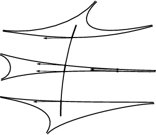
Figure 8.
Lemma 7.7.

Let kk be an arc in U^\widehat{U} that is tightly transverse to λ^\widehat{\lambda}, and let dd be a component of k−λ^k-\widehat{\lambda} that contains none of the two endpoints of kk. Then,

∫dωa=log⁡‖va​(ud−)‖ud−‖Σgd+​gd−​(va​(ud−))‖ud+\int_{d}\omega_{a}=\log\frac{\|v_{a}(u_{d}^{-})\|_{u_{d}^{-}}}{\bigl\|\Sigma_{g_{d}^{+}g_{d}^{-}}\bigl(v_{a}(u_{d}^{-})\bigr)\bigr\|_{u_{d}^{+}}}

for any non-zero vector va​(ud−)v_{a}(u_{d}^{-}) in the line L~a​(ud−)\widetilde{L}_{a}(u_{d}^{-}).

Proof.

The two leaves gd+g_{d}^{+} and gd−g_{d}^{-} are asymptotic. We can therefore find points yd+∈gd+y_{d}^{+}\in g_{d}^{+} and yd−∈gd−y_{d}^{-}\in g_{d}^{-} which are arbitrarily close to each other. Let wd±w_{d}^{\pm} be the element of the unit tangent bundle T1​S~T^{1}\widetilde{S} determined by the tangent of the oriented geodesic gd±g_{d}^{\pm} at the point yd±y_{d}^{\pm}. See Figure 8. We can then deform dd to an arc consisting of the arc from xd−x_{d}^{-} to yd−y_{d}^{-} in the leaf gd−g_{d}^{-}, followed by a short arc from yd−y_{d}^{-} to yd+y_{d}^{+}, and completed by the arc from yd+y_{d}^{+} to xd+x_{d}^{+} in gd+g_{d}^{+}. Then, by definition of the form ωa\omega_{a},

∫dωa\displaystyle\int_{d}\omega_{a} =∫xd−yd−ωa+∫yd−yd+ωa+∫yd+xd+ωa\displaystyle=\int_{x_{d}^{-}}^{y_{d}^{-}}\omega_{a}+\int_{y_{d}^{-}}^{y_{d}^{+}}\omega_{a}+\int_{y_{d}^{+}}^{x_{d}^{+}}\omega_{a}
=log⁡‖va​(ud−)‖ud−‖va​(ud−)‖wd−+∫yd−yd+ωa+log⁡‖va​(ud+)‖wd+‖va​(ud+)‖ud+\displaystyle=\log\frac{\|v_{a}(u_{d}^{-})\|_{u_{d}^{-}}}{\|v_{a}(u_{d}^{-})\|_{w_{d}^{-}}}+\int_{y_{d}^{-}}^{y_{d}^{+}}\omega_{a}+\log\frac{\|v_{a}(u_{d}^{+})\|_{w_{d}^{+}}}{\|v_{a}(u_{d}^{+})\|_{u_{d}^{+}}}

for arbitrary non-zero vectors va​(ud+)∈L~a​(ud+)v_{a}(u_{d}^{+})\in\widetilde{L}_{a}(u_{d}^{+}) and va​(ud−)∈L~a​(ud−)v_{a}(u_{d}^{-})\in\widetilde{L}_{a}(u_{d}^{-}). In particular, we can choose va​(ud+)=Σgd+​gd−​(va​(ud−))v_{a}(u_{d}^{+})=\Sigma_{g_{d}^{+}g_{d}^{-}}\bigl(v_{a}(u_{d}^{-})\bigr), in which case

∫dωa=log⁡‖va​(ud−)‖ud−‖Σgd+​gd−​(va​(ud−))‖ud+−log⁡‖va​(ud−)‖wd−‖Σgd+​gd−​(va​(ud−))‖wd++∫yd−yd+ωa.\int_{d}\omega_{a}=\log\frac{\|v_{a}(u_{d}^{-})\|_{u_{d}^{-}}}{\bigl\|\Sigma_{g_{d}^{+}g_{d}^{-}}\bigl(v_{a}(u_{d}^{-})\bigr)\bigr\|_{u_{d}^{+}}}-\log\frac{\|v_{a}(u_{d}^{-})\|_{w_{d}^{-}}}{\bigl\|\Sigma_{g_{d}^{+}g_{d}^{-}}\bigl(v_{a}(u_{d}^{-})\bigr)\bigr\|_{w_{d}^{+}}}+\int_{y_{d}^{-}}^{y_{d}^{+}}\omega_{a}.

Now, we let the points yd+y_{d}^{+} and yd−y_{d}^{-} tend to the common endpoint of gd+g_{d}^{+} and gd−g_{d}^{-} in such a way that the distance from yd+y_{d}^{+} to yd−y_{d}^{-} tends to 0. Looking at the projections to SS, the integral ∫yd−yd+ωa\int_{y_{d}^{-}}^{y_{d}^{+}}\omega_{a} tends to 0, while the quotient ‖va​(ud−)‖wd−‖Σgd+​gd−​(va​(ud−))‖wd+\frac{\|v_{a}(u_{d}^{-})\|_{w_{d}^{-}}}{\bigl\|\Sigma_{g_{d}^{+}g_{d}^{-}}\bigl(v_{a}(u_{d}^{-})\bigr)\bigr\|_{w_{d}^{+}}} tends to 1 (compare Lemma 5.2 and use the ρ\rho–equivariance of the riemannian metric ∥⁣∥\|\ \|). It follows that

∫dωa=log⁡‖va​(ud−)‖ud−‖Σgd+​gd−​(va​(ud−))‖ud+\int_{d}\omega_{a}=\log\frac{\|v_{a}(u_{d}^{-})\|_{u_{d}^{-}}}{\bigl\|\Sigma_{g_{d}^{+}g_{d}^{-}}\bigl(v_{a}(u_{d}^{-})\bigr)\bigr\|_{u_{d}^{+}}}

for any non-zero vector va​(ud−)∈L~a​(ud−)v_{a}(u_{d}^{-})\in\widetilde{L}_{a}(u_{d}^{-}). ∎

We will now choose preferred vectors va​(ud−)∈L~a​(ud−)v_{a}(u_{d}^{-})\in\widetilde{L}_{a}(u_{d}^{-}).

Let d+d^{+} and d−d^{-} be the components of k~−λ~\widetilde{k}-\widetilde{\lambda} that contain the positive and negative endpoints of k~\widetilde{k}, respectively. In particular, their endpoints xd+−x_{d^{+}}^{-} and xd−+x_{d^{-}}^{+} are the points of k~∩λ~\widetilde{k}\cap\widetilde{\lambda} that are closest to the positive and negative endpoints in k~\widetilde{k}, respectively. As usual, let ud±∓∈T1​S~u_{d^{\pm}}^{\mp}\in T^{1}\widetilde{S} be defined by the vector tangent to the (oriented) leaf gd±∓g_{d^{\pm}}^{\mp} of λ~\widetilde{\lambda} passing through xd±∓x_{d^{\pm}}^{\mp}. See Figure 8.

The flag map ℱρ:∂∞S~→Flag⁡(ℝn)\mathcal{F}_{\rho}\colon\partial_{\infty}\widetilde{S}\to\mathrm{Flag}(\mathbb{R}^{n}) associates several lines of ℝn\mathbb{R}^{n} to the vector ud+−∈T1​S~u_{d^{+}}^{-}\in T^{1}\widetilde{S}. This includes the nn lines L~a​(ud+−)=ℱρ​(x)(a)∩ℱρ​(y)(n−a+1)\widetilde{L}_{a}(u_{d^{+}}^{-})=\mathcal{F}_{\rho}(x)^{(a)}\cap\mathcal{F}_{\rho}(y)^{(n-a+1)} of §3.1, defined by the flags ℱρ​(x)\mathcal{F}_{\rho}(x) and ℱρ​(y)\mathcal{F}_{\rho}(y) respectively associated to the positive endpoint xx and the negative endpoint yy of the leaf gd+−g_{d^{+}}^{-}. We can also consider the line ℱρ​(z)(1)\mathcal{F}_{\rho}(z)^{(1)} of the flag ℱρ​(z)\mathcal{F}_{\rho}(z) associated to the third vertex zz of the triangle component of S~−λ~\widetilde{S}-\widetilde{\lambda} that contains d+d^{+}. Pick a non-trivial vector v⁡(ud+−)v(u_{d^{+}}^{-}) in this line ℱρ​(z)(1)\mathcal{F}_{\rho}(z)^{(1)}, and let va​(ud+−)∈L~a​(ud+−)v_{a}(u_{d^{+}}^{-})\in\widetilde{L}_{a}(u_{d^{+}}^{-}) be the projection of v⁡(ud+−)v(u_{d^{+}}^{-}) parallel to the L~b​(ud+−)\widetilde{L}_{b}(u_{d^{+}}^{-}) with b≠ab\neq a.

In particular, considering the riemannian metric ∥⁣∥\|\ \|, the quantity ‖va​(ud+−)‖ud+−‖va+1​(ud+−)‖ud+−\frac{\|v_{a}(u_{d^{+}}^{-})\|_{u_{d^{+}}^{-}}}{\|v_{a+1}(u_{d^{+}}^{-})\|_{u_{d^{+}}^{-}}} is independent of the choice of the vector v⁡(ud+−)∈ℱρ​(z)(1)v(u_{d^{+}}^{-})\in\mathcal{F}_{\rho}(z)^{(1)}. Note that this ratio is finite and positive by genericity of the flag triple (ℱρ​(x),ℱρ​(y),ℱρ​(z))\bigl(\mathcal{F}_{\rho}(x),\mathcal{F}_{\rho}(y),\mathcal{F}_{\rho}(z)\bigr).

We can introduce similar definitions at the point xd−+x_{d^{-}}^{+} of k~∩λ~\widetilde{k}\cap\widetilde{\lambda} that is closest to the negative endpoint of k~\widetilde{k}. Considering the triangle component of S~−λ~\widetilde{S}-\widetilde{\lambda} that contains the negative endpoint of k~\widetilde{k}, this leads to a well-defined positive ratio ‖va​(ud−+)‖ud−+‖va+1​(ud−+)‖ud−+\frac{\|v_{a}(u_{d^{-}}^{+})\|_{u_{d^{-}}^{+}}}{\|v_{a+1}(u_{d^{-}}^{+})\|_{u_{d^{-}}^{+}}}.

Lemma 7.8.

Let kk be an arc in U^\widehat{U} that is tightly transverse to λ^\widehat{\lambda}. Then, for the above definitions,

σaρ​(k)=∫k−d+∪d−(ωa−ωa+1)+log⁡‖va​(ud+−)‖ud+−‖va+1​(ud+−)‖ud+−−log⁡‖va​(ud−+)‖ud−+‖va+1​(ud−+)‖ud−+.\sigma_{a}^{\rho}(k)=\int_{k-d^{+}\cup d^{-}}(\omega_{a}-\omega_{a+1})+\log\frac{\|v_{a}(u_{d^{+}}^{-})\|_{u_{d^{+}}^{-}}}{\|v_{a+1}(u_{d^{+}}^{-})\|_{u_{d^{+}}^{-}}}-\log\frac{\|v_{a}(u_{d^{-}}^{+})\|_{u_{d^{-}}^{+}}}{\|v_{a+1}(u_{d^{-}}^{+})\|_{u_{d^{-}}^{+}}}.

Note that the notation is ambiguous in the special case where ud+−=ud−+u_{d^{+}}^{-}=u_{d^{-}}^{+}, which occurs when the arc kk crosses λ^\widehat{\lambda} in only one point. We will leave to the reader the easy task of lifting the ambiguity in this case.

Proof.

By a well-known result of Birman-Series [BS85], the intersection k~∩λ~\widetilde{k}\cap\widetilde{\lambda} has Hausdorff dimension 0. Since the topological closed 1–form ω\omega is Hölder continuous, if follows that

∫k−d+∪d−ωa=∑d∫dωa\int_{k-d^{+}\cup d^{-}}\omega_{a}=\sum_{d}\int_{d}\omega_{a}

where the sum is over all components dd of k~−λ~\widetilde{k}-\widetilde{\lambda} that are different from d+d^{+} and d−d^{-}. (The critical property is that the image of a set of Hausdorff dimension 0 under a Hölder continuous function has Hausdorff dimension 0, and in particular has Lebesgue measure 0 in ℝ\mathbb{R}.)

We now apply Lemma 7.7 while choosing va​(ud−)=Σgd−​gd−+​(va​(ud−+))∈La​(ud−)v_{a}(u_{d}^{-})=\Sigma_{g_{d}^{-}g_{d^{-}}^{+}}\bigl(v_{a}(u_{d^{-}}^{+})\bigr)\in L_{a}(u_{d}^{-}), where va​(ud−+)∈L~a​(ud−+)v_{a}(u_{d^{-}}^{+})\in\widetilde{L}_{a}(u_{d^{-}}^{+}) is determined as above by the vertices of the triangle component of S~−λ~\widetilde{S}-\widetilde{\lambda} that contains d+d^{+}. Then,

∫k−d+∪d−ωa=∑dlog⁡‖Σgd−​gd−+​(va​(ud−+))‖ud−‖Σgd+​gd−+​(va​(ud−+))‖ud+\int_{k-d^{+}\cup d^{-}}\omega_{a}=\sum_{d}\log\frac{\bigl\|\Sigma_{g_{d}^{-}g_{d^{-}}^{+}}\bigl(v_{a}(u_{d^{-}}^{+})\bigr)\bigr\|_{u_{d}^{-}}}{\bigl\|\Sigma_{g_{d}^{+}g_{d^{-}}^{+}}\bigl(v_{a}(u_{d^{-}}^{+})\bigr)\bigr\|_{u_{d}^{+}}}

by observing that

Σgd+​gd−​(va​(ud−))=Σgd+​gd−∘Σgd−​gd−+​(va​(ud−+))=Σgd+​gd−+​(va​(ud−+)).\Sigma_{g_{d}^{+}g_{d}^{-}}\bigl(v_{a}(u_{d}^{-})\bigr)=\Sigma_{g_{d}^{+}g_{d}^{-}}\circ\Sigma_{g_{d}^{-}g_{d^{-}}^{+}}\bigl(v_{a}(u_{d^{-}}^{+})\bigr)=\Sigma_{g_{d}^{+}g_{d^{-}}^{+}}\bigl(v_{a}(u_{d^{-}}^{+})\bigr).

If gxg_{x} denotes the oriented leaf of λ~\widetilde{\lambda} passing through x∈k~∩λ~x\in\widetilde{k}\cap\widetilde{\lambda} and if ux∈T1​S~u_{x}\in T^{1}\widetilde{S} is the unit vector tangent to gxg_{x} at xx, the map x↦‖Σgx​gd−+​(va​(ud−+))‖uxx\mapsto\bigl\|\Sigma_{g_{x}g_{d^{-}}^{+}}\bigl(v_{a}(u_{d^{-}}^{+})\bigr)\bigr\|_{u_{x}} is Hölder continuous, because gxg_{x} depends Lipshitz continuously on xx by [CEG87, §5.2.6]), and because the slithering map Σg​gd−+\Sigma_{gg_{d^{-}}^{+}} is a Hölder continuous function of the leaf gg by Proposition 5.1. Using again the fact that k~∩λ~\widetilde{k}\cap\widetilde{\lambda} has Hausdorff dimension 0, it follows that

∫k−d+∪d−ωa=∑dlog⁡‖Σgd−​gd−+​(va​(ud−+))‖ud−‖Σgd+​gd−+​(va​(ud−+))‖ud+=log⁡‖va​(ud−+)‖ud−+‖Σgd+−​gd−+​(va​(ud−+))‖ud+−.\int_{k-d^{+}\cup d^{-}}\omega_{a}=\sum_{d}\log\frac{\bigl\|\Sigma_{g_{d}^{-}g_{d^{-}}^{+}}\bigl(v_{a}(u_{d^{-}}^{+})\bigr)\bigr\|_{u_{d}^{-}}}{\bigl\|\Sigma_{g_{d}^{+}g_{d^{-}}^{+}}\bigl(v_{a}(u_{d^{-}}^{+})\bigr)\bigr\|_{u_{d}^{+}}}=\log\frac{\|v_{a}(u_{d^{-}}^{+})\|_{u_{d^{-}}^{+}}}{\bigl\|\Sigma_{g_{d^{+}}^{-}g_{d^{-}}^{+}}\bigl(v_{a}(u_{d^{-}}^{+})\bigr)\bigr\|_{u_{d^{+}}^{-}}}.

By construction, the slithering map Σgd+−​gd−+\Sigma_{g_{d^{+}}^{-}g_{d^{-}}^{+}} sends L~a​(ud−+)\widetilde{L}_{a}(u_{d^{-}}^{+}) to L~a​(ud+−)\widetilde{L}_{a}(u_{d^{+}}^{-}). In particular, there exists a non-zero number μa\mu_{a} such that Σgd+−​gd−+​(va​(ud−+))=μa​va​(ud+−)\Sigma_{g_{d^{+}}^{-}g_{d^{-}}^{+}}\bigl(v_{a}(u_{d^{-}}^{+})\bigr)=\mu_{a}v_{a}(u_{d^{+}}^{-}). Then,

∫k−d+∪d−(ωa−ωa+1)\displaystyle\int_{k-d^{+}\cup d^{-}}(\omega_{a}-\omega_{a+1}) =log⁡‖va​(ud−+)‖ud−+‖va+1​(ud−+)‖ud−+−log⁡‖va​(ud+−)‖ud+−‖va+1​(ud+−)‖ud+−−log⁡|μaμa+1|\displaystyle=\log\frac{\|v_{a}(u_{d^{-}}^{+})\|_{u_{d^{-}}^{+}}}{\|v_{a+1}(u_{d^{-}}^{+})\|_{u_{d^{-}}^{+}}}-\log\frac{\|v_{a}(u_{d^{+}}^{-})\|_{u_{d^{+}}^{-}}}{\|v_{a+1}(u_{d^{+}}^{-})\|_{u_{d^{+}}^{-}}}-\log\left|\frac{\mu_{a}}{\mu_{a+1}}\right|
=log⁡‖va​(ud−+)‖ud−+‖va+1​(ud−+)‖ud−+−log⁡‖va​(ud+−)‖ud+−‖va+1​(ud+−)‖ud+−+σaρ​(k)\displaystyle=\log\frac{\|v_{a}(u_{d^{-}}^{+})\|_{u_{d^{-}}^{+}}}{\|v_{a+1}(u_{d^{-}}^{+})\|_{u_{d^{-}}^{+}}}-\log\frac{\|v_{a}(u_{d^{+}}^{-})\|_{u_{d^{+}}^{-}}}{\|v_{a+1}(u_{d^{+}}^{-})\|_{u_{d^{+}}^{-}}}+\sigma_{a}^{\rho}(k)

by definition of the shear parameter σaρ​(k)\sigma_{a}^{\rho}(k) (use Lemma 1.6). ∎

Lemma 7.9.

For every homology class [α]∈H1​(U^,ℝ)[\alpha]\in H_{1}(\widehat{U};\mathbb{R}),

⟨[ωa]−[ωa+1],[α]⟩=[α]⋅[σaρ].\bigl\langle[\omega_{a}]-[\omega_{a+1}],[\alpha]\bigr\rangle=[\alpha]\cdot[\sigma_{a}^{\rho}].
Proof.

We already observed, in the proof of Proposition 4.5, that H1​(U^,∂hU^,ℝ)H_{1}(\widehat{U},\partial_{\mathrm{h}}\widehat{U};\mathbb{R}) admits a basis where each element is represented by a generic tie of U^\widehat{U}. We can therefore write the image [α]∈H1​(U^,∂hU^,ℝ)[\alpha]\in H_{1}(\widehat{U},\partial_{\mathrm{h}}\widehat{U};\mathbb{R}) as a linear combination [α]=∑iμi​[ki][\alpha]=\sum_{i}\mu_{i}[k_{i}] of classes represented by generic ties kik_{i}, with coefficients μi∈ℝ\mu_{i}\in\mathbb{R}.

Recall that the ties of U^\widehat{U} are oriented to the right for the canonical orientation of the leaves of λ^\widehat{\lambda}. In particular, the components of the horizontal boundary ∂hU^\partial_{\mathrm{h}}\widehat{U} are of two types: those components where the orientation of the ties point outside of U^\widehat{U}, and those where it points inside. Also, because of this orientation convention,

[α]⋅[σaρ]=∑iμi​[ki]⋅[σaρ]=∑iμi​σaρ​(ki)[\alpha]\cdot[\sigma_{a}^{\rho}]=\sum_{i}\mu_{i}\,[k_{i}]\cdot[\sigma_{a}^{\rho}]=\sum_{i}\mu_{i}\,\sigma_{a}^{\rho}(k_{i})

by definition of the homology class [σaρ]∈H1​(U^,∂vU^,ℝ)[\sigma_{a}^{\rho}]\in H_{1}(\widehat{U},\partial_{\mathrm{v}}\widehat{U};\mathbb{R}) associated to the relative tangent cycle σaρ∈𝒞⁡(λ^,slits,ℝ)\sigma_{a}^{\rho}\in\mathcal{C}(\widehat{\lambda},\mathrm{slits};\mathbb{R}) by Proposition 4.5.

We now modify each arc kik_{i} by a homotopy respecting λ^\widehat{\lambda} and ∂hU^\partial_{\mathrm{h}}\widehat{U} to obtain an arc ki′k_{i}^{\prime} such that the following holds: for every component CC of the horizontal boundary ∂hU^\partial_{\mathrm{h}}\widehat{U}, there is an arc kC⊂U^k_{C}\subset\widehat{U} such that, for every arc ki′k_{i}^{\prime} with an endpoint in CC, the component of ki′−λ^k_{i}^{\prime}-\widehat{\lambda} containing this endpoint is equal to kCk_{C}. The only case where this regrouping of arcs near the horizontal boundary requires some care is when the original tie kik_{i} meets λ^\widehat{\lambda} in one point; in this special situation, one needs to first choose the relevant arcs kCk_{C} so that ki′=kik_{i}^{\prime}=k_{i}, and then modify the other kjk_{j} accordingly.

Now, by Lemma 7.8,

∑iμi​σaρ​(ki′)\displaystyle\sum_{i}\mu_{i}\,\sigma_{a}^{\rho}(k_{i}^{\prime}) =∑iμi​∫ki′(ωa−ωa+1)\displaystyle=\sum_{i}\mu_{i}\int_{k_{i}^{\prime}}(\omega_{a}-\omega_{a+1})
−∑iμi∫di+(ωa−ωa+1)−∑iμi∫di−(ωa−ωa+1)\displaystyle\qquad-\sum_{i}\mu_{i}\int_{d_{i}^{+}}(\omega_{a}-\omega_{a+1})-\sum_{i}\mu_{i}\int_{d_{i}^{-}}(\omega_{a}-\omega_{a+1})
+∑iμilog‖va​(udi+−)‖udi+−‖va+1​(udi+−)‖udi+−−∑iμilog‖va​(udi−+)‖udi−+‖va+1​(udi−+)‖udi−+\displaystyle\qquad+\sum_{i}\mu_{i}\log\frac{\|v_{a}(u_{d_{i}^{+}}^{-})\|_{u_{d_{i}^{+}}^{-}}}{\|v_{a+1}(u_{d_{i}^{+}}^{-})\|_{u_{d_{i}^{+}}^{-}}}-\sum_{i}\mu_{i}\log\frac{\|v_{a}(u_{d_{i}^{-}}^{+})\|_{u_{d_{i}^{-}}^{+}}}{\|v_{a+1}(u_{d_{i}^{-}}^{+})\|_{u_{d_{i}^{-}}^{+}}}

where di+d_{i}^{+} and di−d_{i}^{-} are the components of ki′−λ^k_{i}^{\prime}-\widehat{\lambda} containing the positive and negative components of ki′k_{i}^{\prime}, respectively. In particular, each di±d_{i}^{\pm} is equal to one of the arcs kCk_{C} associated to the components CC of the horizontal boundary ∂hU^\partial_{\mathrm{h}}\widehat{U}.

The key observation is now that [α]=∑iμi​[ki]∈H1​(U^,∂hU^,ℝ)[\alpha]=\sum_{i}\mu_{i}[k_{i}]\in H_{1}(\widehat{U},\partial_{\mathrm{h}}\widehat{U};\mathbb{R}) comes from an element of H1​(U^,ℝ)H_{1}(\widehat{U};\mathbb{R}), and in particular has boundary 0. This implies that, for each component CC of ∂hU^\partial_{\mathrm{h}}\widehat{U} where the ties point outwards, the sum of the μi\mu_{i} such that kik_{i} has an endpoint in CC is equal to 0; equivalently, the μi\mu_{i} such that di+=kCd_{i}^{+}=k_{C} add up to 0. Similarly, for each component CC of ∂hU^\partial_{\mathrm{h}}\widehat{U} where the ties point inwards, the sum of the coefficients μi\mu_{i} such that di−=kCd_{i}^{-}=k_{C} is equal to 0.

This implies that most terms cancel out in the above sum, and that

∑iμi​σaρ​(ki′)=∑iμi​∫ki′(ωa−ωa+1)=⟨[ωa]−[ωa+1],[α]⟩.\sum_{i}\mu_{i}\sigma_{a}^{\rho}(k_{i}^{\prime})=\sum_{i}\mu_{i}\int_{k_{i}^{\prime}}(\omega_{a}-\omega_{a+1})=\bigl\langle[\omega_{a}]-[\omega_{a+1}],[\alpha]\bigr\rangle.

For the second equality note that, because the μi\mu_{i} for which the positive (resp. negative) endpoint of ki′k_{i}^{\prime} is in a given component CC of ∂hU^\partial_{\mathrm{h}}\widehat{U} add up to 0, the chain ∑iμi​ki′\sum_{i}\mu_{i}k_{i}^{\prime} is closed and represents the class [α]∈H1​(U^,ℝ)[\alpha]\in H_{1}(\widehat{U};\mathbb{R}).

This proves that

[α]⋅[σa]=∑iμi​σa​(ki)=∑iμi​σa​(ki′)=⟨[ωa]−[ωa+1],[α]⟩.∎[\alpha]\cdot[\sigma_{a}]=\sum_{i}\mu_{i}\sigma_{a}(k_{i})=\sum_{i}\mu_{i}\sigma_{a}(k_{i}^{\prime})=\bigl\langle[\omega_{a}]-[\omega_{a+1}],[\alpha]\bigr\rangle.\qed

The combination of Lemmas 7.6 and 7.9 completes the proof of Theorem 7.5. ∎

Corollary 7.10.

Let μ\mu be a non-trivial transverse measure for the orientation cover λ^\widehat{\lambda}, and let [μ]∈H1​(U^,ℝ)[\mu]\in H_{1}(\widehat{U};\mathbb{R}) be its associated homology class as in §4.3. Then,

[μ]⋅[σaρ]>0[\mu]\cdot[\sigma_{a}^{\rho}]>0

for each component σaρ∈𝒞⁡(λ^,slits,ℝ)≅H1​(U^,∂vU^,ℝ)\sigma_{a}^{\rho}\in\mathcal{C}(\widehat{\lambda},\mathrm{slits};\mathbb{R})\cong H_{1}(\widehat{U},\partial_{\mathrm{v}}\widehat{U};\mathbb{R}) of the shearing cycle σρ∈𝒞⁡(λ,slits,ℝ^n−1)\sigma^{\rho}\in\mathcal{C}(\lambda,\mathrm{slits};\widehat{\mathbb{R}}^{n-1}) of a Hichin character ρ∈Hitn​(S)\rho\in\mathrm{Hit}_{\mathrm{n}}(S).

Proof.

This is an immediate consequence of Theorem 7.5 and Proposition 7.4. ∎

8. Parametrizing Hitchin components

In §3 and §5.2, we associated certain invariants to a Hitchin character ρ∈Hitn​(S)\rho\in\mathrm{Hit}_{\mathrm{n}}(S).

The first type of invariants are the triangle invariants τa​b​cρ​(s)\tau_{abc}^{\rho}(s), defined as ss ranges over the slits of λ\lambda and aa, bb, c⩾1c\geqslant 1 range over all integers such that a+b+c=na+b+c=n. Noting that there are (n−1)​(n−2)2\frac{(n-1)(n-2)}{2} such triples (a,b,c)(a,b,c) and 12​(g−1)12(g-1) slits of S−λS-\lambda, we can combine all these invariants into a single map

Hitn​(S)→ℝ6​(g−1)​(n−1)​(n−2).\mathrm{Hit}_{\mathrm{n}}(S)\to\mathbb{R}^{6(g-1)(n-1)(n-2)}.

The second invariant is the shearing cycle σρ∈𝒞⁡(λ,slits,ℝ^n)\sigma^{\rho}\in\mathcal{C}(\lambda,\mathrm{slits};\widehat{\mathbb{R}}^{n}), which provides a map

Hitn​(S)→𝒞⁡(λ,slits,ℝ^n)≅ℝ18​(g−1)​(n−1).\mathrm{Hit}_{\mathrm{n}}(S)\to\mathcal{C}(\lambda,\mathrm{slits};\widehat{\mathbb{R}}^{n})\cong\mathbb{R}^{18(g-1)(n-1)}.

Combining these two maps, we define

Φ:Hitn​(S)→ℝ6​(g−1)​(n−1)​(n−2)×𝒞⁡(λ,slits,ℝ^n)≅ℝ6​(g−1)​(n+1)​(n−1),\Phi\colon\mathrm{Hit}_{\mathrm{n}}(S)\to\mathbb{R}^{6(g-1)(n-1)(n-2)}\times\mathcal{C}(\lambda,\mathrm{slits};\widehat{\mathbb{R}}^{n})\cong\mathbb{R}^{6(g-1)(n+1)(n-1)},

which sends each Hitchin character ρ∈Hitn​(S)\rho\in\mathrm{Hit}_{\mathrm{n}}(S) to its triangle invariants and its shearing cycle. We will show that Φ\Phi induces a homeomorphism between Hitn​(S)\mathrm{Hit}_{\mathrm{n}}(S) and an open convex polyhedral cone 𝒫\mathcal{P} contained in a linear subspace of ℝ6​(g−1)​(n+1)​(n−1)\mathbb{R}^{6(g-1)(n+1)(n-1)}.

Lemma 8.1.

The above map

Φ:Hitn​(S)→ℝ6​(g−1)​(n−1)​(n−2)×𝒞⁡(λ,slits,ℝ^n)\Phi\colon\mathrm{Hit}_{\mathrm{n}}(S)\to\mathbb{R}^{6(g-1)(n-1)(n-2)}\times\mathcal{C}(\lambda,\mathrm{slits};\widehat{\mathbb{R}}^{n})

is continuous.

Proof.

The key property is that the flag curve ℱρ:∂∞S~→Flag⁡(ℝn)\mathcal{F}_{\rho}\colon\partial_{\infty}\widetilde{S}\to\mathrm{Flag}(\mathbb{R}^{n}) depends continuously on the Hitchin homomorphism ρ:π1​(S)→PSLn​(ℝ)\rho\colon\pi_{1}(S)\to\mathrm{PSL_{n}(\mathbb{R})}, and is uniformly Hölder continuous as ρ\rho ranges over a compact subset of the space of homomorphisms π1​(S)→PSLn​(ℝ)\pi_{1}(S)\to\mathrm{PSL_{n}(\mathbb{R})}. These two properties follow from the application to the setup of §3.1 of the classical structural stability theorems for Anosov flows, and Hölder continuity properties for their stable and unstable foliations; see for instance [KH95, §18–19].

The continuity property immediately shows that the triangle invariants τa​b​cρ​(s)\tau_{abc}^{\rho}(s) depend continuously on ρ\rho.

The case of the shearing cycle σρ∈𝒞⁡(λ,slits,ℝ^n)\sigma^{\rho}\in\mathcal{C}(\lambda,\mathrm{slits};\widehat{\mathbb{R}}^{n}) requires an additional argument, because its construction relies on the slithering maps Σg​g′:ℝn→ℝn\Sigma_{gg^{\prime}}\colon\mathbb{R}^{n}\to\mathbb{R}^{n}. The uniform Hölder continuity property makes the estimates used in the construction of slithering maps in §5.1 uniform, and guarantees uniform convergence in this construction. It follows that, for any two leaves gg, g′g^{\prime} of λ~\widetilde{\lambda}, the slithering map Σg​g′\Sigma_{gg^{\prime}} depends continuously on ρ\rho. After this, the continuous dependence of the flag map ℱρ\mathcal{F}_{\rho} on ρ\rho is enough to prove that σρ\sigma^{\rho} depends continuously on ρ\rho. ∎

8.1. Constraints between invariants

There are clear constraints on the image of Φ\Phi. The first one is the following consequence of Lemma 1.1, which we have already encountered in Lemma 3.4.

Triangle Rotation Condition: If the spikes of the component TT of S−λS-\lambda are indexed as ss, s′s^{\prime}, s′′s^{\prime\prime} in counterclockwise order around TT, then

τa​b​cρ​(s)=τb​c​aρ​(s′)=τc​a​bρ​(s′′).\tau_{abc}^{\rho}(s)=\tau_{bca}^{\rho}(s^{\prime})=\tau_{cab}^{\rho}(s^{\prime\prime}).

The second constraint comes from the quasi-additivity property of the shearing cycle σρ\sigma^{\rho}. Recall that the lack of additivity of the aa–th component σaρ∈𝒞⁡(λ^,slits,ℝn−1)\sigma_{a}^{\rho}\in\mathcal{C}(\widehat{\lambda},\mathrm{slits};\mathbb{R}^{n-1}) of σρ∈𝒞⁡(λ,slits,ℝ^n−1)⊂𝒞⁡(λ^,slits,ℝn−1)\sigma^{\rho}\in\mathcal{C}(\lambda,\mathrm{slits};\widehat{\mathbb{R}}^{n-1})\subset\mathcal{C}(\widehat{\lambda},\mathrm{slits};\mathbb{R}^{n-1}) is measured by its boundary ∂σaρ\partial\sigma^{\rho}_{a}, which associates a number σaρ​(s^)∈ℝ\sigma^{\rho}_{a}(\widehat{s})\in\mathbb{R} to each spike s^\widehat{s} of the orientation cover λ^\widehat{\lambda} of the geodesic lamination λ\lambda. The spikes s^\widehat{s} can be positive of negative, according to whether the canonical orientation of the leaves of λ^\widehat{\lambda} orients the two leaves that are adjacent to s^\widehat{s} towards s^\widehat{s} or away from s^\widehat{s}.

The following constraint comes from the computation of ∂σaρ\partial\sigma_{a}^{\rho} provided by Lemmas 5.14 and 5.13.

Shearing Cycle Boundary Condition: For every positive slit s+s^{+} of λ^\widehat{\lambda} projecting to a slit ss of λ\lambda,

∂σaρ​(s+)=∑b+c=n−aτa​b​cρ​(s).\partial\sigma^{\rho}_{a}(s^{+})=\sum_{b+c=n-a}\tau^{\rho}_{abc}(s).

Note that this property for positive slits, combined with the equivariance property of σρ∈𝒞⁡(λ,slits,ℝ^n−1)⊂𝒞⁡(λ^,slits,ℝn−1)\sigma^{\rho}\in\mathcal{C}(\lambda,\mathrm{slits};\widehat{\mathbb{R}}^{n-1})\subset\mathcal{C}(\widehat{\lambda},\mathrm{slits};\mathbb{R}^{n-1}) with respect to the covering involution of the cover λ^→λ\widehat{\lambda}\to\lambda, determines ∂σaρ\partial\sigma^{\rho}_{a} on negative slits. More precisely,

∂σaρ(s−)=−∑b+c=aτ(n−a)​b​cρ(s)\partial\sigma^{\rho}_{a}(s^{-})=-\sum_{b+c=a}\tau^{\rho}_{(n-a)bc}(s)

for every negative slit s−s^{-} of λ^\widehat{\lambda} projecting to a slit ss of λ\lambda.

The last condition is provided by Corollary 7.10.

Positive Intersection Condition:

[μ]⋅[σaρ]>0[\mu]\cdot[\sigma^{\rho}_{a}]>0

for every transverse measure μ\mu for λ^\widehat{\lambda}, where [μ]∈H1​(U^,ℝ)[\mu]\in H_{1}(\widehat{U};\mathbb{R}) and [σaρ]∈H1​(U^,∂vU^,ℝ)[\sigma_{a}^{\rho}]\in H_{1}(\widehat{U},\partial_{\mathrm{v}}\widehat{U};\mathbb{R}) are the homology classes respectively defined by μ∈𝒞⁡(λ^,ℝ)\mu\in\mathcal{C}(\widehat{\lambda};\mathbb{R}) and by the aa–th component σaρ∈𝒞⁡(λ^,slits,ℝ)\sigma_{a}^{\rho}\in\mathcal{C}(\widehat{\lambda},\mathrm{slits};\mathbb{R}) of the shearing cycle σρ∈𝒞⁡(λ,ℝ^n−1)⊂𝒞⁡(λ^,slits,ℝn−1)\sigma^{\rho}\in\mathcal{C}(\lambda;\widehat{\mathbb{R}}^{n-1})\subset\mathcal{C}(\widehat{\lambda},\mathrm{slits};\mathbb{R}^{n-1}), and where ⋅\cdot denotes the algebraic intersection in U^\widehat{U}.

Let 𝒫\mathcal{P} be the set of pairs (τ,σ)(\tau,\sigma) such that

  1. (1)

    τ\tau is a function associating a number τa​b​c​(s)∈ℝ\tau_{abc}(s)\in\mathbb{R} to each triple of integers aa, bb, c⩾1c\geqslant 1 with a+b+c=na+b+c=n, and to each slit ss of λ\lambda;

  2. (2)

    σ∈𝒞⁡(λ,slits,ℝ^n−1)\sigma\in\mathcal{C}(\lambda,\mathrm{slits};\widehat{\mathbb{R}}^{n-1}) is a tangent cycle for λ\lambda valued in the coefficient bundle ℝ^n−1\widehat{\mathbb{R}}^{n-1} and relative to the slits of λ\lambda; in particular, σ\sigma is defined by n−1n-1 relative tangent cycles σa∈𝒞⁡(λ^,slits,ℝ)\sigma_{a}\in\mathcal{C}(\widehat{\lambda},\mathrm{slits};\mathbb{R});

  3. (3)

    τ\tau and σ\sigma satisfy the above Triangle Rotation Condition, Shearing Cycle Boundary Condition and Positive Intersection Condition.

We will call a function τ∈ℝ6​(g−1)​(n−1)​(n−2)\tau\in\mathbb{R}^{6(g-1)(n-1)(n-2)} as in (1) a triangle data function. It is rotation invariant when it satisfies the Triangle Rotation Condition.

Proposition 8.2.

The space 𝒫\mathcal{P} is an open convex polyhedral cone in a 2​(g−1)​(n2−1)2(g-1)(n^{2}-1)–dimensional subspace of ℝ6​(g−1)​(n−1)​(n−2)×𝒞⁡(λ,slits,ℝ^n−1)\mathbb{R}^{6(g-1)(n-1)(n-2)}\times\mathcal{C}(\lambda,\mathrm{slits};\widehat{\mathbb{R}}^{n-1}).

Proof.

The transverse measures for the geodesic lamination λ^\widehat{\lambda} form a positive cone over a finite-dimensional simplex [Kat73, Pap86]. It therefore suffices to check the Positive Intersection Condition on the vertices of this simplex (corresponding to ergodic measures). This reduces the Positive Intersection Condition to finitely many linear inequalities. As a consequence, 𝒫\mathcal{P} is an open convex polyhedral cone in the linear subspace of ℝ6​(g−1)​(n−1)​(n−2)×𝒞⁡(λ,slits,ℝ^n)\mathbb{R}^{6(g-1)(n-1)(n-2)}\times\mathcal{C}(\lambda,\mathrm{slits};\widehat{\mathbb{R}}^{n}) defined by the Triangle Rotation Condition and the Shearing Cycle Boundary Condition. We need to compute its dimension, which will require a few lemmas.

The Triangle Rotation Condition divides the dimension of the space of triangle data functions by 33, in the sense that the space of rotation invariant triangle data functions τ∈ℝ6​(g−1)​(n−1)​(n−2)\tau\in\mathbb{R}^{6(g-1)(n-1)(n-2)} is isomorphic to ℝ2​(g−1)​(n−1)​(n−2)\mathbb{R}^{2(g-1)(n-1)(n-2)}. Indeed, if we pick a spike sjs_{j} for each triangle component TjT_{j} of S−λS-\lambda, such a rotation invariant τ\tau is completely determined by the 2​(g−1)​(n−1)​(n−2)2(g-1)(n-1)(n-2) numbers τa​b​c​(sj)\tau_{abc}(s_{j}). We will use this observation to denote by ℝ2​(g−1)​(n−1)​(n−2)\mathbb{R}^{2(g-1)(n-1)(n-2)} the space of all rotation invariant triangle data functions τ\tau.

Consider the linear subspace ℒ⊂ℝ2​(g−1)​(n−1)​(n−2)×𝒞⁡(λ,slits,ℝ^n−1)\mathcal{L}\subset\mathbb{R}^{2(g-1)(n-1)(n-2)}\times\mathcal{C}(\lambda,\mathrm{slits};\widehat{\mathbb{R}}^{n-1}) consisting of all pairs (τ,σ)(\tau,\sigma) where τ\tau is a rotation invariant triangle data function, where σ\sigma is a twisted tangent cycle for λ\lambda relative to its slits, and where τ\tau and σ\sigma satisfy the Shearing Cycle Boundary Condition.

To analyze ℒ\mathcal{L}, we introduce a new vector space 𝒞⁡(slits,ℝn−1)\mathcal{C}(\mathrm{slits};\mathbb{R}^{n-1}), consisting of all functions θ:{slits of ​λ}→ℝn−1\theta\colon\{\text{slits of }\lambda\}\to\mathbb{R}^{n-1}. For a=1a=1, 22, …, n−1n-1, we denote the aa–th component of such a θ∈𝒞⁡(slits,ℝn−1)\theta\in\mathcal{C}(\mathrm{slits};\mathbb{R}^{n-1}) by θa:{slits of ​λ}→ℝ\theta_{a}\colon\{\text{slits of }\lambda\}\to\mathbb{R}. The definition of the space ℒ\mathcal{L} can then be expressed in terms of two maps ∂:𝒞⁡(λ,slits,ℝ^n−1)→𝒞⁡(slits,ℝn−1)\partial\colon\mathcal{C}(\lambda,\mathrm{slits};\widehat{\mathbb{R}}^{n-1})\to\mathcal{C}(\mathrm{slits};\mathbb{R}^{n-1}) and Θ:ℝ2​(g−1)​(n−1)​(n−2)→𝒞⁡(slits,ℝn−1)\Theta\colon\mathbb{R}^{2(g-1)(n-1)(n-2)}\to\mathcal{C}(\mathrm{slits};\mathbb{R}^{n-1}).

The first map ∂:𝒞⁡(λ,slits,ℝ^n−1)→𝒞⁡(slits,ℝn−1)\partial\colon\mathcal{C}(\lambda,\mathrm{slits};\widehat{\mathbb{R}}^{n-1})\to\mathcal{C}(\mathrm{slits};\mathbb{R}^{n-1}) is the usual boundary map, and associates to a relative cycle σ∈𝒞⁡(λ,slits,ℝ^n−1)\sigma\in\mathcal{C}(\lambda,\mathrm{slits};\widehat{\mathbb{R}}^{n-1}) the restriction ∂σ:{positive slits of ​λ^}={slits of ​λ}→ℝn−1\partial\sigma\colon\{\text{positive slits of }\widehat{\lambda}\}=\{\text{slits of }\lambda\}\to\mathbb{R}^{n-1} of its boundary ∂σ\partial\sigma to positive slits of the orientation cover λ^\widehat{\lambda}. (Recall that this restriction completely determines ∂σ\partial\sigma by definition of twisted relative tangent cycles, as ∂σa(s−)=−∂σn−a(s+)\partial\sigma_{a}(s^{-})=-\partial\sigma_{n-a}(s^{+}) when the negative slit s−s^{-} of λ^\widehat{\lambda} projects to the same slit of λ\lambda as the positive slit s+s^{+}.)

The second map Θ:ℝ2​(g−1)​(n−1)​(n−2)→𝒞⁡(slits,ℝn−1)\Theta\colon\mathbb{R}^{2(g-1)(n-1)(n-2)}\to\mathcal{C}(\mathrm{slits};\mathbb{R}^{n-1}) associates to each rotation invariant triangle data function τ∈ℝ2​(g−1)​(n−1)​(n−2)\tau\in\mathbb{R}^{2(g-1)(n-1)(n-2)} the function θτ:{slits of ​λ}→ℝn−1\theta^{\tau}\colon\{\text{slits of }\lambda\}\to\mathbb{R}^{n-1} defined by the property that

θaτ​(s)=∑b+c=n−aτa​b​c​(s)∈ℝ\theta_{a}^{\tau}(s)=\sum_{b+c=n-a}\tau_{abc}(s)\in\mathbb{R}

for every slit ss of λ\lambda and every a=1a=1, 22, …, n−1n-1.

Then the subspace ℒ\mathcal{L} consists of all pairs (τ,σ)∈ℝ2​(g−1)​(n−1)​(n−2)×𝒞⁡(λ,slits,ℝ^n−1)(\tau,\sigma)\in\mathbb{R}^{2(g-1)(n-1)(n-2)}\times\mathcal{C}(\lambda,\mathrm{slits};\widehat{\mathbb{R}}^{n-1}) such that ∂σ=Θ⁡(τ)\partial\sigma=\Theta(\tau) in 𝒞⁡(slits,ℝn−1)\mathcal{C}(\mathrm{slits};\mathbb{R}^{n-1}).

Lemma 8.3.

The image of ∂:𝒞⁡(λ,slits,ℝ^n−1)→𝒞⁡(slits,ℝn−1)\partial\colon\mathcal{C}(\lambda,\mathrm{slits};\widehat{\mathbb{R}}^{n-1})\to\mathcal{C}(\mathrm{slits};\mathbb{R}^{n-1}) consists of all θ∈𝒞⁡(slits,ℝn−1)\theta\in\mathcal{C}(\mathrm{slits};\mathbb{R}^{n-1}) such that

∑s​ slit of ​λθa​(s)=∑s​ slit of ​λθn−a​(s)\sum_{s\text{ slit of }\lambda}\theta_{a}(s)=\sum_{s\text{ slit of }\lambda}\theta_{n-a}(s)

for every a=1a=1, 22, …, n−1n-1. This image has codimension ⌊n−12⌋\lfloor\frac{n-1}{2}\rfloor in 𝒞⁡(slits,ℝn−1)≅ℝ12​(g−1)​(n−1)\mathcal{C}(\mathrm{slits};\mathbb{R}^{n-1})\cong\mathbb{R}^{12(g-1)(n-1)}.

Proof.

This is an immediate consequence of the homological interpretation of twisted relative tangent cycles in §4.6, and more precisely of the isomorphism 𝒞⁡(λ,slits,ℝ^n−1)≅H1​(U,∂vU,ℝ~n−1)\mathcal{C}(\lambda,\mathrm{slits};\widehat{\mathbb{R}}^{n-1})\cong H_{1}(U,\partial_{\mathrm{v}}U;\widetilde{\mathbb{R}}^{n-1}) constructed there.

This construction is well behaved with respect to the boundary maps ∂\partial in the following sense. There is a unique isomorphism 𝒞⁡(slits,ℝn−1)≅H0​(∂vU,ℝ~n−1)\mathcal{C}(\mathrm{slits};\mathbb{R}^{n-1})\cong H_{0}(\partial_{\mathrm{v}}U;\widetilde{\mathbb{R}}^{n-1}) defined as follows: this isomorphism associates to θ∈𝒞⁡(slits,ℝn−1)\theta\in\mathcal{C}(\mathrm{slits};\mathbb{R}^{n-1}) the element of H0​(∂vU,ℝ~n−1)⊂H0​(∂vU^,ℝn−1)H_{0}(\partial_{\mathrm{v}}U;\widetilde{\mathbb{R}}^{n-1})\subset H_{0}(\partial_{\mathrm{v}}\widehat{U};\mathbb{R}^{n-1}) that assigns to each component of ∂vU^\partial_{\mathrm{v}}\widehat{U} facing a positive slit s+s^{+} the multiplicity θ⁡(s)∈ℝn−1\theta(s)\in\mathbb{R}^{n-1} associated by θ\theta to the projection ss of s+s^{+} (and assigns multiplicity −θn−a​(s)-\theta_{n-a}(s) to the component of ∂vU^\partial_{\mathrm{v}}\widehat{U} facing a negative slit s−s^{-} projecting to ss). Then, for these isomorphisms 𝒞⁡(λ,slits,ℝ^n−1)≅H1​(U,∂vU,ℝ~n−1)\mathcal{C}(\lambda,\mathrm{slits};\widehat{\mathbb{R}}^{n-1})\cong H_{1}(U,\partial_{\mathrm{v}}U;\widetilde{\mathbb{R}}^{n-1}) and 𝒞⁡(slits,ℝn−1)≅H0​(∂vU,ℝ~n−1)\mathcal{C}(\mathrm{slits};\mathbb{R}^{n-1})\cong H_{0}(\partial_{\mathrm{v}}U;\widetilde{\mathbb{R}}^{n-1}), the boundary homomorphism ∂:𝒞⁡(λ,slits,ℝ^n−1)→𝒞⁡(slits,ℝn−1)\partial\colon\mathcal{C}(\lambda,\mathrm{slits};\widehat{\mathbb{R}}^{n-1})\to\mathcal{C}(\mathrm{slits};\mathbb{R}^{n-1}) corresponds to the homological boundary ∂:H1​(U,∂vU,ℝ~n−1)→H0​(∂vU,ℝ~n−1)\partial\colon H_{1}(U,\partial_{\mathrm{v}}U;\widetilde{\mathbb{R}}^{n-1})\to H_{0}(\partial_{\mathrm{v}}U;\widetilde{\mathbb{R}}^{n-1}).

Lemma 8.3 is then an immediate consequence of the long exact sequence

…→H1​(U,∂vU,ℝ~n−1)→H0​(∂vU,ℝ~n−1)→H0​(U,ℝ~n−1)→H0​(U,∂vU,ℝ~n−1),\dots\to H_{1}(U,\partial_{\mathrm{v}}U;\widetilde{\mathbb{R}}^{n-1})\to H_{0}(\partial_{\mathrm{v}}U;\widetilde{\mathbb{R}}^{n-1})\to H_{0}(U;\widetilde{\mathbb{R}}^{n-1})\to H_{0}(U,\partial_{\mathrm{v}}U;\widetilde{\mathbb{R}}^{n-1}),

using the properties that, because U^\widehat{U} is connected and ∂vU^\partial_{\mathrm{v}}\widehat{U} is non-empty, dimH0​(U,ℝ~n−1)=⌊n−12⌋\dim H_{0}(U;\widetilde{\mathbb{R}}^{n-1})=\lfloor\frac{n-1}{2}\rfloor and H0​(U,∂vU,ℝ~n−1)=0H_{0}(U,\partial_{\mathrm{v}}U;\widetilde{\mathbb{R}}^{n-1})=0. ∎

Lemma 8.4.

For n>3n>3, the image of Θ:ℝ2​(g−1)​(n−1)​(n−2)→𝒞⁡(slits,ℝn−1)\Theta\colon\mathbb{R}^{2(g-1)(n-1)(n-2)}\to\mathcal{C}(\mathrm{slits};\mathbb{R}^{n-1}) consists of all θ∈𝒞⁡(slits,ℝn−1)\theta\in\mathcal{C}(\mathrm{slits};\mathbb{R}^{n-1}) such that

θn−1​(s1)\displaystyle\theta_{n-1}(s_{1}) =0\displaystyle=0
and ​θ1​(s1)\displaystyle\text{and }\theta_{1}(s_{1}) =∑a=2n−2(a−1n−3−1)​θa​(s1)+∑a=2n−2a−1n−3​θa​(s2)+∑a=2n−2a−1n−3​θa​(s3)\displaystyle=\sum_{a=2}^{n-2}({\textstyle\frac{a-1}{n-3}}-1)\theta_{a}(s_{1})+\sum_{a=2}^{n-2}{\textstyle\frac{a-1}{n-3}}\,\theta_{a}(s_{2})+\sum_{a=2}^{n-2}{\textstyle\frac{a-1}{n-3}}\,\theta_{a}(s_{3})

whenever s1s_{1}, s2s_{2} and s3s_{3} are the three spikes of the same component TT of S−λS-\lambda. In particular, the image of Θ\Theta has dimension 12​(g−1)​(n−3)12(g-1)(n-3).

When n=3n=3, the image of Θ:ℝ4​(g−1)→𝒞⁡(slits,ℝ2)\Theta\colon\mathbb{R}^{4(g-1)}\to\mathcal{C}(\mathrm{slits};\mathbb{R}^{2}) consists of all θ∈𝒞⁡(slits,ℝ2)\theta\in\mathcal{C}(\mathrm{slits};\mathbb{R}^{2}) such that

θ2​(s1)\displaystyle\theta_{2}(s_{1}) =0\displaystyle=0
and ​θ1​(s1)\displaystyle\text{and }\theta_{1}(s_{1}) =θ1​(s2)=θ1​(s3)\displaystyle=\theta_{1}(s_{2})=\theta_{1}(s_{3})

whenever s1s_{1}, s2s_{2} and s3s_{3} are the three spikes of the same component TT of S−λS-\lambda. In particular, the image of Θ\Theta then has dimension 4​(g−1)4(g-1).

Proof.

By definition, if θτ=Θ⁡(τ)\theta^{\tau}=\Theta(\tau) for a rotation invariant function τ∈ℝ2​(g−1)​(n−1)​(n−2)\tau\in\mathbb{R}^{2(g-1)(n-1)(n-2)} , then θn−1τ​(s)=∑b+c=1τ(n−1)​b​c​(s)=0\theta_{n-1}^{\tau}(s)=\sum_{b+c=1}\tau_{(n-1)bc}(s)=0 for every slit ss since all indices bb, cc are supposed to be at least 1.

Less trivially, if n>3n>3 and if s1s_{1}, s2s_{2}, s3s_{3} are the three spikes of a same component TT of S−λS-\lambda, in this order counterclockwise around TT,

∑a=2n−2a−1n−3​θaτ​(s1)\displaystyle\sum_{a=2}^{n-2}{\textstyle\frac{a-1}{n-3}}\,\theta_{a}^{\tau}(s_{1}) +∑a=2n−2a−1n−3θaτ(s2)+∑a=2n−2a−1n−3θaτ(s3)\displaystyle+\sum_{a=2}^{n-2}{\textstyle\frac{a-1}{n-3}}\,\theta_{a}^{\tau}(s_{2})+\sum_{a=2}^{n-2}{\textstyle\frac{a-1}{n-3}}\,\theta_{a}^{\tau}(s_{3})
=∑a=1n−2a−1n−3​∑b+c=n−aτa​b​c​(s1)+∑a=1n−2a−1n−3​∑b+c=n−aτa​b​c​(s2)+∑a=1n−2a−1n−3​∑b+c=n−aτa​b​c​(s3)\displaystyle=\sum_{a=1}^{n-2}{\textstyle\frac{a-1}{n-3}}\kern-4.0pt\sum_{b+c=n-a}\kern-8.0pt\tau_{abc}(s_{1})+\sum_{a=1}^{n-2}{\textstyle\frac{a-1}{n-3}}\kern-4.0pt\sum_{b+c=n-a}\kern-8.0pt\tau_{abc}(s_{2})+\sum_{a=1}^{n-2}{\textstyle\frac{a-1}{n-3}}\kern-4.0pt\sum_{b+c=n-a}\kern-8.0pt\tau_{abc}(s_{3})
=∑a=1n−2a−1n−3​∑b+c=n−aτa​b​c​(s1)+∑b=1n−2b−1n−3​∑a+c=n−bτa​b​c​(s1)+∑c=1n−2c−1n−3​∑a+b=n−cτa​b​c​(s1)\displaystyle=\sum_{a=1}^{n-2}{\textstyle\frac{a-1}{n-3}}\kern-4.0pt\sum_{b+c=n-a}\kern-8.0pt\tau_{abc}(s_{1})+\sum_{b=1}^{n-2}{\textstyle\frac{b-1}{n-3}}\kern-4.0pt\sum_{a+c=n-b}\kern-8.0pt\tau_{abc}(s_{1})+\sum_{c=1}^{n-2}{\textstyle\frac{c-1}{n-3}}\kern-4.0pt\sum_{a+b=n-c}\kern-8.0pt\tau_{abc}(s_{1})
=∑a,b,c(a−1n−3+b−1n−3+c−1n−3)​τa​b​c​(s1)=∑a,b,cτa​b​c​(s1)=∑a=1n−1θaτ​(s1)\displaystyle=\sum_{a,b,c}\bigl({\textstyle\frac{a-1}{n-3}}+{\textstyle\frac{b-1}{n-3}}+{\textstyle\frac{c-1}{n-3}}\bigr)\tau_{abc}(s_{1})=\sum_{a,b,c}\tau_{abc}(s_{1})=\sum_{a=1}^{n-1}\theta_{a}^{\tau}(s_{1})

where the second equality uses the rotation invariance of τ\tau. It follows that

θ1τ​(s1)=∑a=2n−2(a−1n−3−1)​θaτ​(s1)+∑a=2n−2a−1n−3​θaτ​(s2)+∑a=2n−2a−1n−3​θaτ​(s3).\theta_{1}^{\tau}(s_{1})=\sum_{a=2}^{n-2}\bigl({\textstyle\frac{a-1}{n-3}}-1)\theta_{a}^{\tau}(s_{1})+\sum_{a=2}^{n-2}{\textstyle\frac{a-1}{n-3}}\,\theta_{a}^{\tau}(s_{2})+\sum_{a=2}^{n-2}{\textstyle\frac{a-1}{n-3}}\,\theta_{a}^{\tau}(s_{3}).

As a consequence, any function θ=Θ⁡(τ)\theta=\Theta(\tau) in the image of Θ\Theta satisfies the relations of Lemma 8.4.

Conversely, as aa ranges from 22 to n−2n-2 and ss ranges over all slits of λ\lambda, the functions τ↦θaτ​(s)\tau\mapsto\theta_{a}^{\tau}(s) are linearly independent over the space ℝ2​(g−1)​(n−1)​(n−2)\mathbb{R}^{2(g-1)(n-1)(n-2)} of rotation invariant triangle data functions τ\tau. Indeed, this follows from a simple computation focusing on the coefficients of the terms τ1​b​c​(s)\tau_{1bc}(s) and τ2​b​c​(s)\tau_{2bc}(s) in any linear relation between these functions.

The dimension computation then follows from the fact that λ\lambda has 12​(g−1)12(g-1) slits. This completes the proof of Lemma 8.4 in the case considered, when n>3n>3.

The proof is much simpler when n=3n=3, as the triangle data function τ\tau assigns only one number τ111​(s)\tau_{111}(s) to each slit ss. This makes the argument in this case completely straightforward. ∎

Lemma 8.5.

The intersection im⁡(∂)∩im⁡(Θ)\mathrm{im}(\partial)\cap\mathrm{im}(\Theta) of the images im⁡(∂)=∂(𝒞⁡(λ,slits,ℝ^n−1))\mathrm{im}(\partial)=\partial\bigl(\mathcal{C}(\lambda,\mathrm{slits};\widehat{\mathbb{R}}^{n-1})\bigr) and im⁡(Θ)=Θ⁡(ℝ2​(g−1)​(n−1)​(n−2))\mathrm{im}(\Theta)=\Theta(\mathbb{R}^{2(g-1)(n-1)(n-2)}) has dimension 12​(g−1)​(n−3)−⌊n−12⌋12(g-1)(n-3)-\lfloor\frac{n-1}{2}\rfloor if n>3n>3, and 4​g−54g-5 if n=3n=3.

Proof.

This is an immediate consequence of the characterization of these images in Lemmas 8.3 and 8.4. Indeed, one very easily checks that the restrictions of the ⌊n−12⌋\lfloor\frac{n-1}{2}\rfloor relations of Lemma 8.3 to the image im⁡(Θ)\mathrm{im}(\Theta) are linearly independent. ∎

We now return to the subspace ℒ⊂ℝ2​(g−1)​(n−1)​(n−2)×𝒞⁡(λ,slits,ℝ^n−1)\mathcal{L}\subset\mathbb{R}^{2(g-1)(n-1)(n-2)}\times\mathcal{C}(\lambda,\mathrm{slits};\widehat{\mathbb{R}}^{n-1}), consisting of all pairs (τ,σ)(\tau,\sigma) such that ∂σ=Θ⁡(τ)\partial\sigma=\Theta(\tau) in 𝒞⁡(slits,ℝn−1)\mathcal{C}(\mathrm{slits};\mathbb{R}^{n-1}). The maps Θ\Theta and ∂\partial combine to give a linear map ℒ→𝒞⁡(slits,ℝn−1)\mathcal{L}\to\mathcal{C}(\mathrm{slits};\mathbb{R}^{n-1}), whose image is im⁡(∂)∩im⁡(Θ)\mathrm{im}(\partial)\cap\mathrm{im}(\Theta) and whose kernel is the direct sum of ker⁡Θ\ker\Theta and ker∂\ker\partial. Note that ker∂\ker\partial is just the space 𝒞⁡(λ,ℝ^n−1)\mathcal{C}(\lambda;\widehat{\mathbb{R}}^{n-1}) of closed tangent cycles. Therefore, by combining Lemma 8.5, Lemma 8.4 and Proposition 4.6,

dimℒ\displaystyle\dim\mathcal{L} =dimim(∂)∩im(Θ)+dimkerΘ+dimker∂\displaystyle=\dim\mathrm{im}(\partial)\cap\mathrm{im}(\Theta)+\dim\ker\Theta+\dim\ker\partial
=12​(g−1)​(n−3)−⌊n−12⌋\displaystyle=12(g-1)(n-3)-{\textstyle\lfloor\frac{n-1}{2}\rfloor}
+2​(g−1)​(n−1)​(n−2)−12​(g−1)​(n−3)\displaystyle\qquad\qquad\qquad+2(g-1)(n-1)(n-2)-12(g-1)(n-3)
+6​(g−1)​(n−1)+⌊n−12⌋\displaystyle\qquad\qquad\qquad+6(g-1)(n-1)+{\textstyle\lfloor\frac{n-1}{2}\rfloor}
=2​(g−1)​(n2−1)\displaystyle=2(g-1)(n^{2}-1)

when n>3n>3.

When n=3n=3 the same argument gives that

dimℒ=(4​g−5)+0+(12​g−11)=16​(g−1),\dim\mathcal{L}=(4g-5)+0+(12g-11)=16(g-1),

which is equal to 2​(g−1)​(n2−1)2(g-1)(n^{2}-1) in this case as well.

Since 𝒫\mathcal{P} is an open convex polyhedral cone in the space ℒ\mathcal{L}, this concludes the proof of Proposition 8.2. ∎

Corollary 8.6.

The map Φ:Hitn​(S)→𝒫\Phi\colon\mathrm{Hit}_{\mathrm{n}}(S)\to\mathcal{P} is a local homeomorphism.

Proof.

The map Φ\Phi is continuous by Lemma 8.1, and injective by Corollary 6.7. By the Invariance of Domain Theorem, it is therefore a local homeomorphism since Hitn​(S)\mathrm{Hit}_{\mathrm{n}}(S) and 𝒫\mathcal{P} have the same dimension by Proposition 8.2. ∎

8.2. An estimate from the Positive Intersection Condition

This section is devoted to an estimate that will be crucial to prove that the above map Φ:Hitn​(S)→𝒫\Phi\colon\mathrm{Hit}_{\mathrm{n}}(S)\to\mathcal{P} is a global homeomorphism.

In the universal cover S~\widetilde{S} of SS, we want to introduce a measure of the topological complexity of the components TT of the complement S~−λ~\widetilde{S}-\widetilde{\lambda} of the preimage λ~\widetilde{\lambda} of the maximal geodesic lamination λ\lambda. For this, we choose a train track neighborhood UU of λ\lambda, with preimage U~\widetilde{U} in S~\widetilde{S}.

We also select an oriented arc k~\widetilde{k} tightly transverse to λ~\widetilde{\lambda} in S~\widetilde{S}; recall that this means that k~\widetilde{k} is transverse to the leaves of λ~\widetilde{\lambda} and that, for each component TT of S~−λ~\widetilde{S}-\widetilde{\lambda}, the intersection T∩k~T\cap\widetilde{k} is either empty, or an arc containing an endpoint of k~\widetilde{k}, or an arc joining two distinct components of ∂T\partial T. As in §4.7, using Proposition 4.1, we can arrange by a homotopy respecting λ~\widetilde{\lambda} that k~\widetilde{k} is contained in U~\widetilde{U}.

Let TT be a component of S~−λ~\widetilde{S}-\widetilde{\lambda} that meets k~\widetilde{k}, and does not contain any of the endpoints of k~\widetilde{k}. Then k~∩T\widetilde{k}\cap T consists of a single arc since k~\widetilde{k} is tightly transverse to λ~\widetilde{\lambda}, and can be joined to the complement T−U~T-\widetilde{U} by a path contained in TT. We define the divergence radius r⁡(T)⩾1r(T)\geqslant 1 of TT with respect to U~\widetilde{U} and k~\widetilde{k} as the minimum number of edges of U~\widetilde{U} that are met by a path joining k~∩T\widetilde{k}\cap T to the complement T−U~T-\widetilde{U} in TT.

Lemma 8.7.

For every integer r0r_{0}, the number of triangles TT with divergence radius r⁡(T)=r0r(T)=r_{0} is uniformly bounded, independently of r0r_{0}.

Proof.

Instead of counting the components TT of S~−λ~\widetilde{S}-\widetilde{\lambda} meeting k~\widetilde{k}, it is easier to count the components of k~−λ~\widetilde{k}-\widetilde{\lambda}. Cutting k~\widetilde{k} into smaller arcs if necessary, we can assume without loss of generality that k~\widetilde{k} is sufficiently short that it projects to an arc kk embedded in SS. Then there is a natural correspondence between the components of k~−λ~\widetilde{k}-\widetilde{\lambda} and those of k−λk-\lambda. For each component dd of k−λk-\lambda, let TdT_{d} be the component of S~−λ~\widetilde{S}-\widetilde{\lambda} that contains the component of k~−λ~\widetilde{k}-\widetilde{\lambda} corresponding to dd, and define r⁡(d)=r⁡(Td)r(d)=r(T_{d}). We need to show that the number of components dd of k−λk-\lambda with r⁡(d)=r0r(d)=r_{0} is uniformly bounded.

As ee ranges over all edges of the train track neighborhood UU, the components of e−λe-\lambda form a family of rectangles RiR_{i} whose union is equal to U−λU-\lambda. In particular, this decomposes U−λU-\lambda in two pieces:

  1. (1)

    the union of the finitely many rectangles RiR_{i} that meet the boundary ∂U\partial U;

  2. (2)

    12​(g−1)12(g-1) infinite chains of rectangles Ri1∪Ri2∪⋯∪Rik∪⋯R_{i_{1}}\cup R_{i_{2}}\cup\dots\cup R_{i_{k}}\cup\cdots, where each RikR_{i_{k}} shares with Rik+1R_{i_{k+1}} a side contained in a tie of UU, that form the spikes of U−λU-\lambda.

Compare Proposition 4.1 and Figure 3.

If dd is a component of k−λk-\lambda whose divergence radius r⁡(d)r(d) is equal to 1, then it meets one of the finitely many rectangles RiR_{i} of (1) above. The number of components of k−λk-\lambda meeting a given rectangle RiR_{i} is uniformly bounded, by a constant depending on the minimum distance between k~\widetilde{k} and its iterates under the action of π1​(S)\pi_{1}(S). Therefore, there are only finitely many components of k−λk-\lambda with divergence radius 1.

If dd is a component of k−λk-\lambda with r⁡(d)>1r(d)>1, it is contained in one of the spikes Ri1∪Ri2∪⋯∪Rik∪⋯R_{i_{1}}\cup R_{i_{2}}\cup\dots\cup R_{i_{k}}\cup\cdots as in (2) above. In fact, dd meets the (r⁡(d)−1)(r(d)-1)–th rectangle Rir⁡(d)−1R_{i_{r(d)-1}} of this spike by definition of the divergence radius r⁡(d)r(d). Since the number of components of k−λk-\lambda meeting each RiR_{i} is uniformly bounded, and since there are only 12​(g−1)12(g-1) spikes, it follows that for r0>1r_{0}>1 the number of components dd of k−λk-\lambda with r⁡(d)=r0r(d)=r_{0} is uniformly bounded. ∎

To explain the divergence radius terminology, consider the two sides of TT that meet k~\widetilde{k}. These two leaves of λ~\widetilde{\lambda} follow the same train route in U~\widetilde{U} over a length of approximately r⁡(T)r(T) edges (up to a bounded error term) before diverging at some switch of U~\widetilde{U}.

The side of the oriented arc k~\widetilde{k} where this divergence occurs will greatly matter. There are two possibilities for the two sides of TT meeting k~\widetilde{k}: Either they are asymptotic on the left-hand side of k~\widetilde{k}, or they are asymptotic on the right-hand side. We will say that TT points to the left of k~\widetilde{k} in the first case, and points to the right in the second case.

Finally, remember that λ^\widehat{\lambda} denotes the orientation cover of λ\lambda, and that the covering map λ^→λ\widehat{\lambda}\to\lambda uniquely extends to a cover U^→U\widehat{U}\to U for some train track neighborhood U^\widehat{U} of λ^\widehat{\lambda}. .

Let T0T_{0} be the component of S~−λ~\widetilde{S}-\widetilde{\lambda} containing the negative endpoint of k~\widetilde{k}. Using the point of view of §4.7, a relative tangent cycle σ∈𝒞⁡(λ^,slits,ℝ)\sigma\in\mathcal{C}(\widehat{\lambda},\mathrm{slits};\mathbb{R}) associates a number σ⁡(T0,T)∈ℝ\sigma(T_{0},T)\in\mathbb{R} to each component TT of S~−λ~\widetilde{S}-\widetilde{\lambda}.

Lemma 8.8.

Suppose that the relative tangent cycle σ∈𝒞⁡(λ^,slits,ℝ)≅H1​(U^,∂vU^,ℝ)\sigma\in\mathcal{C}(\widehat{\lambda},\mathrm{slits};\mathbb{R})\cong H_{1}(\widehat{U},\partial_{\mathrm{v}}\widehat{U};\mathbb{R}) satisfies the following Positive Intersection Property: [μ]⋅[σ]>0[\mu]\cdot[\sigma]>0 for every transverse measure μ\mu for λ^\widehat{\lambda}, defining a homology class [μ]∈H1​(U^,ℝ)[\mu]\in H_{1}(\widehat{U};\mathbb{R}). Then, there exists a constant C>0C>0 such that, for all but finitely many components TT of S~−λ~\widetilde{S}-\widetilde{\lambda} meeting k~\widetilde{k},

  • •

    σ⁡(T0,T)⩾C​r​(T)\sigma(T_{0},T)\geqslant Cr(T) if TT points to the right of k~\widetilde{k};

  • •

    σ⁡(T0,T)⩽−C​r​(T)\sigma(T_{0},T)\leqslant-Cr(T) if TT points to the left of k~\widetilde{k}.

Proof.

Pick a tie kek_{e} in each edge ee of the train track neighborhood U^\widehat{U}. Then, for each transverse measure μ\mu for λ^\widehat{\lambda}, define

‖μ‖=∑eμ⁡(ke)\|\mu\|=\sum_{e}\mu(k_{e})

where the sum is over all edges ee of U^\widehat{U}. This defines a norm ∥⁣∥\|\ \| on the space ℳ⁡(λ^)⊂𝒞⁡(λ^,ℝ)\mathcal{M}(\widehat{\lambda})\subset\mathcal{C}(\widehat{\lambda};\mathbb{R}) of transverse measures for λ^\widehat{\lambda}. The space of transverse measures of norm 1 is compact for the weak∗ topology, and there consequently exists a number ε>0\varepsilon>0 such that [μ]⋅[σ]⩾ε[\mu]\cdot[\sigma]\geqslant\varepsilon for every transverse measure μ\mu with ‖μ‖=1\|\mu\|=1. We will show that the conclusion of the lemma holds for every C<εC<\varepsilon.

For this, we use a proof by contradiction. Suppose that the property does not hold. Then, there exists a sequence of distinct components TnT_{n} of S~−λ~\widetilde{S}-\widetilde{\lambda} meeting k~\widetilde{k} such that σ⁡(T0,Tn)<C​r​(Tn)\sigma(T_{0},T_{n})<Cr(T_{n}) if TnT_{n} points to the right of k~\widetilde{k}, and σ⁡(T0,Tn)>−C​r​(Tn)\sigma(T_{0},T_{n})>-Cr(T_{n}) if it points to the left. Passing to a subsequence if necessary, we can arrange that either all TnT_{n} point to the right, or they all point to the left.

Let us focus attention on the case where all TnT_{n} point to the left, in which case σ⁡(T0,Tn)>−C​r​(Tn)\sigma(T_{0},T_{n})>-Cr(T_{n}) for every nn. The other case will be similar.

Let k~n\widetilde{k}_{n} be the subarc of k~\widetilde{k} going from the negative endpoint of k~\widetilde{k} to an arbitrary point of k~∩Tn\widetilde{k}\cap T_{n}. Let knk_{n} be the projection of k~n⊂U~\widetilde{k}_{n}\subset\widetilde{U} to UU. Among the two lifts of knk_{n} to the cover U^\widehat{U} of UU, let k^n\widehat{k}_{n} be the one where the canonical orientation of the leaves of λ^\widehat{\lambda} points to the left for the orientation of k^n\widehat{k}_{n} coming from the orientation of k~\widetilde{k}. (We are here using the fact that k~\widetilde{k} is tightly transverse to λ~\widetilde{\lambda}.) In particular, k^n\widehat{k}_{n} is tightly transverse to λ^\widehat{\lambda} in U^\widehat{U}, and σ⁡(T0,T)=σ⁡(k^n)\sigma(T_{0},T)=\sigma(\widehat{k}_{n}) by the construction of §4.7.

\SetLabels

( .45* .1) U^\widehat{U}
(.05 * .145) ∂hU^\partial_{\mathrm{h}}\widehat{U}
(.93 * .49) ∂hU^\partial_{\mathrm{h}}\widehat{U}
( .3* .21) l0l_{0}
( .243*.21 ) t0t_{0}
( .65* .49) lnl_{n}
(.86 * .445) tnt_{n}
( .375* .374) k^n′′\widehat{k}_{n}^{\prime\prime}
(.365 *.9 ) k^\widehat{k}
( .8* .75) U^\widehat{U}
( -.01* .65) λ^\widehat{\lambda}
\endSetLabels

\AffixLabelsRefer to caption

Figure 9.

Let [k^n]∈H1​(U^,∂hU^,ℝ)[\widehat{k}_{n}]\in H_{1}(\widehat{U},\partial_{\mathrm{h}}\widehat{U};\mathbb{R}) be the relative homology class associated to k^n\widehat{k}_{n} as in the proof of Proposition 4.5. Namely, [k^n][\widehat{k}_{n}] is represented by an arc k^n′⊂U^\widehat{k}_{n}^{\prime}\subset\widehat{U} with ∂k^n′⊂∂hU^\partial\widehat{k}_{n}^{\prime}\subset\partial_{\mathrm{h}}\widehat{U} that is made up of the following five pieces: the arc k^n′′\widehat{k}_{n}^{\prime\prime} obtained from k^n\widehat{k}_{n} by removing the two components of k^n−λ^\widehat{k}_{n}-\widehat{\lambda} that contain its endpoints; two arcs l0l_{0} and lnl_{n} in the leaves of λ^\widehat{\lambda} that contain the endpoints of k^n′′\widehat{k}_{n}^{\prime\prime}; two arcs t0t_{0} and tnt_{n} contained in ties of U^\widehat{U}, with one endpoint in the horizontal boundary ∂hU^\partial_{\mathrm{h}}\widehat{U}, with the other endpoint in λ^\widehat{\lambda}, and whose interior is disjoint from λ^\widehat{\lambda}. We choose the indexing so that lnl_{n} joins the positive endpoint of k^n′′\widehat{k}_{n}^{\prime\prime} to the negative endpoint of tnt_{n}, and l0l_{0} joins the positive endpoint of t0t_{0} to the negative endpoint of k^n′′\widehat{k}_{n}^{\prime\prime}. In addition, we can arrange that t0t_{0} and l0l_{0} are independent of nn. See Figure 9.

By Step 2 of the proof of Proposition 4.5, the homology classes [σ]∈H1​(U^,∂vU^,ℝ)[\sigma]\in H_{1}(\widehat{U},\partial_{\mathrm{v}}\widehat{U};\mathbb{R}) and [k^n]=[k^n′]∈H1​(U^,∂hU^,ℝ)[\widehat{k}_{n}]=[\widehat{k}_{n}^{\prime}]\in H_{1}(\widehat{U},\partial_{\mathrm{h}}\widehat{U};\mathbb{R}) are such that

[k^n′]⋅[σ]=σ⁡(k^n)=σ⁡(T0,Tn).[\widehat{k}_{n}^{\prime}]\cdot[\sigma]=\sigma(\widehat{k}_{n})=\sigma(T_{0},T_{n}).

By definition of the divergence radius r⁡(Tn)r(T_{n}), the arc lnl_{n} crosses approximately r⁡(Tn)r(T_{n}) edges of U^\widehat{U} (counted with multiplicity). Because the triangles TnT_{n} are all distinct, r⁡(Tn)r(T_{n}) tends to infinity as nn tends to ∞\infty by Lemma 8.7. Passing to a subsequence if necessary, the standard weak∗ compactness argument provides a nontrivial transverse measure μ\mu for λ^\widehat{\lambda} such that

∫kμ=limn→∞1r⁡(Tn)​#​k∩ln\int_{k}\mu=\lim_{n\to\infty}{\textstyle\frac{1}{r(T_{n})}}\#k\cap l_{n}

for every arc kk transverse to λ^\widehat{\lambda}, where #​k∩ln\#k\cap l_{n} demotes the number of points of k∩lnk\cap l_{n}. In addition, ‖μ‖=1\|\mu\|=1 by definition of the norm ∥⁣∥\|\ \|.

Note that k^n′−ln\widehat{k}_{n}^{\prime}-l_{n} has uniformly bounded length. In addition, the orientation of lnl_{n} coming from the orientation of k^n′\widehat{k}_{n}^{\prime} is opposite the canonical orientation of the leaf of λ^\widehat{\lambda} that contains it. Therefore,

limn→∞1r⁡(Tn)​[k^n′]=−[μ]\lim_{n\to\infty}{\textstyle\frac{1}{r(T_{n})}}[\widehat{k}_{n}^{\prime}]=-[\mu]

in H1​(U^,∂hU^,ℝ)H_{1}(\widehat{U},\partial_{\mathrm{h}}\widehat{U};\mathbb{R}). Intersecting with the class [σ]∈H1​(U^,∂vU^,ℝ)[\sigma]\in H_{1}(\widehat{U},\partial_{\mathrm{v}}\widehat{U};\mathbb{R}) defined by σ∈𝒞⁡(λ^,slits,ℝ)\sigma\in\mathcal{C}(\widehat{\lambda},\mathrm{slits};\mathbb{R}) then gives

[μ]⋅[σ]=−limn→∞1r⁡(Tn)[k^n′]⋅[σ]=−limn→∞1r⁡(Tn)σ(T0,Tn)⩽C[\mu]\cdot[\sigma]=-\lim_{n\to\infty}{\textstyle\frac{1}{r(T_{n})}}[\widehat{k}_{n}^{\prime}]\cdot[\sigma]=-\lim_{n\to\infty}{\textstyle\frac{1}{r(T_{n})}}\sigma(T_{0},T_{n})\leqslant C

since σ⁡(T0,Tn)>−C​r​(Tn)\sigma(T_{0},T_{n})>-Cr(T_{n}) by hypothesis.

Therefore, we have constructed a transverse measure μ\mu for λ^\widehat{\lambda} such that [μ]⋅[σ]⩽C[\mu]\cdot[\sigma]\leqslant C and ‖μ‖=1\|\mu\|=1. But this contradicts our hypothesis that C<ε⩽[μ]⋅[σ]C<\varepsilon\leqslant[\mu]\cdot[\sigma] for any such μ\mu, and provides the contradiction sought when all TnT_{n} point to the left of k~\widetilde{k}.

The argument is similar when all TnT_{n} point to the right. The only difference is that the transverse measure μ\mu then constructed has associated homology class [μ]=+limn→∞1r⁡(Tn)[k^n′][\mu]=+\lim_{n\to\infty}{\textstyle\frac{1}{r(T_{n})}}[\widehat{k}_{n}^{\prime}] in H1​(U^,∂hU^,ℝ)H_{1}(\widehat{U},\partial_{\mathrm{h}}\widehat{U};\mathbb{R}), because the orientation of lnl_{n} now coincides with the canonical orientation of the leaf of λ^\widehat{\lambda} containing it. Since the inequality σ⁡(T0,Tn)<C​r​(Tn)\sigma(T_{0},T_{n})<Cr(T_{n}) is also reversed, this again provides a transverse measure μ\mu for λ^\widehat{\lambda} such that [μ]⋅[σ]<C<ε[\mu]\cdot[\sigma]<C<\varepsilon and ‖μ‖=1\|\mu\|=1, concluding the proof in this case as well. ∎

Complement 8.9.

The conclusion of Lemma 8.8 holds when σ\sigma is replaced by any σ′\sigma^{\prime} in a small neighborhood of σ\sigma in 𝒞⁡(λ^,slits,ℝ)\mathcal{C}(\widehat{\lambda},\mathrm{slits};\mathbb{R}).

Proof.

By compactness of the space of transverse measures μ\mu with ‖μ‖=1\|\mu\|=1, we can choose ε>0\varepsilon>0 so that [μ]⋅[σ′]⩾ε[\mu]\cdot[\sigma^{\prime}]\geqslant\varepsilon for every σ′∈𝒞⁡(λ^,slits,ℝ)\sigma^{\prime}\in\mathcal{C}(\widehat{\lambda},\mathrm{slits};\mathbb{R}) sufficiently close to σ\sigma and every transverse measure μ\mu with ‖μ‖=1\|\mu\|=1. Then the proof shows that the conclusion of Lemma 8.8 holds for any such σ′\sigma^{\prime} and C<εC<\varepsilon. ∎

8.3. Realization of invariants, and parametrization of Hitn​(S)\mathrm{Hit}_{\mathrm{n}}(S)

At the beginning of §8, we introduced the map

Φ:Hitn​(S)→𝒫⊂ℝ6​(g−1)​(n−1)​(n−2)×𝒞⁡(λ,slits,ℝ^n)\Phi\colon\mathrm{Hit}_{\mathrm{n}}(S)\to\mathcal{P}\subset\mathbb{R}^{6(g-1)(n-1)(n-2)}\times\mathcal{C}(\lambda,\mathrm{slits};\widehat{\mathbb{R}}^{n})

that associates its triangle invariants and shearing cycle to a Hitchin character. We showed in §8.1 that the image of Φ\Phi is contained in the convex polyhedral cone 𝒫\mathcal{P} defined by the Triangle Rotation Condition, the Shearing Cycle Boundary Condition, and the Positive Intersection Condition. We also showed in Corollary 8.6 that Φ:Hitn​(S)→𝒫\Phi\colon\mathrm{Hit}_{\mathrm{n}}(S)\to\mathcal{P} is a local homeomorphism.

Proposition 8.10.

The map Φ:Hitn​(S)→𝒫\Phi\colon\mathrm{Hit}_{\mathrm{n}}(S)\to\mathcal{P} is proper.

Proof.

We need to prove the following property: Let (ρi)i∈ℕ(\rho_{i})_{i\in\mathbb{N}} be a sequence in Hitn​(S)\mathrm{Hit}_{\mathrm{n}}(S) such that (Φ⁡(ρi))i∈ℕ=((τρi,σρi))i∈ℕ\bigl(\Phi(\rho_{i})\bigr)_{i\in\mathbb{N}}=\bigl((\tau^{\rho_{i}},\sigma^{\rho_{i}})\bigr)_{i\in\mathbb{N}} converges to a point (τ∞,σ∞)∈𝒫(\tau^{\infty},\sigma^{\infty})\in\mathcal{P}; then the sequence (ρi)i∈ℕ(\rho_{i})_{i\in\mathbb{N}} admits a converging subsequence.

For this, we will revisit our proof that a Hitchin character is determined by its triangle invariants and its shearing cycle, as in §6.2. In that proof, we showed that the fundamental group π1​(S)\pi_{1}(S) is generated by elements γ\gamma of the type described in Lemma 6.4, and then proved that

ρi​(γ)=(∏T∈𝒯g0​(γ​h0)←​(ΘE0​F0σρi​(T0,T)∘Σ^Ti∘ΘE0​F0−σρi​(T0,T)))−1∘ΘE0​F0σρi​(T0,γ​T0)∘φ0i∈PGLn​(ℝ)\rho_{i}(\gamma)=\biggl(\kern 15.0pt\overleftarrow{\prod_{\kern-13.0ptT\in\mathcal{T}_{g_{0}(\gamma h_{0})}\kern-13.0pt}}\kern 7.0pt\Bigl(\Theta_{E_{0}F_{0}}^{\sigma^{\rho_{i}}(T_{0},T)}\circ\widehat{\Sigma}_{T}^{i}\circ\Theta_{E_{0}F_{0}}^{-\sigma^{\rho_{i}}(T_{0},T)}\Bigr)\biggr)^{-1}\circ\Theta^{\sigma^{\rho_{i}}(T_{0},\gamma T_{0})}_{E_{0}F_{0}}\circ\varphi_{0}^{i}\in\mathrm{PGL_{n}(\mathbb{R})}

with the notation of Lemma 6.6 (except that Σ^Ti\widehat{\Sigma}_{T}^{i} and φ0i\varphi_{0}^{i} were respectively called Σ^T′\widehat{\Sigma}_{T}^{\prime} and φ0\varphi_{0} there).

Lemma 8.11.

There exists a constant CC, independent of TT, such that

‖ΘE0​F0σρi​(T0,T)∘Σ^Ti∘ΘE0​F0−σρi​(T0,T)−Idℝn‖⩽C​maxa​e−(n−1)​σaρi​(T0,T)\bigl\|\Theta_{E_{0}F_{0}}^{\sigma^{\rho_{i}}(T_{0},T)}\circ\widehat{\Sigma}_{T}^{i}\circ\Theta_{E_{0}F_{0}}^{-\sigma^{\rho_{i}}(T_{0},T)}-\mathrm{Id}_{\mathbb{R}^{n}}\bigr\|\leqslant C\max_{a}\mathrm{e}^{-(n-1)\sigma_{a}^{\rho_{i}}(T_{0},T)}

if TT points to the right between T0T_{0} and γ​T0\gamma T_{0} (as seen from T0T_{0}), and

‖ΘE0​F0σρi​(T0,T)∘Σ^Ti∘ΘE0​F0−σρi​(T0,T)−Idℝn‖⩽C​maxa​e(n−1)​σaρi​(T0,T)\bigl\|\Theta_{E_{0}F_{0}}^{\sigma^{\rho_{i}}(T_{0},T)}\circ\widehat{\Sigma}_{T}^{i}\circ\Theta_{E_{0}F_{0}}^{-\sigma^{\rho_{i}}(T_{0},T)}-\mathrm{Id}_{\mathbb{R}^{n}}\bigr\|\leqslant C\max_{a}\mathrm{e}^{(n-1)\sigma_{a}^{\rho_{i}}(T_{0},T)}

if TT points to the left.

Proof.

Choose for ℝn\mathbb{R}^{n} a basis in which the aa–th term belongs to the line E0(a)∩F0(n−a+1)E_{0}^{(a)}\cap F_{0}^{(n-a+1)}. Then, by definition, the matrix of ΘE0​F0σρi​(T0,T)\Theta_{E_{0}F_{0}}^{\sigma^{\rho_{i}}(T_{0},T)} in this basis is diagonal, with diagonal entries eu1\mathrm{e}^{u_{1}}, eu2\mathrm{e}^{u_{2}}, …, eun\mathrm{e}^{u_{n}} where u1u_{1}, u2u_{2}, …, unu_{n} are uniquely determined by the properties that ua−ua+1=σaρi​(T0,T)u_{a}-u_{a+1}=\sigma^{\rho_{i}}_{a}(T_{0},T) and ∑a=1nua=0\sum_{a=1}^{n}u_{a}=0.

Consider for instance the case where TT points to the left. Then the map Σ^Ti\widehat{\Sigma}_{T}^{i} respects the flag E0E_{0}, and acts by the identity on each of the lines E0(a)/E0(a−1)E_{0}^{(a)}/E_{0}^{(a-1)}. Therefore, in the above basis for ℝn\mathbb{R}^{n}, the matrix AA of Σ^Ti\widehat{\Sigma}_{T}^{i} is upper triangular with all diagonal entries equal to 1.

By construction, the map Σ^Ti\widehat{\Sigma}_{T}^{i} is completely determined by, and depends continuously on, the triangle invariants τa​b​cρi​(s)\tau_{abc}^{\rho_{i}}(s) associated to the slit ss of λ\lambda that is the projection of the spike of TT delimited by the two components of ∂T\partial T that separate T0T_{0} from γ​T0\gamma T_{0}. Since these triangle invariants converge to τa​b​c∞​(s)\tau_{abc}^{\infty}(s), we conclude that each a​bab–entry Aa​bA_{ab} of the matrix AA is uniformly bounded by a constant CC. We already observed that Aa​b=0A_{ab}=0 if a>ba>b and Aa​a=1A_{aa}=1.

Multiplying matrices, we conclude that for a<ba<b the a​bab–entry of the matrix of ΘE0​F0σρi​(T0,T)∘Σ^Ti∘ΘE0​F0−σρi​(T0,T)−Idℝn\Theta_{E_{0}F_{0}}^{\sigma^{\rho_{i}}(T_{0},T)}\circ\widehat{\Sigma}_{T}^{i}\circ\Theta_{E_{0}F_{0}}^{-\sigma^{\rho_{i}}(T_{0},T)}-\mathrm{Id}_{\mathbb{R}^{n}} is equal to Aa​b​eua−ubA_{ab}\mathrm{e}^{u_{a}-u_{b}} and bounded by

|Aa​b|​eua−ub\displaystyle|A_{ab}|\mathrm{e}^{u_{a}-u_{b}} ⩽Ceua−ub=Ce−∑c=ab−1(uc+1−uc)=Ce+∑c=ab−1σρic(T0,T)\displaystyle\leqslant C\mathrm{e}^{u_{a}-u_{b}}=C\mathrm{e}^{-\sum_{c=a}^{b-1}(u_{c+1}-u_{c})}=C\mathrm{e}^{+\sum_{c=a}^{b-1}\sigma^{\rho_{i}}_{c}(T_{0},T)}
⩽C​maxc​e(n−1)​σcρi​(T0,T).\displaystyle\leqslant C\max_{c}\mathrm{e}^{(n-1)\sigma^{\rho_{i}}_{c}(T_{0},T)}.

The other entries of this matrix are 0 since Aa​b=0A_{ab}=0 if a>ba>b, and since Aa​a=1A_{aa}=1.

This proves the estimate required when the triangle TT points to the left.

The proof is almost identical when TT points to the right, except that the matrix AA is now lower diagonal. ∎

We now use the property that the limit (τ∞,σ∞)∈ℝ6​(g−1)​(n−1)​(n−2)×𝒞⁡(λ,slits,ℝ^n)(\tau^{\infty},\sigma^{\infty})\in\mathbb{R}^{6(g-1)(n-1)(n-2)}\times\mathcal{C}(\lambda,\mathrm{slits};\widehat{\mathbb{R}}^{n}) actually belongs to the polyhedron 𝒫\mathcal{P}, and more precisely the fact that the relative tangent cycle σ∞∈𝒞⁡(λ,slits,ℝ^n)\sigma^{\infty}\in\mathcal{C}(\lambda,\mathrm{slits};\widehat{\mathbb{R}}^{n}) satisfies the Positive Intersection Condition.

Lemma 8.12.

For γ∈π1​(S)\gamma\in\pi_{1}(S) as above, the ρi​(γ)∈PSLn​(ℝ)\rho_{i}(\gamma)\in\mathrm{PSL_{n}(\mathbb{R})} are bounded independently of ii.

Proof.

Because σ∞\sigma^{\infty} satisfies the Positive Intersection Condition, the combination of Lemma 8.8, Complement 8.9 and Lemma 8.11 provides constants CC, D>0D>0 such that, in the expression

ρi​(γ)=(∏T∈𝒯g0​(γ​h0)←​(ΘE0​F0σρi​(T0,T)∘Σ^Ti∘ΘE0​F0−σρi​(T0,T)))−1∘ΘE0​F0σρi​(T0,γ​T0)∘φ0i,\rho_{i}(\gamma)=\biggl(\kern 15.0pt\overleftarrow{\prod_{\kern-13.0ptT\in\mathcal{T}_{g_{0}(\gamma h_{0})}\kern-13.0pt}}\kern 7.0pt\Bigl(\Theta_{E_{0}F_{0}}^{\sigma^{\rho_{i}}(T_{0},T)}\circ\widehat{\Sigma}_{T}^{i}\circ\Theta_{E_{0}F_{0}}^{-\sigma^{\rho_{i}}(T_{0},T)}\Bigr)\biggr)^{-1}\circ\Theta^{\sigma^{\rho_{i}}(T_{0},\gamma T_{0})}_{E_{0}F_{0}}\circ\varphi_{0}^{i},

the contribution of each triangle TT is such that

‖ΘE0​F0σρi​(T0,T)∘Σ^Ti∘ΘE0​F0−σρi​(T0,T)−Idℝn‖⩽C​e−D​r​(T),\bigl\|\Theta_{E_{0}F_{0}}^{\sigma^{\rho_{i}}(T_{0},T)}\circ\widehat{\Sigma}_{T}^{i}\circ\Theta_{E_{0}F_{0}}^{-\sigma^{\rho_{i}}(T_{0},T)}-\mathrm{Id}_{\mathbb{R}^{n}}\bigr\|\leqslant C\mathrm{e}^{-Dr(T)},

for the divergence radius r⁡(T)r(T) defined in §8.2. In addition, for every integer r0⩾1r_{0}\geqslant 1, Lemma 8.7 shows that the number of triangles TT such that r⁡(T)=r0r(T)=r_{0} is bounded independently of r0r_{0}. It follows that the product

∏T∈𝒯g0​(γ​h0)←​(ΘE0​F0σρi​(T0,T)∘Σ^Ti∘ΘE0​F0−σρi​(T0,T))\overleftarrow{\prod_{\kern-13.0ptT\in\mathcal{T}_{g_{0}(\gamma h_{0})}\kern-13.0pt}}\kern 7.0pt\Bigl(\Theta_{E_{0}F_{0}}^{\sigma^{\rho_{i}}(T_{0},T)}\circ\widehat{\Sigma}_{T}^{i}\circ\Theta_{E_{0}F_{0}}^{-\sigma^{\rho_{i}}(T_{0},T)}\Bigr)

converges and is uniformly bounded.

By construction, the remaining terms ΘE0​F0σρi​(T0,γ​T0)\Theta^{\sigma^{\rho_{i}}(T_{0},\gamma T_{0})}_{E_{0}F_{0}} and φ0i\varphi_{0}^{i} are completely determined by, and depends continuously on, the triangle and shear invariants of ρi\rho_{i}. Since these invariants converge, it follows that these two terms are also uniformly bounded. ∎

Lemma 8.12 shows that the sequence (ρi​(γ))i∈ℕ\bigl(\rho_{i}(\gamma)\bigr)_{i\in\mathbb{N}} admits a converging subsequence in PSLn​(ℝ)\mathrm{PSL_{n}(\mathbb{R})}. Doing this for all γ\gamma in the finite set of generators for π1​(S)\pi_{1}(S) provided by Lemma 6.4, we conclude that the sequence (ρi)i∈ℕ(\rho_{i})_{i\in\mathbb{N}} admits a converging subsequence in Hitn​(S)\mathrm{Hit}_{\mathrm{n}}(S).

Therefore, every sequence of Hitn​(S)\mathrm{Hit}_{\mathrm{n}}(S) whose image under Φ\Phi converges in the polyhedron 𝒫\mathcal{P} admits a converging subsequence in Hitn​(S)\mathrm{Hit}_{\mathrm{n}}(S). This proves that the map Φ:Hitn​(S)→𝒫\Phi\colon\mathrm{Hit}_{\mathrm{n}}(S)\to\mathcal{P} is proper, and concludes the proof of Proposition 8.10. ∎

Theorem 8.13.

The map Φ:Hitn​(S)→𝒫\Phi\colon\mathrm{Hit}_{\mathrm{n}}(S)\to\mathcal{P} is a homeomorphism from the Hitchin component Hitn​(S)\mathrm{Hit}_{\mathrm{n}}(S) to the polyhedron 𝒫⊂ℝ6​(g−1)​(n−1)​(n−2)×𝒞⁡(λ,slits,ℝ^n)\mathcal{P}\subset\mathbb{R}^{6(g-1)(n-1)(n-2)}\times\mathcal{C}(\lambda,\mathrm{slits};\widehat{\mathbb{R}}^{n}).

Proof.

The map Φ\Phi is a local homeomorphism by Corollary 8.6, and proper by Proposition 8.10. Since Φ\Phi is injective by Corollary 6.7 and since the convex polytope 𝒫\mathcal{P} is connected, this proves that Φ\Phi is a homeomorphism. ∎

Remark 8.14.

The formulas of §6.2, in particular Lemma 6.6, provide an explicit construction for the inverse map Φ−1:𝒫→Hitn​(S)\Phi^{-1}\colon\mathcal{P}\to\mathrm{Hit}_{\mathrm{n}}(S). The boundedness estimates that we just used in the proof of Lemma 8.12 show that the infinite products involved in these formulas do converge. This immediately proves that this inverse map Φ−1\Phi^{-1} is real analytic.

It can be shown that the forward map Φ\Phi is also analytic, using the fact [BCLS13] that the flag curve ℱρ:∂∞S~→Flag⁡(ℝn)\mathcal{F}_{\rho}\colon\partial_{\infty}\widetilde{S}\to\mathrm{Flag}(\mathbb{R}^{n}) depends real analytically on the homomorphism ρ\rho. However, this is beyond the scope of this article.

8.4. Constraints among triangle invariants, and on shearing cycles

The Shearing Cycle Boundary Condition does more than connecting the boundary of the shearing cycle σρ\sigma^{\rho} of a Hitchin character ρ∈Hitn​(S)\rho\in\mathrm{Hit}_{\mathrm{n}}(S) to its triangle invariants τa​b​cρ​(s)\tau_{abc}^{\rho}(s). It also puts constraints between the triangle invariants themselves, and restricts the twisted relative tangent cycles that can occur as shearing cycles of Hitchin characters. As a complement to Theorem 8.13, this section is devoted to emphasizing these somewhat unexpected phenomena, which we already encountered in Lemmas 8.3 and 8.4.

Corollary 8.15.

A rotation invariant triangle data function τ∈ℝ2​(g−1)​(n−1)​(n−2)\tau\in\mathbb{R}^{2(g-1)(n-1)(n-2)} is the triangle invariant τρ\tau^{\rho} of a Hitchin character ρ∈Hitn​(S)\rho\in\mathrm{Hit}_{\mathrm{n}}(S) if and only if

∑s​ slit of ​λ∑b+c=n−aτa​b​c​(s)=∑s​ slit of ​λ∑b+c=aτ(n−a)​b​c​(s)\sum_{s\text{ slit of }\lambda}\ \sum_{b+c=n-a}\tau_{abc}(s)=\sum_{s\text{ slit of }\lambda}\ \sum_{b+c=a}\tau_{(n-a)bc}(s)

for every a=1a=1, 22, …, n−1n-1.

As a consequence, the triangle invariants of Hitchin characters form a linear subspace of codimension ⌊n−12⌋\lfloor\frac{n-1}{2}\rfloor in the space ℝ2​(g−1)​(n−1)​(n−2)\mathbb{R}^{2(g-1)(n-1)(n-2)} of all rotation invariant triangle data functions.

Proof.

Theorem 8.13 shows that τ\tau is the triangle invariant of a Hitchin character if and only if there exists a relative cycle σ∈𝒞⁡(λ,slits,ℝ^n−1)\sigma\in\mathcal{C}(\lambda,\mathrm{slits};\widehat{\mathbb{R}}^{n-1}) such that the pair (τ,σ)(\tau,\sigma) satisfies the Shearing Boundary Condition, and such that σ\sigma satisfies the Positive Intersection Condition.

The proof of Proposition 8.2, and in particular Lemmas 8.3 and 8.5, takes care of the first constraint. More precisely, with the notation of that proof, there exists σ∈𝒞⁡(λ,slits,ℝ^n−1)\sigma\in\mathcal{C}(\lambda,\mathrm{slits};\widehat{\mathbb{R}}^{n-1}) such that (τ,σ)(\tau,\sigma) satisfies the Shearing Boundary Cycle Condition if and only if Θ⁡(τ)\Theta(\tau) belongs to the image im⁡(∂)\mathrm{im}(\partial). Lemma 8.3 shows that this is equivalent to the condition stated in Corollary 8.15, while Lemma 8.5 shows that Θ−1​(im​(∂))\Theta^{-1}\bigl(\mathrm{im}(\partial)\bigr) has codimension ⌊n−12⌋\lfloor\frac{n-1}{2}\rfloor in ℝ2​(g−1)​(n−1)​(n−2)\mathbb{R}^{2(g-1)(n-1)(n-2)}.

The only thing left to prove is that the Positive Intersection Condition has no impact on this property. Namely: If there exists σ∈𝒞⁡(λ,slits,ℝ^n−1)\sigma\in\mathcal{C}(\lambda,\mathrm{slits};\widehat{\mathbb{R}}^{n-1}) such that (τ,σ)(\tau,\sigma) satisfies the Shearing Cycle Boundary Condition, the relative tangent cycle σ\sigma can be chosen so that, in addition, it satisfies the Positive Intersection Condition.

For this, we will use the existence of a closed twisted tangent cycle σ0∈𝒞⁡(λ,ℝ^n−1)\sigma_{0}\in\mathcal{C}(\lambda;\widehat{\mathbb{R}}^{n-1}) that satisfies the Positive Intersection Condition. An easy way to construct such a tangent cycle is to consider the shearing cycle σ0=σρ0∈𝒞⁡(λ,slits,ℝ^n−1)\sigma_{0}=\sigma^{\rho_{0}}\in\mathcal{C}(\lambda,\mathrm{slits};\widehat{\mathbb{R}}^{n-1}) of a Hitchin character ρ0∈Hit2​(S)⊂Hitn​(S)\rho_{0}\in\mathrm{Hit}_{2}(S)\subset\mathrm{Hit}_{\mathrm{n}}(S) coming from a discrete homomorphism ρ:π1​(S)→PSL2​(ℝ)⊂PSLn​(ℝ)\rho\colon\pi_{1}(S)\to\mathrm{PSL}_{2}(\mathbb{R})\subset\mathrm{PSL_{n}(\mathbb{R})}. All triangle invariants τa​b​cρ0​(s)\tau_{abc}^{\rho_{0}}(s) of such a Hitchin character are equal to 0; the easiest way to see this is to apply Lemma 1.1 and to observe that, for every triangle component of S~−λ~\widetilde{S}-\widetilde{\lambda} with vertices s~\widetilde{s}, s~′\widetilde{s}^{\prime} and s~′′\widetilde{s}^{\prime\prime}, there is an element of PGLn​(ℝ)\mathrm{PGL_{n}(\mathbb{R})} coming from an element of PGL2​(ℝ)\mathrm{PGL}_{2}(\mathbb{R}) that fixes the flag ℱρ0​(s~)∈Flag⁡(ℝn)\mathcal{F}_{\rho_{0}}(\widetilde{s})\in\mathrm{Flag}(\mathbb{R}^{n}) and exchanges ℱρ0​(s~)\mathcal{F}_{\rho_{0}}(\widetilde{s}) and ℱρ0​(s~)\mathcal{F}_{\rho_{0}}(\widetilde{s}). It therefore follows from the Shearing Cycle Boundary Condition that ∂σ0=0\partial\sigma_{0}=0, namely that σ0\sigma_{0} is closed.

If the rotation invariant triangle data function τ∈ℝ2​(g−1)​(n−1)​(n−2)\tau\in\mathbb{R}^{2(g-1)(n-1)(n-2)} satisfies the conditions of Corollary 8.15, we just showed that there exists σ∈𝒞⁡(λ,slits,ℝ^n−1)\sigma\in\mathcal{C}(\lambda,\mathrm{slits};\widehat{\mathbb{R}}^{n-1}) such that (τ,σ)(\tau,\sigma) satisfies the Shearing Cycle Boundary Condition. For c>0c>0 sufficiently large, σ+c​σ0\sigma+c\sigma_{0} satisfies the Positive Intersection Condition since this property holds for σ0\sigma_{0} and since the space of transverse measures for λ^\widehat{\lambda} is finite-dimensional [Kat73, Pap86]. In addition, the pair (τ,σ+c​σ0)(\tau,\sigma+c\sigma_{0}) satisfies the Shearing Cycle Boundary Condition since ∂(σ+c​σ0)=∂σ\partial(\sigma+c\sigma_{0})=\partial\sigma, and the Triangle Rotation Condition by choice of τ\tau. As a consequence, Theorem 8.13 provides a Hitchin character ρ∈Hitn​(S)\rho\in\mathrm{Hit}_{\mathrm{n}}(S) whose triangle invariant τρ\tau^{\rho} is τ\tau, and whose shearing cycle σρ\sigma^{\rho} is equal to σ+c​σ0\sigma+c\sigma_{0}. ∎

Lemma 8.5 and Proposition 4.6 similarly give the following characterization of the shearing cycles of Hitchin characters.

Corollary 8.16.

Suppose that n>3n>3. For a twisted relative tangent cycle σ∈𝒞⁡(λ,slits,ℝ^n−1)\sigma\in\mathcal{C}(\lambda,\mathrm{slits};\widehat{\mathbb{R}}^{n-1}) and for a=1a=1, 22, …, n−1n-1, let ∂σa\partial\sigma_{a} be the aa–th component of its boundary ∂σ:{slits of ​λ^}→ℝn−1\partial\sigma\colon\{\text{slits of }\widehat{\lambda}\}\to\mathbb{R}^{n-1}. Then, σ\sigma is the shearing cycle σρ\sigma^{\rho} of a Hitchin character ρ∈Hitn​(S)\rho\in\mathrm{Hit}_{\mathrm{n}}(S) if and only if σ\sigma satisfies the Positive Intersection Condition and

∂σn−1​(s1+)=0\displaystyle\partial\sigma_{n-1}(s_{1}^{+})=0
and ∂σ1​(s1+)=∑a=2n−2(a−1n−3−1)​∂σa​(s1+)+∑a=2n−2a−1n−3​∂σa​(s2+)+∑a=2n−2a−1n−3​∂σa​(s3+)\displaystyle\partial\sigma_{1}(s_{1}^{+})=\sum_{a=2}^{n-2}({\textstyle\frac{a-1}{n-3}}-1)\partial\sigma_{a}(s_{1}^{+})+\sum_{a=2}^{n-2}{\textstyle\frac{a-1}{n-3}}\,\partial\sigma_{a}(s_{2}^{+})+\sum_{a=2}^{n-2}{\textstyle\frac{a-1}{n-3}}\,\partial\sigma_{a}(s_{3}^{+})

whenever s1+s_{1}^{+}, s2+s_{2}^{+} and s3+s_{3}^{+} are positive slits of the orientation cover λ^\widehat{\lambda} that project to the three spikes of the same component TT of S−λS-\lambda.

As a consequence, the shearing cycles of Hitchin characters form an open convex polyhedral cone in a linear subspace of codimension 24​(g−1)24(g-1) of 𝒞⁡(λ,slits,ℝ^n−1)≅ℝ18​(g−1)​(n−1)\mathcal{C}(\lambda,\mathrm{slits};\widehat{\mathbb{R}}^{n-1})\cong\mathbb{R}^{18(g-1)(n-1)}. ∎

Corollary 8.17.

When n=3n=3, a twisted relative tangent cycle σ∈𝒞⁡(λ,slits,ℝ^2)\sigma\in\mathcal{C}(\lambda,\mathrm{slits};\widehat{\mathbb{R}}^{2}) is the shearing cycle σρ\sigma^{\rho} of a Hitchin character ρ∈Hit3​(S)\rho\in\mathrm{Hit}_{3}(S) if and only if σ\sigma satisfies the Positive Intersection Condition and

∂σ2​(s1+)\displaystyle\partial\sigma_{2}(s_{1}^{+}) =0\displaystyle=0
and ​∂σ1​(s1+)\displaystyle\text{and }\partial\sigma_{1}(s_{1}^{+}) =∂σ1​(s2+)=∂σ1​(s3+)=0\displaystyle=\partial\sigma_{1}(s_{2}^{+})=\partial\sigma_{1}(s_{3}^{+})=0

whenever s1+s_{1}^{+}, s2+s_{2}^{+} and s3+s_{3}^{+} are positive slits of the orientation cover λ^\widehat{\lambda} that project to the three spikes of the same component TT of S−λS-\lambda. As a consequence, the shearing cycles of Hitchin characters form an open convex polyhedral cone in a subspace of codimension 20​(g−1)20(g-1) of 𝒞⁡(λ,slits,ℝ^2)≅ℝ36​(g−1)\mathcal{C}(\lambda,\mathrm{slits};\widehat{\mathbb{R}}^{2})\cong\mathbb{R}^{36(g-1)}.

When n=2n=2, a twisted relative tangent cycle σ∈𝒞⁡(λ,slits,ℝ^)\sigma\in\mathcal{C}(\lambda,\mathrm{slits};\widehat{\mathbb{R}}) is the shearing cycle σρ\sigma^{\rho} of a Hitchin character ρ∈Hit2​(S)\rho\in\mathrm{Hit}_{2}(S) if and only if σ\sigma is closed and satisfies the Positive Intersection Condition. ∎

We conclude this article by giving, in the next two sections, two brief applications of the machinery developed in this article. In particular, these applications require the full generality of geodesic laminations (as opposed to the much simpler case of geodesic laminations with finitely many leaves considered in [BD14]).

9. The action of pseudo-Anosov homeomorphisms on the Hitchin component

Let φ:S→S\varphi\colon S\to S be a pseudo-Anosov homeomorphism of the surface SS. We can use our parametrization of Hitn​(S)\mathrm{Hit}_{\mathrm{n}}(S) to show that the action of φ\varphi on the Hitchin component Hitn​(S)\mathrm{Hit}_{\mathrm{n}}(S) is concentrated in a relatively small factor of Hitn​(S)\mathrm{Hit}_{\mathrm{n}}(S). This section is only intended as an illustration of the possible applications of the main results of the article; we are consequently limiting its scope to avoid making an already long article much longer.

The pseudo-Anosov property of φ\varphi is usually expressed in terms of transverse measured foliations on the surface SS [Thu88, FLP79]. It will be more convenient to use the point of view of [CB88], so that the homeomorphism φ:S→S\varphi\colon S\to S is (isotopic to) a pseudo-Anosov homeomorphism if there exist a geodesic lamination λs\lambda^{\mathrm{s}}, a transverse measure μs\mu^{\mathrm{s}} for λs\lambda^{\mathrm{s}}, and a number R>1R>1 such that, after an isotopy of φ\varphi:

  1. (1)

    each component of the complement of the topological support λs\lambda^{\mathrm{s}} of μs\mu^{\mathrm{s}} is a topological disk;

  2. (2)

    φ⁡(λs)=λs\varphi(\lambda^{\mathrm{s}})=\lambda^{\mathrm{s}};

  3. (3)

    the pull back φ∗​(μs)\varphi^{*}(\mu^{\mathrm{s}}) of the transverse measure μs\mu^{\mathrm{s}} is equal to R​μsR\mu^{\mathrm{s}}.

The homomorphism φ:S→S\varphi\colon S\to S acts on the character variety 𝒳PSLn​(ℝ)​(S)\mathcal{X}_{\mathrm{PSL_{n}(\mathbb{R})}}(S) as ρ↦φ∗∘ρ\rho\mapsto\varphi_{*}\circ\rho, where φ∗:π1​(S)→π1​(S)\varphi_{*}\colon\pi_{1}(S)\to\pi_{1}(S) is any homomorphism induced by φ\varphi (by choosing a path joining the base point to its image under φ\varphi). When ρ∈𝒳PSLn​(ℝ)​(S)\rho\in\mathcal{X}_{\mathrm{PSL_{n}(\mathbb{R})}}(S) comes from a Teichmüller character of Hit2​(S)\mathrm{Hit}_{2}(S), it is immediate that so does ρ∘φ∗\rho\circ\varphi_{*}. By connectedness, it follows that the action ρ↦ρ∘φ∗\rho\mapsto\rho\circ\varphi_{*} respects the Hitchin component Hitn​(S)\mathrm{Hit}_{\mathrm{n}}(S).

Replacing φ\varphi by one of its powers does not significantly change its dynamics.

Lemma 9.1.

There exists an integer k>0k>0 and a maximal geodesic lamination λ+\lambda^{+} containing λs\lambda^{\mathrm{s}} such that φk​(λ+)=λ+\varphi^{k}(\lambda^{+})=\lambda^{+} after isotopy of φk\varphi^{k}. In addition, φk\varphi^{k} can be chosen so that it respects each slit of λ+\lambda^{+}.

Proof.

The homeomorphism φ\varphi permutes the finitely many slits of λs\lambda^{\mathrm{s}}. Therefore, there exists kk such that φk\varphi^{k} respects each slit.

Let λ+\lambda^{+} be any maximal geodesic lamination containing λs\lambda^{\mathrm{s}}. Because each component of S−λsS-\lambda^{\mathrm{s}} is a topological disk, or more precisely an ideal polygon, λ+\lambda^{+} is obtained from λs\lambda^{\mathrm{s}} by adding finitely many diagonal leaves joining spikes of these polygons. Since φk\varphi^{k} respects each slit of λs\lambda^{\mathrm{s}}, namely each spike of S−λsS-\lambda^{\mathrm{s}}, it can easily be isotoped to respect these diagonal leaves (as well as λs\lambda^{\mathrm{s}}). By construction, φk\varphi^{k} respects each slit of λ+\lambda^{+}. ∎

We can now use the maximal geodesic lamination λ+\lambda^{+} to construct a parametrization of the Hitchin component Hitn​(S)\mathrm{Hit}_{\mathrm{n}}(S) by the polytope 𝒫⊂ℝ6​(g−1)​(n−1)​(n−2)×𝒞⁡(λ+,slits,ℝ^n−1)\mathcal{P}\subset\mathbb{R}^{6(g-1)(n-1)(n-2)}\times\mathcal{C}(\lambda^{+},\mathrm{slits};\widehat{\mathbb{R}}^{n-1}) as in Theorem 8.13.

Because φk\varphi^{k} respects the geodesic lamination λ+\lambda^{+}, it acts on 𝒞⁡(λ+,slits,ℝ^n−1)\mathcal{C}(\lambda^{+},\mathrm{slits};\widehat{\mathbb{R}}^{n-1}) as follows. Lift φ\varphi to a homeomorphism φ~:S~→S~\widetilde{\varphi}\colon\widetilde{S}\to\widetilde{S} of the universal cover S~\widetilde{S}; in particular, φ~k\widetilde{\varphi}^{k} respects the pre-image λ~+\widetilde{\lambda}^{+} of λ+\lambda^{+}. Then, using the point of view of §4.7, define φ∙k:𝒞⁡(λ+,slits,ℝ^n−1)→𝒞⁡(λ+,slits,ℝ^n−1)\varphi_{\bullet}^{k}\colon\mathcal{C}(\lambda^{+},\mathrm{slits};\widehat{\mathbb{R}}^{n-1})\to\mathcal{C}(\lambda^{+},\mathrm{slits};\widehat{\mathbb{R}}^{n-1}) by the property that φ∙k​(α)​(T,T′)=α⁡(φ~k​(T),φ~k​(T′))\varphi_{\bullet}^{k}(\alpha)(T,T^{\prime})=\alpha\bigl(\widetilde{\varphi}^{k}(T),\widetilde{\varphi}^{k}(T^{\prime})\bigr) for any two components TT, T′T^{\prime} of S~−λ~+\widetilde{S}-\widetilde{\lambda}^{+}.

Proposition 9.2.

For the homeomorphism

Φ:Hitn​(S)→𝒫⊂ℝ6​(g−1)​(n−1)​(n−2)×𝒞⁡(λ+,slits,ℝ^n−1)\Phi\colon\mathrm{Hit}_{\mathrm{n}}(S)\to\mathcal{P}\subset\mathbb{R}^{6(g-1)(n-1)(n-2)}\times\mathcal{C}(\lambda^{+},\mathrm{slits};\widehat{\mathbb{R}}^{n-1})

provided by Theorem 8.13, the action of φk\varphi^{k} on Hitn​(S)\mathrm{Hit}_{\mathrm{n}}(S) corresponds to the restriction to 𝒫\mathcal{P} of the product of the identity Idℝ6​(g−1)​(n−1)​(n−2)\mathrm{Id}_{\mathbb{R}^{6(g-1)(n-1)(n-2)}} and of the action of φk\varphi^{k} on 𝒞⁡(λ+,slits,ℝ^n−1)\mathcal{C}(\lambda^{+},\mathrm{slits};\widehat{\mathbb{R}}^{n-1}).

Proof.

For ρ∈Hitn​(S)\rho\in\mathrm{Hit}_{\mathrm{n}}(S), we need to compare the triangle invariants τa​b​cρ∘φ∗k​(s)\tau_{abc}^{\rho\circ\varphi_{*}^{k}}(s) and the shearing cycle σρ∘φ∗k∈𝒞⁡(λ+,slits,ℝ^n−1)\sigma^{\rho\circ\varphi_{*}^{k}}\in\mathcal{C}(\lambda^{+},\mathrm{slits};\widehat{\mathbb{R}}^{n-1}) of ρ∘φ∗k\rho\circ\varphi_{*}^{k} to those of ρ\rho.

Lift φ\varphi to a homeomorphism φ~:S~→S~\widetilde{\varphi}\colon\widetilde{S}\to\widetilde{S} of the universal cover S~\widetilde{S}, which is equivariant with respect to φ∗:π1​(S)→π1​(S)\varphi_{*}\colon\pi_{1}(S)\to\pi_{1}(S) in the sense that φ~​(γ​x)=φ∗​(γ)​φ~​(x)\widetilde{\varphi}(\gamma x)=\varphi_{*}(\gamma)\widetilde{\varphi}(x) for every x∈S~x\in\widetilde{S} and γ∈π1​(S)\gamma\in\pi_{1}(S). The flag maps ℱρ\mathcal{F}_{\rho} and ℱρ∘φ∗k:∂∞S~→Flag⁡(ℝn)\mathcal{F}_{\rho\circ\varphi_{*}^{k}}\colon\partial_{\infty}\widetilde{S}\to\mathrm{Flag}(\mathbb{R}^{n}) are then related by the property that ℱρ∘φ∗k=ℱρ∘φ~k\mathcal{F}_{\rho\circ\varphi_{*}^{k}}=\mathcal{F}_{\rho}\circ\widetilde{\varphi}^{k}. Going back to the definitions of these invariants and remembering that φk\varphi^{k} respects each slit of λ+\lambda^{+}, it immediately follows that ρ\rho and ρ∘φ∗k\rho\circ\varphi_{*}^{k} have the same triangle invariants τa​b​cρ∘φ∗k​(s)=τa​b​cρ​(s)\tau_{abc}^{\rho\circ\varphi_{*}^{k}}(s)=\tau_{abc}^{\rho}(s), and that σρ∘φ∗k=φ∙k​(σρ)\sigma^{\rho\circ\varphi_{*}^{k}}=\varphi_{\bullet}^{k}(\sigma^{\rho}). ∎

This is better described in terms of the map π:Hitn​(S)→ℝ6​(g−1)​(n−1)​(n−2)\pi\colon\mathrm{Hit}_{\mathrm{n}}(S)\to\mathbb{R}^{6(g-1)(n-1)(n-2)} corresponding to the projection of Hitn​(S)≅𝒫\mathrm{Hit}_{\mathrm{n}}(S)\cong\mathcal{P} to the first factor of ℝ6​(g−1)​(n−1)​(n−2)×𝒞⁡(λ+,slits,ℝ^n−1)\mathbb{R}^{6(g-1)(n-1)(n-2)}\times\mathcal{C}(\lambda^{+},\mathrm{slits};\widehat{\mathbb{R}}^{n-1}). Namely, π\pi associates its triangle invariants τa​b​cρ​(s)\tau_{abc}^{\rho}(s) to a Hitchin character ρ∈Hitn​(S)\rho\in\mathrm{Hit}_{\mathrm{n}}(S). The image ℒ=π​(Hitn​(S))\mathcal{L}=\pi\bigl(\mathrm{Hit}_{\mathrm{n}}(S)\bigr) is the vector space of dimension 2​(g−1)​(n−1)​(n−2)−⌊n−12⌋2(g-1)(n-1)(n-2)-\lfloor\frac{n-1}{2}\rfloor determined by Corollary 8.15. This defines a fibration π:Hitn​(S)→ℒ\pi\colon\mathrm{Hit}_{\mathrm{n}}(S)\to\mathcal{L}, where the fiber π−1​(τ)\pi^{-1}(\tau) above each τ∈ℒ\tau\in\mathcal{L} is a convex polyhedral cone of dimension 3​(g−1)​(n−1)+⌊n−12⌋3(g-1)(n-1)+\lfloor\frac{n-1}{2}\rfloor in 𝒞⁡(λ+,slits,ℝ^n−1)≅ℝ18​(g−1)​(n−1)\mathcal{C}(\lambda^{+},\mathrm{slits};\widehat{\mathbb{R}}^{n-1})\cong\mathbb{R}^{18(g-1)(n-1)}.

Then, Proposition 9.2 states that the action of φk\varphi^{k} on Hitn​(S)\mathrm{Hit}_{\mathrm{n}}(S) respects each fiber π−1​(τ)\pi^{-1}(\tau), and acts on each of these polyhedral cones π−1​(τ)⊂𝒞⁡(λ+,slits,ℝ^n−1)\pi^{-1}(\tau)\subset\mathcal{C}(\lambda^{+},\mathrm{slits};\widehat{\mathbb{R}}^{n-1}) by restriction of φ∙k:𝒞⁡(λ+,slits,ℝ^n−1)→𝒞⁡(λ+,slits,ℝ^n−1)\varphi_{\bullet}^{k}\colon\mathcal{C}(\lambda^{+},\mathrm{slits};\widehat{\mathbb{R}}^{n-1})\to\mathcal{C}(\lambda^{+},\mathrm{slits};\widehat{\mathbb{R}}^{n-1}).

In UU is a train track neighborhood of λ+\lambda^{+}, the endomorphism φ∙k\varphi_{\bullet}^{k} of 𝒞⁡(λ+,slits,ℝ^n−1)≅H1​(U,∂vU,ℝ~n−1)\mathcal{C}(\lambda^{+},\mathrm{slits};\widehat{\mathbb{R}}^{n-1})\cong H_{1}(U,\partial_{\mathrm{v}}U;\widetilde{\mathbb{R}}^{n-1}) can be explicitly explicitly described in terms of a classical object associated to the pseudo-Anosov homeomorphism φ\varphi, namely the incidence matrix of φ\varphi with respect to the train track UU (see for instance [FLP79, Exp. 9-10]). However, this would take us beyond the intended scope of this article.

10. Length functions of measured laminations

One of the motivations for this article is to extend to the Hitchin component the differential calculus of lengths of simple closed curves that was developed for hyperbolic geometry in [Thu81, Thu86, Bon97a, Bon96].

For a Hitchin character ρ∈Hitn​(S)\rho\in\mathrm{Hit}_{\mathrm{n}}(S), the length functions ℓ1ρ\ell_{1}^{\rho}, ℓ2ρ\ell_{2}^{\rho}, …, ℓn−1ρ\ell_{n-1}^{\rho}, of [Dre13a] and §7.1 can be restricted to Thurston’s space ℳ​ℒ​(S)\mathcal{ML}(S) of measured geodesic laminations. There is just a little subtlety, which is that the geodesic currents discussed in §7.1 form a completion of the set of homotopy classes of oriented closed curves, whereas ℳ​ℒ​(S)\mathcal{ML}(S) completes the set of homotopy classes of unoriented simple closed curves.

An unoriented simple closed curve γ\gamma in SS defines two oriented curves γ∗\gamma^{*} and γ∗⁣∗\gamma^{**}, one for each orientation. Then there is a unique continuous embedding ι:ℳ​ℒ​(S)→𝒞⁡(S)\iota\colon\mathcal{ML}(S)\to\mathcal{C}(S) that is homogeneous, in the sense that ι⁡(t​μ)=t​ι​(μ)\iota(t\mu)=t\iota(\mu) for every μ∈ℳ​ℒ​(S)\mu\in\mathcal{ML}(S) and every t>0t>0, and such that ι⁡(γ)=12​(γ∗+γ∗⁣∗)\iota(\gamma)=\frac{1}{2}(\gamma^{*}+\gamma^{**}) for every simple closed curve γ∈ℳ​ℒ​(S)\gamma\in\mathcal{ML}(S); see for instance [Bon88]. Combining this embedding with ℓaρ:𝒞⁡(S)→ℝ\ell^{\rho}_{a}\colon\mathcal{C}(S)\to\mathbb{R} defines, for each a=1a=1, 22, …, n−1n-1, a length function ℓaρ:ℳ​ℒ​(S)→ℝ\ell^{\rho}_{a}\colon\mathcal{ML}(S)\to\mathbb{R}. The definition, and in particular the introduction of the factor 12\frac{1}{2}, is designed so that when n=2n=2 the function ℓ1ρ\ell_{1}^{\rho} coincides with Thurston’s length function ℓρ:ℳ​ℒ​(S)→ℝ\ell^{\rho}\colon\mathcal{ML}(S)\to\mathbb{R} for the hyperbolic metric on SS associated to ρ∈Hit2​(S)\rho\in\mathrm{Hit}_{2}(S), which plays a fundamental rôle in hyperbolic geometry; see for instance [Thu88, FLP79, Thu81, Bon88, Mir08] for a few applications of this length function ℓρ\ell^{\rho}.

Because ℓaρ​(γ∗⁣∗)=ℓn−aρ​(γ∗)\ell_{a}^{\rho}(\gamma^{**})=\ell_{n-a}^{\rho}(\gamma^{*}), the length functions ℓaρ\ell_{a}^{\rho} and ℓn−aρ\ell_{n-a}^{\rho} coincide on ℳ​ℒ​(S)\mathcal{ML}(S) so that, in practice, we have only ⌊n2⌋\lfloor\frac{n}{2}\rfloor length functions ℓaρ:ℳ​ℒ​(S)→ℝ\ell^{\rho}_{a}\colon\mathcal{ML}(S)\to\mathbb{R}.

The space ℳ​ℒ​(S)\mathcal{ML}(S) of measured geodesic laminations is homeomorphic to ℝ6​(g−1)\mathbb{R}^{6(g-1)}, but admits no differentiable structure that is respected by the action of the mapping class group. As a consequence, we cannot use the standard concepts of differential calculus on this space.

However, ℳ​ℒ​(S)\mathcal{ML}(S) is naturally endowed with a piecewise integral linear structure; this means that it admits an atlas locally modelling it over ℝ6​(g−1)\mathbb{R}^{6(g-1)} where the coordinate changes are piecewise linear and where the linear pieces of these coordinate changes have integer coefficients [Thu81, PH92]. In particular, because a piecewise linear map does have a tangent map, a consequence of the piecewise linear structure is that ℳ​ℒ​(S)\mathcal{ML}(S) admits a well-defined tangent space Tμ​ℳ​ℒ​(S)T_{\mu}\mathcal{ML}(S) at each point μ∈ℳ​ℒ​(S)\mu\in\mathcal{ML}(S).

Each tangent space Tμ​ℳ​ℒ​(S)T_{\mu}\mathcal{ML}(S) is homeomorphic to ℝ6​(g−1)\mathbb{R}^{6(g-1)} and is homogeneous, in the sense that there is a well defined multiplication of tangent vectors by non-negative numbers, but it is not always a vector space. Indeed, there exists points μ∈ℳ​ℒ​(S)\mu\in\mathcal{ML}(S) where the tangent space Tμ​ℳ​ℒ​(S)T_{\mu}\mathcal{ML}(S) admits no vector space structure which is respected by all coordinate charts; a typical example of such points are the positive real multiples of simple closed curves, which are dense in ℳ​ℒ​(S)\mathcal{ML}(S). Conversely, at a measured geodesic lamination μ\mu whose support is a maximal geodesic laminations, the piecewise integral linear structure does define a natural vector space structure on the tangent space Tμ​ℳ​ℒ​(S)T_{\mu}\mathcal{ML}(S); these μ\mu form a subset of full measure in ℳ​ℒ​(S)\mathcal{ML}(S). See [Thu86] for instance.

Theorem 10.1 ([Dre13a, §3.2]).

For a Hitchin character ρ∈Hitn​(S)\rho\in\mathrm{Hit}_{\mathrm{n}}(S) and for a=1a=1, 22, …, ⌊n2⌋\lfloor\frac{n}{2}\rfloor, the length function ℓaρ:ℳ​ℒ​(S)→ℝ\ell^{\rho}_{a}\colon\mathcal{ML}(S)\to\mathbb{R} admits a tangent map Tμ​ℓaρ:Tμ​ℳ​ℒ​(S)→ℝT_{\mu}\ell^{\rho}_{a}\colon T_{\mu}\mathcal{ML}(S)\to\mathbb{R} at each μ∈ℳ​ℒ​(S)\mu\in\mathcal{ML}(S), in the following sense. For μ∈ℳ​ℒ​(S)\mu\in\mathcal{ML}(S) and v∈Tμ​ℳ​ℒ​(S)v\in T_{\mu}\mathcal{ML}(S), let t↦αtt\mapsto\alpha_{t} be a curve in ℳ​ℒ​(S)\mathcal{ML}(S) such that α0=μ\alpha_{0}=\mu and the right-hand-side tangent derivative dd​t+αt|t=0\frac{d\ }{dt^{+}}\alpha_{t}{}_{|t=0} exists and is equal to vv, then dd​t+ℓri(αt)|t=0=Tμℓaρ(v)∈ℝ\frac{d\ }{dt^{+}}\ell_{r}^{i}(\alpha_{t})_{|t=0}=T_{\mu}\ell^{\rho}_{a}(v)\in\mathbb{R}. ∎

The proof of Theorem 10.1 relies on two key ingredients: the analytic interpretation [Bon97b, Bon97a] of tangent vectors v∈Tμ​ℳ​ℒ​(S)v\in T_{\mu}\mathcal{ML}(S) as a certain type of Hölder geodesic currents as in §7.1; and the continuity of the length function ℓaρ:𝒞H​o¨​l​(S)→ℝ\ell_{a}^{\rho}\colon\mathcal{C}^{\mathrm{H{\ddot{o}}l}}(S)\to\mathbb{R} for the Hölder topology, proved in [Dre13a]. In particular, Tμ​ℓaρ​(v)T_{\mu}\ell^{\rho}_{a}(v) is equal to the aa–th length ℓaρ​(v)\ell_{a}^{\rho}(v) of the Hölder geodesic current v∈𝒞H​o¨​l​(S)v\in\mathcal{C}^{\mathrm{H{\ddot{o}}l}}(S) associated to v∈Tμ​ℳ​ℒ​(S)v\in T_{\mu}\mathcal{ML}(S).

The results of the current paper, and in particular Theorem 7.5, provide a description of the tangent map Tμ​ℓaρT_{\mu}\ell^{\rho}_{a} on the faces of Tμ​ℳ​ℒ​(S)T_{\mu}\mathcal{ML}(S).

This is based on a more combinatorial interpretation, also developed in [Bon97a, Bon97b], of tangent vectors v∈Tμ​ℳ​ℒ​(S)v\in T_{\mu}\mathcal{ML}(S) as tangent cycles for geodesic laminations λ\lambda containing the support λμ\lambda_{\mu} of μ\mu; these tangent cycles must satisfy a certain positivity condition (unrelated to the Positive Intersection Condition of §8.1). This decomposes the tangent space Tμ​ℳ​ℒ​(S)T_{\mu}\mathcal{ML}(S) into a family of cones FλF_{\lambda}, indexed by geodesic laminations λ\lambda containing the support λμ\lambda_{\mu} of μ\mu, where FλF_{\lambda} consists of those tangent vectors v∈Tμ​ℳ​ℒ​(S)v\in T_{\mu}\mathcal{ML}(S) that can be described as tangent cycles for λ\lambda. In particular, each FλF_{\lambda} is naturally identified to a convex polyhedral cone in the vector space 𝒞⁡(λ,ℝ)\mathcal{C}(\lambda;\mathbb{R}) of all tangent cycles for λ\lambda, and the partial vector space structure induced on FλF_{\lambda} by 𝒞⁡(λ,ℝ)\mathcal{C}(\lambda;\mathbb{R}) is compatible with the piecewise linear structure of ℳ​ℒ​(S)\mathcal{ML}(S). The FλF_{\lambda} are the faces of Tμ​ℳ​ℒ​(S)T_{\mu}\mathcal{ML}(S) for the piecewise linear structure of ℳ​ℒ​(S)\mathcal{ML}(S). See [Thu86] for a slightly different approach.

In the generic case where the support λμ\lambda_{\mu} of μ∈ℳ​ℒ​(S)\mu\in\mathcal{ML}(S) is maximal there is only one face in Tμ​ℳ​ℒ​(S)T_{\mu}\mathcal{ML}(S), namely FλμF_{\lambda_{\mu}}. This face FλμF_{\lambda_{\mu}} is equal to the whole vector space 𝒞⁡(λμ,ℝ)\mathcal{C}(\lambda_{\mu};\mathbb{R}) of tangent cycles for λμ\lambda_{\mu}.

Because of the positivity condition involved in the interpretation of tangent vectors v∈Tμ​ℳ​ℒ​(S)v\in T_{\mu}\mathcal{ML}(S) as tangent cycles for geodesic laminations, it is quite possible that different geodesic laminations λ\lambda and λ′\lambda^{\prime} define the same face Fλ=Fλ′F_{\lambda}=F_{\lambda^{\prime}}. The correspondence λ↦Fλ\lambda\mapsto F_{\lambda} can be made bijective by restricting attention to chain recurrent geodesic laminations [Thu86, Bon97b]. Instead, we will focus on the case where the geodesic lamination λ\lambda is maximal, as it is better adapted to our purposes. Every geodesic lamination λ′\lambda^{\prime} is contained in a maximal geodesic lamination λ\lambda, so that every face of Tμ​ℳ​ℒ​(S)T_{\mu}\mathcal{ML}(S) is contained in a face FλF_{\lambda} associated to a maximal geodesic lamination λ\lambda. Note that, although λ\lambda is maximal, the dimension of the associated face FλF_{\lambda} may be significantly smaller than the dimension 6​(g−1)6(g-1) of Tμ​ℳ​ℒ​(S)T_{\mu}\mathcal{ML}(S).

Theorem 10.2.

The tangent map Tμ​ℓaρ:Tμ​ℳ​ℒ​(S)→ℝT_{\mu}\ell^{\rho}_{a}\colon T_{\mu}\mathcal{ML}(S)\to\mathbb{R} is linear on each face of Tμ​ℳ​ℒ​(S)T_{\mu}\mathcal{ML}(S).

More precisely, if the face Fλ⊂Tμ​ℳ​ℒ​(S)F_{\lambda}\subset T_{\mu}\mathcal{ML}(S) is associated to a maximal geodesic lamination λ\lambda, if we interpret the tangent vector v∈Fλv\in F_{\lambda} as a tangent cycle for λ\lambda, and if σρ∈𝒞⁡(λ,slits,ℝ^n−1)\sigma^{\rho}\in\mathcal{C}(\lambda,\mathrm{slits};\widehat{\mathbb{R}}^{n-1}) is the shearing cycle of ρ\rho, then

Tμ​ℓaρ​(v)=[σaρ]⋅[v]T_{\mu}\ell^{\rho}_{a}(v)=[\sigma_{a}^{\rho}]\cdot[v]

where, as in §4.5 and §7.2, the dot ⋅\cdot denotes the algebraic intersection number in a train track neighborhood U^\widehat{U} of the orientation cover λ^\widehat{\lambda} of λ\lambda, [σaρ]∈H1​(U^,∂vU^,ℝ)[\sigma_{a}^{\rho}]\in H_{1}(\widehat{U},\partial_{\mathrm{v}}\widehat{U};\mathbb{R}) is the aa–th component of the twisted relative homology class [σρ]∈H1​(U,∂hU,ℝ~n−1)⊂H1​(U^,∂hU^,ℝn−1)[\sigma^{\rho}]\in H_{1}(U,\partial_{\mathrm{h}}U;\widetilde{\mathbb{R}}^{n-1})\subset H_{1}(\widehat{U},\partial_{\mathrm{h}}\widehat{U};\mathbb{R}^{n-1}) defined by σρ∈𝒞⁡(λ,slits,ℝ^n−1)\sigma^{\rho}\in\mathcal{C}(\lambda,\mathrm{slits};\widehat{\mathbb{R}}^{n-1}), and [v]∈H1​(U^,ℝ)[v]\in H_{1}(\widehat{U};\mathbb{R}) is the homology class represented by v∈𝒞⁡(λ,ℝ)⊂𝒞⁡(λ^,ℝ)v\in\mathcal{C}(\lambda;\mathbb{R})\subset\mathcal{C}(\widehat{\lambda};\mathbb{R}).

Proof.

We already observed that Tμ​ℓaρ​(v)=ℓaρ​(v)T_{\mu}\ell^{\rho}_{a}(v)=\ell^{\rho}_{a}(v) where the right hand side interprets vv as a tangent cycle for λ\lambda and involves the function ℓaρ:𝒞⁡(λ^)→ℝ\ell_{a}^{\rho}\colon\mathcal{C}(\widehat{\lambda})\to\mathbb{R} introduced in §7.1. The formula then occurs as a special case of Theorem 7.5. ∎

References

  • [BCLS13] Martin Bridgeman, Richard Canary, François Labourie, and Andres Sambarino, The pressure metric for convex representations, to appear in Geom. Func. Anal., arXiv:1301.7459, 2013.
  • [BD14] Francis Bonahon and Guillaume Dreyer, Parameterizing22 2 The spelling, traditionally associated to the canadian version of the english language, seems to be the one favored by the journal where the article appeared. Hitchin components, Duke Math. J. 163 (2014), no. 15, 2935–2975.
  • [BH99] Martin R. Bridson and André Haefliger, Metric spaces of non-positive curvature, Grundlehren der Mathematischen Wissenschaften, vol. 319, Springer-Verlag, Berlin, 1999.
  • [Bon86] Francis Bonahon, Bouts des variétés hyperboliques de dimension 33, Ann. of Math. (2) 124 (1986), no. 1, 71–158.
  • [Bon88] by same author, The geometry of Teichmüller space via geodesic currents, Invent. Math. 92 (1988), no. 1, 139–162.
  • [Bon91] by same author, Geodesic currents on negatively curved groups, Arboreal group theory (Berkeley, CA, 1988), Math. Sci. Res. Inst. Publ., vol. 19, Springer, New York, 1991, pp. 143–168.
  • [Bon96] by same author, Shearing hyperbolic surfaces, bending pleated surfaces and Thurston’s symplectic form, Ann. Fac. Sci. Toulouse Math. (6) 5 (1996), no. 2, 233–297.
  • [Bon97a] by same author, Geodesic laminations with transverse Hölder distributions, Ann. Sci. École Norm. Sup. (4) 30 (1997), no. 2, 205–240.
  • [Bon97b] by same author, Transverse Hölder distributions for geodesic laminations, Topology 36 (1997), no. 1, 103–122.
  • [Bon01] by same author, Geodesic laminations on surfaces, Laminations and foliations in dynamics, geometry and topology (Stony Brook, NY, 1998), Contemp. Math., vol. 269, Amer. Math. Soc., Providence, RI, 2001, pp. 1–37.
  • [BS85] Joan S. Birman and Caroline Series, Geodesics with bounded intersection number on surfaces are sparsely distributed, Topology 24 (1985), no. 2, 217–225.
  • [Cal07] Danny Calegari, Foliations and the geometry of 33–manifolds, Oxford Mathematical Monographs, Oxford University Press, Oxford, 2007.
  • [CB88] Andrew J. Casson and Steven A. Bleiler, Automorphisms of surfaces after Nielsen and Thurston, London Mathematical Society Student Texts, vol. 9, Cambridge University Press, Cambridge, 1988.
  • [CEG87] R. D. Canary, D. B. A. Epstein, and P. Green, Notes on notes of Thurston, Analytical and geometric aspects of hyperbolic space (Coventry/Durham, 1984), London Math. Soc. Lecture Note Ser., vol. 111, Cambridge Univ. Press, Cambridge, 1987, pp. 3–92.
  • [Dre13a] Guillaume Dreyer, Length functions of Hitchin representations, Alg. Geom. Top. 13 (2013), 3153–3173.
  • [Dre13b] by same author, Thurston’s cataclysm deformations for Anosov representations, submitted, arXiv:1301.6961, 2013.
  • [FG06] Vladimir V. Fock and Alexander Goncharov, Moduli spaces of local systems and higher Teichmüller theory, Publ. Math. Inst. Hautes Études Sci. (2006), no. 103, 1–211.
  • [FLP79] Albert Fathi, François Laudenbach, and Valentin Poénaru, Travaux de Thurston sur les surfaces, Astérisque, vol. 66, Société Mathématique de France, Paris, 1979, Séminaire Orsay.
  • [GdlH90] Étienne Ghys and Pierre de la Harpe (eds.), Sur les groupes hyperboliques d’après Mikhael Gromov, Progress in Mathematics, vol. 83, Birkhäuser Boston, Inc., Boston, MA, 1990, Papers from the Swiss Seminar on Hyperbolic Groups held in Bern, 1988.
  • [Gro87] Mikhail Gromov, Hyperbolic groups, Essays in group theory, Math. Sci. Res. Inst. Publ., vol. 8, Springer, New York, 1987, pp. 75–263.
  • [Hit92] Nigel J. Hitchin, Lie groups and Teichmüller space, Topology 31 (1992), no. 3, 449–473.
  • [Kat73] Anatole B. Katok, Invariant measures of flows on orientable surfaces, Dokl. Akad. Nauk SSSR 211 (1973), 775–778.
  • [Ken96] Richard Kenyon, A group of paths in 𝐑2{\bf R}^{2}, Trans. Amer. Math. Soc. 348 (1996), no. 8, 3155–3172.
  • [KH95] Anatole Katok and Boris Hasselblatt, Introduction to the modern theory of dynamical systems, Encyclopedia of Mathematics and its Applications, vol. 54, Cambridge University Press, Cambridge, 1995.
  • [Lab06] François Labourie, Anosov flows, surface groups and curves in projective space, Invent. Math. 165 (2006), no. 1, 51–114.
  • [Lab07] by same author, Flat projective structures on surfaces and cubic holomorphic differentials, Pure Appl. Math. Q. 3 (2007), no. 4, part 1, 1057–1099.
  • [Lab14] by same author, Cyclic surfaces and hitchin components in rank 22, preprint, arXiv:1406.4637, 2014.
  • [Lof01] John C. Loftin, Affine spheres and convex ℝ​ℙn\mathbb{RP}^{n}-manifolds, Amer. J. Math. 123 (2001), no. 2, 255–274.
  • [Lus94] George Lusztig, Total positivity in reductive groups, Lie theory and geometry, Progr. Math., vol. 123, Birkhäuser Boston, Boston, MA, 1994, pp. 531–568.
  • [Lus98] by same author, Total positivity in partial flag manifolds, Represent. Theory 2 (1998), 70–78.
  • [MFK94] David Mumford, John Fogarty, and Frances Kirwan, Geometric invariant theory, third ed., Ergebnisse der Mathematik und ihrer Grenzgebiete, vol. 34, Springer-Verlag, Berlin, 1994.
  • [Mir08] Maryam Mirzakhani, Growth of the number of simple closed geodesics on hyperbolic surfaces, Ann. of Math. (2) 168 (2008), no. 1, 97–125.
  • [Pap86] Athanase Papadopoulos, Deux remarques sur la géométrie symplectique de l’espace des feuilletages mesurés sur une surface, Ann. Inst. Fourier (Grenoble) 36 (1986), no. 2, 127–141.
  • [PH92] Robert C. Penner and John L. Harer, Combinatorics of train tracks, Annals of Mathematics Studies, vol. 125, Princeton University Press, Princeton, NJ, 1992.
  • [RS75] David Ruelle and Dennis P. Sullivan, Currents, flows and diffeomorphisms, Topology 14 (1975), no. 4, 319–327.
  • [Thu81] William P. Thurston, The geomety and topology of 33–manifolds, Princeton lecture notes, available at http://library.msri.org/books/gt3m/, 1978–81.
  • [Thu86] by same author, Minimal stretch maps between hyperbolic surfaces, unpublished preprint, arXiv:math/9801039, 1986.
  • [Thu88] by same author, On the geometry and dynamics of diffeomorphisms of surfaces, Bull. Amer. Math. Soc. (N.S.) 19 (1988), no. 2, 417–431.
  • [Thu97] by same author, Three-manifolds, foliations and circles, I, unpublished preprint, arXiv:math/9712268, 1997.