Bounds on the attractor dimension for magnetohydrodynamic channel flow with parallel magnetic field at low magnetic Reynolds number

To evaluate the attractor dimension, let us consider the time evolution of the flow as given by a dynamical system whose phase space is the space of all solenoidal vector-valued functions on the fluid containing region. This time evolution is specified by the Navier-Stokes equations. We proceed by considering the time evolution of an infinitesimal perturbation to a flow, $\boldsymbol{U}$, that evolves in the neighbourhood of the attractor ($\boldsymbol{U}$ follows the attractor itself). To obtain an upper bound for the attractor dimension, we note that such a perturbation, which we denote $\boldsymbol{u}$, spans a $n$-dimensional infinitesimal volume, which should asymptotically contract to 0 as soon as $n$ is larger than the embedding dimension of the attractor [15]. Denoting by $\boldsymbol{u}$ this perturbation, and ignoring higher-order terms, we then find the trace of the linearized Navier-Stokes equations, which determine the contraction or expansion rate of this volume. Making use of an estimate obtained in earlier work for the part of the trace due to inertia [15], we then obtain an upper bound to the attractor dimension of this dynamical system at various Reynolds and Hartmann numbers. Note that since the trace of the operator is independent of the basis, the basis of eigenvectors of $\mathcal{D}_{Ha}$ need not be orthogonal, and in general, it isn’t.

The physical problem we consider is that of the flow of a fluid of density $\rho$, conductivity $\sigma$, and kinematic viscosity $\nu$, which is confined between impermeable perfectly electrically insulating walls at $z=\pm L$, and subject to periodic boundary conditions in the $x$ and $y$ directions at $x=\pm\pi L$ and $y=\pm\pi L$ in the presence of an applied magnetic field $\boldsymbol{B}=B\boldsymbol{e}_{x}$. We consider the usual Navier-Stokes equation for MHD within the quasi-static MHD approximation, which is valid as long as the induced magnetic field remains small compared to the externally imposed one [2]. Taking $L$ to be the typical distance, and $U$ the typical velocity, the evolution of $\boldsymbol{U}$ within this approximation is written nondimensionally as

and the evolution of $\boldsymbol{u}$ is given by [11, 12]:

where $p$ is the perturbation to the pressure, and $\Delta$ is the Laplacian operator, whose inverse is well-defined for functions satisfying the boundary conditions of interest here, namely

The problem is governed by two non-dimensional parameters, the Hartmann and Reynolds numbers $\text{Ha}=\sqrt{\sigma/(\rho\nu)}BL$ and $\text{Re}=UL/\nu$ respectively. The perturbation to the current, $\boldsymbol{j}$, is given by Ohm’s law:

Taking the curl of this twice, and using the fact that $\nabla\cdot\boldsymbol{j}=0$ yields

where $\boldsymbol{\omega}$ is the vorticity. Finally, $\boldsymbol{j}$ satisfies the boundary condition

We now consider a space spanned by $n$ mutually orthogonal perturbations, and the behaviour of this space as it evolves. Denoting by $\mathcal{A}$ the linearised evolution operator, and by $P_{n}$ the projection to this space, it can be shown [19, 11] that the trace of $\mathcal{A}P_{n}$ satisfies the inequality

To find the attractor dimension, we find the eigenvalues of the operator $\mathcal{D}_{\textrm{Ha}}=1/2\Delta-\text{Ha}^{2}\Delta^{-1}\partial_{xx}$, listed in decreasing order (bearing in mind that the eigenvalues of this operator are real and negative, as expected from a purely dissipative operator). Then the lowest value of $n$ which gives a negative value for the upper bound of the trace of $\mathcal{A}P_{n}$ provides an upper bound on the attractor dimension for a given value of the Reynolds number. Finding the eigenmodes and eigenvalues of $\mathcal{D}_{\textrm{Ha}}$ in order to obtain these bounds is our next aim. We therefore require the solution of the eigenvalue problem for the operator $\mathcal{D}_{\textrm{Ha}}$ in a closed box with periodic boundary conditions of period $2\pi$ in the $x$ and $y$ directions, and with impermeable, perfectly insulating walls at $z=\pm 1$.

In terms of the non-dimensional variables, this yields the eigenvalue problem

where the symmetry of the operator $\mathcal{D}_{\text{Ha}}$ guarantees that the eigenvalues are real. As the Laplacian operator is invertible for these boundary conditions, we can instead take the Laplacian of both sides and consider the problem

where $\boldsymbol{u}$ satisfies the incompressibility condition $\nabla\cdot\boldsymbol{u}=0$. From the periodicity in $x,y$, we can consider $\boldsymbol{u}$ to be a sum of terms of the form

where $\boldsymbol{k}=k_{x}\boldsymbol{e}_{x}+k_{y}\boldsymbol{e}_{y}$, $(k_{x},k_{y})\in\mathbb{Z}^{2}$, and $\boldsymbol{x}=x\boldsymbol{e}_{x}+y\boldsymbol{e}_{y}$. Now consider a single component of $\boldsymbol{u}$, denoted by $e^{i\boldsymbol{k.x}}Z_{i}(z)$. For this to be a solution to the eigenvalue problem (9), we must have

where a prime denotes differentiation with respect to $z$. We seek a solution of the form $Z_{i}(z)=e^{Kz}$, resulting in the auxiliary quartic equation

Solving this quadratic equation in $K^{2}$ yields the two roots

and eliminating $\lambda$ from these gives the relation

This relation gives one constraint on the allowed roots of the auxiliary equation: other constraints are provided by the boundary conditions on the flow. Once these constraints have been solved to give $K_{1}$ and $K_{2}$, we obtain the corresponding eigenvalue from (12):

From the impermeability and non-slip conditions at $z=\pm 1$, together with incompressibility, we have

and

In addition, we obtain electrical boundary conditions from the current field $\boldsymbol{j}$, which is determined by $\Delta\boldsymbol{j}=-\partial_{x}\boldsymbol{\omega}$ (5). Taking the curl of (9) and considering the $z$-component of $\boldsymbol{j}$ finally gives the boundary condition

since we must have $j_{z}(x,y,\pm 1)=0$.

Modes can conveniently be divided into two classes: those for which $Z_{z}(z)$ is not identically zero, and so the boundary conditions (16) must be underdetermined, and those for which $Z_{z}(z)$ is identically zero, so that non-zero $Z_{x}(z)$ and $Z_{y}(z)$ must satisfy the electric boundary condition (18). By analogy with linear stability theory in hydrodynamics, we call these the Orr-Sommerfeld (OS) and Squire modes, respectively. $\lambda$ is the exponential decay rate of the corresponding eigenmode under the sole effect of dissipation (viscous and Joule). Such a decay would, however, only be observed on individual modes and in the absence of inertia. The evolution of more complex linear flows can still be expressed as a combination of exponential decays [13].

We can now solve the eigenvalue problem to find the modes and corresponding eigenvalues explicitly. In addition to providing an upper bound on the attractor dimension, the basis formed with these modes can be used to carry out numerical simulations of the flows under consideration by means of spectral methods so they constitute an important result of their own [14]. A laborious calculation shows that the only significant possibilities are

1. 1.

   OS-type modes where one of $K_{1}^{2}$ and $K_{2}^{2}$ is positive, and the other negative, and where $k_{x}$ and $k_{y}$ are not both zero,

2. 2.

   OS-type modes where both $K_{1}^{2}$ and $K_{2}^{2}$ are negative, and $k_{x}$ and $k_{y}$ are not both zero ,

3. 3.

   Squire type modes with $k_{x}=k_{y}=0$.

In each case above, $|K_{1}|$ is different from $|K_{2}|$. Other possible cases are those in which $|K_{1}|=|K_{2}|$, or $K_{1}^{2}$ and $K_{2}^{2}$ are complex. In each of these cases, either there is no non-trivial mode at all, or for any given choice of $k_{x}$ and $k_{y}$ there is a mode for just one precisely tuned value of Ha. These singular cases are of lesser importance for our purpose but are an interesting property of this problem, which is absent when the magnetic field is perpendicular to the walls for instance [12]. They are briefly described in appendix A. We now restrict our attention to the generic case where for a chosen Hartmann number there is a set of solutions to the constraints.

In case (1), we denote the roots of the auxiliary quartic by $K_{1}=\pm 1/\delta$ and $K_{2}=\pm i\kappa_{z}$, where $1/\delta\neq\kappa_{z}$. This reflects that real roots correspond to the exponential profile of a boundary layer of thickness $\delta$ near the walls, whereas imaginary ones induce spatial oscillations of wavelength in the bulk of the flow. In this case, in order to have a non-trivial $Z_{z}$ mode, we require

and

If neither $k_{x}$ nor $k_{y}$ is zero, then the two possibilities are

and

If $k_{x}=0$ then from (18) we immediately have $Z_{x}(z)=0$, and from (17) we then obtain

and similarly if $k_{y}=0$.

In case (1), for each interval of the form $[n\pi/2,(n+1)\pi/2]$ there is one value of $\kappa_{z}$ and a corresponding value of $1/\delta$ satisfying the constraints, as for the analogous modes in the case where the magnetic field is perpendicular to the walls.

In this case, (15) gives

In case (2), we have $K_{1}=i\tilde{\kappa}_{z}$, and $K_{2}=i\kappa_{z}$, where $\tilde{\kappa}_{z}\neq\kappa_{z}$. This time the non-trivial $Z_{z}$ modes are given by

This yields:

or

when neither of $k_{x}$ not $k_{y}$ are zero, and obtain the $Z_{z}$ and $Z_{y}$ modes as before if one of them is zero.

This time (15) gives

In case (2), however, the roots are not as conveniently located as in the previous case; as $\kappa_{z}$ increases, they can become arbitrarily close together. We will consider the consequences of this in the next subsection.

Finally, we have the Squire modes (case (3)), which occur only when $k_{x}=k_{y}=0$. In this case we have $Z_{z}(z)=0$, and if $n$ is a positive integer, $Z_{x}(z)$ and $Z_{y}(z)$ are given either by

where $\lambda=-\frac{1}{2}(n+1/2)^{2}\pi^{2}$ or by

where $\quad\lambda=-\frac{1}{2}n^{2}\pi^{2}$. These functions $Z_{x}$, $Z_{y}$ and $Z_{z}$ then provide a functional basis for consideration of flows, which will be be applied in DNSs analogous to those in [13, 14]. The full expression of the functional basis is given in appendix B.

Even though the least dissipative modes do not give an exact solution of the full system of equations governing the flow evolution, it has been shown that finite combinations of them were able to provide an accurate representation of the actual solution [16, 14], at least in low-Rm MHD flows. Much can therefore be learned from the flow properties by studying the properties of such finite sets of modes. Since $\lambda<0$, modes can be sorted by growing dissipation rate $\lambda_{n}$. By construction, the $N$ least dissipative modes are contained within the region delimited by a manifold $\lambda(k_{x},\kappa_{y},k_{z})=\lambda_{N}$ of the $(k_{x},\kappa_{y},k_{z})$ space. The shape of these manifolds therefore gives a good measure of the flow anisotropy, in particular at small scales. From (15), these can be rescaled to a single manifold representing surfaces of constant $\lambda/\text{Ha}$ in the $(k_{x}/\text{Ha},k_{y}/\text{Ha},\kappa_{z}/\text{Ha})$ space.
Since $k_{x}=0$ removes the Hartmann number from the situation, the shapes of the contours in the $k_{x}=0$ plane are unaffected by the growing magnetic field. Consequently, the cross-section of this family of manifolds in planes $k_{x}=$constant is very close to a family of concentric circles, which indicates that iso-$\lambda$ manifolds are isotropically distributed in in planes perpendicular to the magnetic field direction. This was indeed the case too in channels with a transverse magnetic field and in periodic domains. Discrepancy to anisotropy in these two cases was only due to the discrete distribution of values of wavenumbers perpendicular to $\mathbf{B}$, which had to be integers. Because of the walls at $z=\pm 1$, though, $\kappa_{z}$ spans the solutions of $(\ref{eq:solvab_osa}),(\ref{eq:solvab_osb}),(\ref{eq:disp_orr})$ or $(\ref{eq:solvab_osi1}),(\ref{eq:solvab_osi2}),(\ref{eq:disp_orr})$ rather than the set of integers. This effectively introduces a form of anisotropy in the sense that the sets of wavenumbers in the $x$ and $z$ directions are not identical, but still span the same interval.

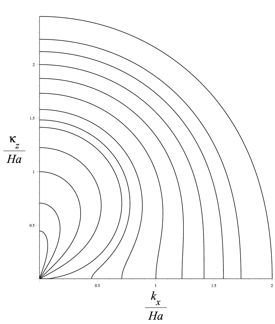
Cross-sections of the iso-$\lambda$ manifolds in the $k_{y}=0$ plane tell a different story (see Fig. 2). The geometry of this graph is formally identical to geometries of channel flow with transverse magnetic field [12], but with the roles of $\kappa_{z}$ and $k_{x}$ reversed. Both phenomenologies thus bear strong similarities, but for the orientation of the magnetic field. For small Ha, the flow is essentially isotropic, $k_{x}$ and $k_{y}$ have similar behaviours, and the manifolds are spheres. As Ha increases, the increasing suppression of the $k_{x}$ modes distorts the contours in the $k_{y}=0$ plane. This effect becomes more pronounced as Ha increases, until we obtain situations where the $k_{x}$ modes are almost entirely suppressed.
Conversely, for a fixed value of Ha, as the value of the largest eigenvalue (and so the number of modes under consideration) increases, we have the following sequence. Initially, the modes have $k_{x}$ strongly suppressed, and the flow is essentially 2D. Next, we enter a regime where the curves of constant $\lambda$ pass through the origin; this is the 3D, anisotropic regime. In this regime, all modes are contained outside a cone of axis $\mathbf{e}_{x}$, tangent to the manifold at the origin, whose half-angle is easily derived from (15) as $\theta_{J}=\pi/2-\cos^{-1}(\sqrt{-\lambda}/Ha)$. This phenomenology reflects that in MHD turbulence at high interaction parameter $S=\sigma B^{2}L/(\rho U)$, all energy-containing modes are expelled from the Joule cone [20, 8]. Finally, the contours split away from the origin and we reach the regime of weakly anisotropic 3D flow, which becomes more closely isotropic as the contours approach a semi-circular shape. We also see this from a different perspective in the following subsection.

Now consider the plot of attractor dimension vs Hartmann number for fixed Reynolds number. Figure 3 plots the dimension of the attractor for Reynolds numbers starting at $10$ and increasing in steps of $20$, for Hartmann number starting at $1$ and increasing in multiplicative steps of 1.2 up to a maximum value of approximately 4400.

We note that as in [11] this plot divides the plane up into three regions: a 3D quasi-isotropic region (I), a 3D anisotropic region (II), and a 2D region (III), corresponding to the classification given above.
For a fixed Reynolds number, and increasing Ha, the dimension initially depends only weakly on Hartmann number in the quasi-isotropic 3D region. When a critical value is reached, all iso-$\lambda$ manifolds cut through the origin: at this point, the attractor dimension undergoes a transition to the 3D anisotropic region where where it scales approximately as $\text{Ha}^{-1}$. From the data, we find that for low Reynolds numbers, the exponent is $-1\pm 0.1$, but as the Reynolds number increases the uncertainty reduced to about $-1\pm 0.003$, which strongly suggests that the slope tends to $-1$ at large Reynolds number.
For higher values of Ha, another phase transition occurs to the 2D state, where all modes become $x-$independent. Since their associated eigenvalue becomes independent of Ha (from (14)), so does the upper bound for the attractor dimension.
The transition from quasi-isotropic 3D to anisotropic 3D sets occurs for $d_{\rm att}\sim Ha^{3}$ in this diagram: this transition is quite gradual, and we can find the transition curve and its slope either by examining the data for the first mode with non-zero $k_{x}$, zero $k_{y}$ and $\kappa_{z}$ approximately 1.57, or by finding the number of modes for which $|\lambda|<\text{Ha}^{2}/2$. The two approaches give the results $d_{\rm att}\simeq(0.25\pm 0.01)\text{Ha}^{3\pm 0.003}$ and $d_{\rm att}\simeq(2.35\pm 0.01)\text{Ha}^{3.05\pm 0.05}$ respectively. The 2D region is that of all least dissipative modes for which $k_{x}=0$; this time, examining the data gives a scaling of the form $d_{\rm att}\simeq(2.2\pm 0.1)\text{Ha}^{1.03\pm 0.03}$ for this transition.

A similar approach is followed, holding Ha constant and varying Re, to determine how $d_{att}$ varies with Re in each of these three regions. Some sample curves are plotted on Fig. 3. Combining both graphs, we obtain that the upper bound for the attractor dimension follows one of three scalings:
In the 2D regime,

In the 3D anisotropic regime,

and in the 3D quasi-isotropic regime:

The scalings for $d_{\rm att}$ in 3D regimes are consistent with the upper bound obtained in periodic domains and with heuristic estimates for the number of degree of freedoms in the system as both $d_{\rm att}\sim\text{Re}^{4}/\text{Ha}$ in the limit as Re and Ha tend to infinity while remaining within the 3D regime, i.e. $Ha<<d_{\rm att}<<Ha^{3}$ [11]. This result is not a priori obvious from the mathematical point of view, since walls parallel to the magnetic fields make the spectral distribution of the modes strongly inhomogeneous, in contrast with flows in periodic domains and with channels perpendicular to the field. From the physical point of view, however, the fact that the attractor dimension is not significantly affected by the nature of the boundaries when Re is large enough, reflects that the number of degrees of freedom in the flow is mainly determined by turbulence far from the walls. In the 2D regime, $d_{\rm att}$ understandably behaves in the same way as in the fully periodic case, since in both cases, strictly 2D modes incur no Joule dissipation. In channels with walls perpendicular to the magnetic field, on the other hand, the Hartmann boundary layer that develops against the wall precludes strict two-dimensionality and significant Joule dissipation occurs there so that $d_{\rm att}$ continues to decrease with Ha in the quasi-2D regime.
A remark should be made on the value of the exponent of Re in the estimates for the $d_{\rm att}$. In the strongly anisotropic regime, for example, heuristic estimate for the number of degrees of freedom of turbulence in a periodic box yields $d_{M}\sim Re^{2}/Ha$ [11], and not $d_{M}\sim Re^{4}/Ha$. It was previously noted that this overestimate for the exponent of Re takes its roots in the loose upper bound for the inertial terms in (7). This issue is not specific to MHD flows but betrays a core difficulty in the derivation of tight upper bounds for attractor dimensions in 3D turbulence. Nevertheless, the exponent of Ha in the estimate for $d_{\rm att}$ coincides with the heuristic estimates in the geometries with periodic boundary conditions and channels perpendicular to the magnetic field in both 3D regimes. Since our numerical estimate shows that this exponent also remains valid in the case of a channel parallel to the magnetic field, it is likely to be a tight estimate in this case too.

References

- [1] N. Vetcha, S. Smolentsev, M. Abdou, and R. Moreau, Phys. Fluids 25, 024102 (2013).
- [2] P. H. Roberts, Introduction to Magnetohydrodynamics (Longmans, 1967).
- [3] H. K. Moffatt, J. Fluid Mech. 28, 571 (1967).
- [4] P. A. Davidson, J. Fluid Mech. 336, 123 (1997).
- [5] O. Zikanov and A. Thess, J. Fluid Mech. 358, 299 (1998).
- [6] A. Thess and O. Zikanov, J. Fluid Mech. 579, 383 (2007).
- [7] R. Klein and A. Pothérat, Phys. Rev. Lett. 104, 034502 (2010).
- [8] A. Pothérat, Magnetohydrodynamics 48, 13 (2012).
- [9] A. Pothérat and R. Klein, J. Fluid Mech. 761, 168 (2014).
- [10] A. Alemany, R. Moreau, P. Sulem, and U. Frish, Journal de Mécanique 18, 277 (1979).
- [11] A. Pothérat and T. Alboussière, Phys. Fluids 15, 3170 (2003).
- [12] A. Pothérat and T. Alboussière, Phys. Fluids 18, 125102 (2006).
- [13] V. Dymkou and A. Pothérat, J. Theor. Comp. Fluid Mech. 23, 535 (2009).
- [14] K. Kornet and A. Pothérat, accepted for publication in J. Comp. Phys. , arXiv:1403.4129 (2015).
- [15] C. R. Doering and J. D. Gibbons, Applied Analysis of the Navier-Stokes Equation (Cambridge University Press, 1995).
- [16] A. Pothérat and V. Dymkou, J. Fluid Mech. 655, 174 (2010).
- [17] D. Krasnov, M. Rossi, O. Zikanov, and T. Boeck, J. Fluid Mech. , 73 (2008a).
- [18] D. Krasnov, O. Zikanov, J. Schumacher, and T. Boeck, Phys. Fluids 20, 095105 (2008b).
- [19] P. Constantin, C. Foias, O. P. Mannley, and R. Temam, Memoirs of the Am. Math. Soc. 53 (1985).
- [20] B. Knaepen and R. Moreau, Ann. Rev. Fluid. Mech. 40, 25 (2008).
- [21] S. Eckert, G. Gerbeth, W. Witke, and H. Langenbrunner, Int. J. Heat Fluid Flow , 358 (2001).