Form factors and decay rate of decays in the QCD sum rules
Rare exclusive decays are analyzed in the framework of the three–point QCD sum rules approach. The two gluon condensate corrections to the correlation function are included and the form factors of this transition are evaluated. Using the form factors, the decay width and integrated decay rate for these decays are also calculated.
I Introduction
The rare flavor-changing neutral-current (FCNC) processes {} are widely studied to test the predictions of Standard Model (SM) at loop level and to search for new-physics (NP). The recent theoretical studies can be found in the Refs.[1]-[6].
Various physical observables of leptonic, semileptonic and radiative decays have been measured by LHCb. For instance, the form factor, independent observables in the decay [7] and the the asymmetry in decays [8] have been measured. More recent measurements in the LHCb for FCNC transitions can be seen in Refs.[9]-[11]. Measurements of various observables at LHCb indicate that SM predictions are in good agreement with the experimental results. Therefore, most of the new physics scenarios are excluded.
Rare proceeds FCNC transitions. This decay has not yet been measured by LHCb. There is not theoretical studies relevant to the form factors and decay rate of this decay. We try to calculate the form factors and the decay rate of decay as well. We use the three–point QCD sum rules approach in the calculation of these form factors. The QCD sum rules have widely been used to calculate form factors (some similar studies can be found in Refs.[12]-[19]).
The paper includes 3 sections: In section 2, we recall the effective Hamiltonian and use the three–point QCD sum rules approach to calculate these form factors. In section 3, we will use the numerical values of form factors in order to determine the sensitivity of the decay rate to the invariant dileptonic mass and then present our conclusion.
II Sum rules for the transition form factors
The matrix element of the transition can be written as:
| (1) |
where
and and are Wilson coefficients evaluated in the naive dimensional regularization (NDR) scheme at the leading order (LO), next to leading order (NLO) and next-to-next leading order (NNLO) in the SM[20]–[27]. , where contains both the perturbative part and long-distance part . in [20] is as follows:
| (2) | |||||
| (3) |
and the function is defined in [20]. Here, – are the Wilson Coefficients in the leading logarithmic approximation. The relevant Wilson Coefficients are given in [29]. involves resonances [21, 30, 31], where are the vector charmonium states. Following refs. [21, 30], is as follows:
| (4) |
where and takes different value for different exclusive semileptonic decays. This phenomenological parameters can be fixed for decay by equating the naive factorization estimate of the rate and the results of the experimental measurements [29]. For the time being, there is no experimental result on . Thus, we use the results of to estimate the values of in our numerical calculations i.e, for and for , respectively.
Relevant properties of vector charmonium states are summarized in Table 1.
| Mass[ GeV] | [ MeV] | |||
|---|---|---|---|---|
| for | ||||
| for | ||||
| for | ||||
| for | ||||
| for | ||||
| for | ||||
| for | ||||
The transition amplitude of the exclusive decays is obtained by sandwiching Eq.(1) between the initial meson state and the final meson state in terms of form factors as follows:
| (5) | |||||
where is the polarization vector of meson, and are momentums of the and mesons, respectively. Taking the Lorentz invariance and parity conservation into account, the matrix elements of the Eq.(5) are parameterized in terms of the form factors as follows:
| (6) |
| (7) | |||||
| , |
where , , , , , and are the transition form factors. and , here, is transfer momentum or the momentum of the boson (photon).
The transition amplitude in terms of the form factors is as follows:
| (8) | |||||
where
| (9) |
The decay rate for the decay is obtained as follows:
| (10) |
where
| (11) |
| (12) | |||||
We follow the QCD sum rules approach to calculate the aforementioned form factors. The QCD sum rules start with the following correlation functions:
| (13) |
where and are interpolating currents of the and meson states, respectively. and consist of the vector (), axial vector (), tensor () and pseudo tensor () transition currents. The above correlation functions can be re-written by inserting the two complete sets of the and meson currents with the same quantum numbers into the Eq. (13) as follows:
| (14) |
where ”” indicates higher states and continuum contributions. The and matrix elements are as follows:
| (15) |
where and are the leptonic decay constants of the and mesons, respectively. Using Eq.(6), Eq.(7) and Eq.(15) together with the summation over the polarization of the meson, the Eq.(14) can be re-written as follows:
| (16) | |||||
Then, on the QCD or theoretical side, the correlation functions are evaluated in terms of the quarks and gluons parameters by means of the the operator product expansion (OPE). The correlation functions are written as:
| (17) |
where each with and contains the perturbative and nonpertubative parts as:
| (18) |
The perturbative part of the Eq.(18) is the bare-loop diagram given in Fig.1(a). The nonperturbative part consists of the light quark condensates and the two gluon condensates diagrams {see Fig.2(a-f)}. Contributions of the light quark condensates {diagrams shown in Fig.1(b, c, d)} are removed by the application of the double Borel transformations [18]. Therefore, the two gluon condensates diagrams shown in Fig.2(a-f) are described as the first correction.

The bare-loop contributions for each structure in the correlation function are the double dispersion integrals given in the following formula:
| (19) |
In the foregoing calculations of the spectral density , Cutkosky Rules are applied to the Feynman Integrals. According to these rules the quark propagators are replaced by Dirac Delta Functions: which means that all quarks are real.
The integration region in Eq.(19) is restricted by the arguments of the three functions in and space coordinates, where these functions must be zero at the same time. As a result, the following inequality in and space coordinates is obtained:
| (20) |
where .
Following the required calculations, the spectral densities are obtained as:
| (21) | |||||
where
| (22) |
Now, the aim here is to evaluate the nonperturbative part of the Eq.(18). As has already been mentioned, the contributions of the the light quark condensate diagrams (Fig. 1b,1c and 1d) to the nonperturbative part of the correlation function vanish[18]. Thus, the gluon condensates diagrams shown in Fig.2 are evaluated. The Fock–Schwinger fixed–point gauge [32, 33, 34] is used, where is the gluon field.
The following integrals must be solved while evaluating the gluon condensate diagrams: [17, 35]:
| (23) |
where is the momentum of the spectator quark .
The integrals are transferred from Minkowski space–time to Euclidean space–time. Then, the Schwinger representation for the Euclidean propagator is used as in the following:
| (24) |
The Eq.(24) is convenient to perform the Borel transformation, that is:
| (25) |
Performing integration over loop momentum and auxiliary parameters used in the exponential representation of propagators [33], and applying double Borel transformations over and , the transformed form of the integrals (see also [33]) in Eq.(23) can be written as:

| (26) | |||||
where
| (27) |
where and are the Borel parameters.
The function is:
where
| (28) |
The Borel transformed form of the phenomenological side {Eq. (16)} and QCD side {Eq. (17)} is calculated. The QCD sum rules for the form factors ( , , , , , and ) can be achieved by equating the expressions of the phenomenological side {Eq. (16)} and QCD side {Eq. (17)} just after the following Borel transformation:
| (29) | |||||
| (30) | |||||
Note that, the Borel transformation suppresses the contributions of higher states and continuum. In addition, the two gluon condensates contributions are and . The contributions of the aforementioned expressions ( and ) are considered in the numerical analysis. However, since each of these explicit expressions is extremely long, it is found unnecessary to show them all in this study. Therefore, one of these expressions () is shown as a sample in Appendix. The and are the continuum thresholds in and channels, respectively. Also and .
III Numerical analysis
From the explicit expressions for the decay rate, it is clear that the main input parameters entering into the expressions are Wilson coefficients , and , the CKM matrix elements , [28] and the form factors , , , , , , . Moreover, the value of the gluon condensate [36], the masses and leptonic decay constants, GeV[28], Mev[28], and MeV[28], the masses of the quarks , [28] , and [28] are necessary for evaluation of the form factors.
In order to reduce the theoretical uncertainties as well as the dependence on the input parameters used in the calculation of the form factors the same set of the input parameters is utilized for calculation of the form factors and the decay constant at the same time. We obtain MeV by using generic formula given in Ref. [37]. This result is in good agreement with the results of the Ref.[38], which is MeV. Furthermore, the form factors contain four auxiliary parameters: the Borel mass squares and and the continuum threshold and . The physical quantities such as form factors are supposed to be independent or weakly dependent on these auxiliary parameters in the so called ”working regions”.
The upper bound of the ”working region” of and is chosen in a way that the contribution of continuum is less than that of the first resonance. The lower bound of is fixed so that the contributions proportional to the highest power of are less than about of the contributions proportional to the highest power of . With the aforementioned conditions, we find the stable region for the form factor in the following intervals; and . The continuum thresholds, and are determined by the mass of the corresponding ground-state hadron. The value of the and must be less than the energy of the first excited states with the same quantum numbers. Hence, the following regions for the and are used: and .
In order to estimate the decay width of decays, the dependency of the form factors , , , , , and in the whole physical region, , is required.
The detailed numerical analysis of the form factor depicts that the dependence of the form factors fits into the following function:
| (31) |
The parameters of the fit function are given in Table 2:
The errors in the numerical calculation shown in Table II stem from the variation of the continuum thresholds, the Borel mass parameter in the given intervals and the uncertainties of the input parameters.
Taking account of the dileptonic invariant mass( ) dependence of the form factors in the kinematical allowed region in the range of , we study the the differential decay rate for the decays. Our results for three different values of the are presented in Table 3. In addition, Fig. (3) depicts the dependence of the differential decay rate on for full kinematical allowed region.
The branching ratio can be calculated if we know the mean life time of the . There is no experimental data on the mean life time of the . Thus, we ignore about the calculation of the banting ratio. It is worth mentioning that using the theoretical methods like Bethe-Salpeter model [39] and potential model [40], it is possible to calculate the mean life time of the meson and estimate the branching ratio as well.
| GeV | ) |
|---|---|
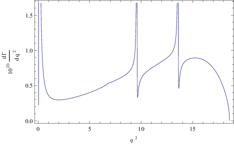
Finally, we calculate the integrated decay rate for the decays as follows:
| (32) |
To sum up, we investigated the decays in the framework of the QCD sum rules approach. The form factors of these decays were obtained in terms of the . The contributions of the quark condensates in the correlations function found to be zero, so the contributions of the two gluon condensates to the correlations function were evaluated. Finally, we calculated the differential decay width and the integrated decay rate of these decays for the muon channel.
References
- [1] D. Cogollo, F. S. Queiroz and P. Vasconcelos, arXiv:1312.0304 [hep-ph].
- [2] X. -Q. Li, Y. -D. Yang and X. -B. Yuan, arXiv:1311.2786 [hep-ph].
- [3] A. J. Buras and J. Girrbach, FLAVOUR(267104)-ERC-50 [arXiv:1309.2466 [hep-ph]].
- [4] A. Ali, A. Y. .Parkhomenko and A. V. Rusov, arXiv:1312.2523 [hep-ph].
- [5] F. ço. Richard, arXiv:1312.2467 [hep-ph].
- [6] G. C. Branco and M. N. Rebelo, PoS Corfu 2012, 024 (2013) [arXiv:1308.4639 [hep-ph]].
- [7] RAaij et al. [LHCb Collaboration], Phys. Rev. Lett. 111, 191801 (2013) [arXiv:1308.1707 [hep-ex]].
- [8] R. Aaij et al. [LHCb Collaboration], Phys. Rev. Lett. 111, 151801 (2013) [arXiv:1308.1340 [hep-ex]].
- [9] RAaij et al. [LHCb Collaboration], Phys. Rev. Lett. 111, 101805 (2013) [arXiv:1307.5024 [hep-ex]].
- [10] M. Vesterinen [LHCb Collaboration], PoS Beauty 2013, 005 (2013) [arXiv:1306.0092 [hep-ex]].
- [11] R. Aaij et al. [LHCb Collaboration], JHEP 1308, 131 (2013) [arXiv:1304.6325 [hep-ex]].
- [12] V. Bashiry, arXiv:1305.6535 [hep-ph].
- [13] N. Ghahramany and A. R. Houshyar, Acta Phys. Polon. B 44, no. 9, 1857 (2013).
- [14] L. -F. Gan, Y. -L. Liu, W. -B. Chen and M. -Q. Huang, Commun. Theor. Phys. 58, 872 (2012) [arXiv:1212.4671 [hep-ph]].
- [15] Y. Sarac, K. Azizi and H. Sundu, Nucl. Phys. Proc. Suppl. 245, 164 (2013).
- [16] A. Khodjamirian, C. .Klein, T. .Mannel and N. Offen, Phys. Rev. D 80, 114005 (2009) [arXiv:0907.2842 [hep-ph]].
- [17] T. M. Aliev and M. Savci, Eur. Phys. J. C 47, 413 (2006) [hep-ph/0601267].
- [18] K. Azizi, F. Falahati, V. Bashiry and S. M. Zebarjad, Phys. Rev. D 77, 114024 (2008) [arXiv:0806.0583 [hep-ph]].
- [19] R. S. Marques de Carvalho, F. S. Navarra, M. Nielsen, E. Ferreira and H. G. Dosch, Phys. Rev. D 60, 034009 (1999) [hep-ph/9903326].
- [20] A. J. Buras and M. Munz, Phys. Rev. D 52, 186 (1995) [arXiv:hep-ph/9501281].
- [21] C. S. Lim, T. Morozumi and A. I. Sanda, Phys. Lett. B 218, 343 (1989).
- [22] W. S. Hou, R. S. Willey and A. Soni, Phys. Rev. Lett 58 (1987) 1608; ibid 60 (1988) 2337 Erratum.
- [23] N. G. Deshpande and J. Trampetic, Phys. Rev. Lett 60 (1988) 2583.
- [24] M. Jezabek and J. H. Kühn, Nucl. Phys. B320 (1989) 20.
- [25] M. Misiak, Nucl. Phys. B393 1993 23.
- [26] M. Misiak, Nucl. Phys. B439 461(E) 1995.
- [27] T. Huber, E. Lunghi, M. Misiak and D. Wyler, Nucl. Phys. B740 (2006) 105.
- [28] J. Beringer et al. (Particle Data Group), Phys. Rev. D86, 010001 (2012)
- [29] A. Ali, P. Ball, L. T. Handoko and G. Hiller, Phys. Rev. D 61, 074024 (2000) [arXiv:hep-ph/9910221].
- [30] A. Ali, T. Mannel and T. Morozumi, Phys. Lett. B 273, 505 (1991).
- [31] F. Kruger and L. M. Sehgal, Phys. Lett. B 380, 199 (1996) [arXiv:hep-ph/9603237].
- [32] V. A. Fock, Sov. Phys. 12, 404 (1937).
- [33] J. Schwinger, Phys. Rev. 82, 664 (1951).
- [34] V. Smilga, Sov. J. Nucl. Phys. 35, 215 (1982).
- [35] V. V. Kiselev, A. K. Likhoded, A. I. Onishchenko, Nucl. Phys. B 569 (2000) 473.
- [36] M. A. Shifman, A. I. Vainshtein, V. I. Zakharov, Nucl. Phys. B147 (1979) 385.
- [37] V. Bashiry, K. Azizi and S. Sultansoy, Phys. Rev. D 84, 036006 (2011) [arXiv:1104.2879 [hep-ph]].
- [38] Z. -G. Wang, Eur. Phys. J. A 49 (2013) 131 [arXiv:1203.6252 [hep-ph]].
- [39] A. Abd El-Hady, M. A. K. Lodhi and J. P. Vary, Phys. Rev. D 59, 094001 (1999) [hep-ph/9807225].
- [40] V. V. Kiselev, A. E. Kovalsky and A. I. Onishchenko, Phys. Rev. D 64, 054009 (2001) [hep-ph/0005020].
Appendix
In this section, we present the explicit expressions for the coefficients corresponding to the gluon condensates contributions of structure entering to the expressions for the form factors in Eq.(29).
| (33) | |||||
| (34) |
where