The Fourier estimation method with positive semi-definite estimators

Jirô Akahori , Nien-Lin Liu , Maria Elvira Mancino and Yukie Yasuda Jirô Akahori, Nien-Lin Liu and Yukie Yasuda Department of Mathematical Sciences, Ritsumeikan University 1-1-1 Nojihigashi, Kusatsu, Shiga, 525-8577, Japan Maria Elvira MancinoDepartment of Economics and Management, University of Firenze, Via delle Pandette, 9, Firenze, Italy

Date: October, 2014

Abstract.

In this paper we present a slight modification of the Fourier estimation method of the spot volatility (matrix) process of a continuous Itô semimartingale where the estimators are always non-negative definite. Since the estimators are factorized, computational cost will be saved a lot.

1. Introduction

In this paper we present a slight modification of the Fourier estimation method of the spot volatility (matrix) process of an Itô semimartingale. The method is originally introduced by Paul Malliavin and the third author in [3, 4]. The main aim of the modification is to construct an estimator of the matrix which always stays non-negative definite.

A motivation of the present study is to make an implementation of the Fourier method easier when it is applied to “dynamic principal component analysis”, an important application of the spot volatility estimation (see [1, 2]). Due to the lack of symmetry of the matrices, its estimated eigenvalues are sometimes non-positive, or even worse, non-real. This is not the case with those based on finite differences (FD) of the integrated volatility such as Ngo-Ogawa’s method [6]. However, as the Fourier method has many advantages over the FD ones, among which robustness against non-synchronous observations counts most, the modification to be presented in this paper would be important.

There is a by-product of the modification; thanks to a symmetry imposed to have the non-negativity our estimator is factorized, which may save computational cost a lot.

The present paper is organized as follows. We will firstly introduce a generic form of Fourier type estimators (Definition 1), and discuss how it works as a recall (section 2.2). After remarking that the classical one is obtained by a choice of the “fiber” (Remark 2), we will introduce a class of such estimators (section 3), each of which is labeled by a positive definite function. As a main result, we will prove its positive semi-definiteness (Theorem 4). In addition, we give a remark (Remark 5) that with an action of finite group, some of the newly introduced positive semi-definite estimators reduce to the classical one.

In section 3.2, we will give a factorized representation of the estimator (Definition 6) which is parameterized by a measure by way of Bochner’s correspondence. The use of the expression may reduce the computation cost, as will be exemplified by simple experiments presented in section 4. Section 3.3 gives an important remark that as a sequence of estimators, the parameterization measures should be a delta-approximating kernel. Three examples of the kernels are given (Examples 1–3), two of which are used in the simple experiments presented in section 4.

In the present paper, we will not study limit theorems; consistency nor central limit theorem in detail. More detailed studies in these respects will appear in another paper.

Acknowledgment

This work was partially supported by JSPS KAKENHI Grant Numbers 25780213, 23330109, 24340022, 23654056 and 25285102.

2. The Fourier Method Revisited

2.1. Generic Fourier Estimator

Let $X=(X^{1},\cdots,X^{d})$ be a $d$ -dimensional continuous semimartingale. Suppose that its quadratic variation (matrix) process is absolutely continuous in $t$ almost surely. In this paper, we are interested in a statistical estimation of the so-called spot volatility process;

\frac{d[X^{j},X^{j^{\prime}}]_{t}}{dt}(\omega)=:V^{jj^{\prime}}_{t}(\omega),\quad 0\leq t\leq 1,\ 1\leq j,j^{\prime}\leq d,

as a function in $t$ , especially when $d\geq 2$ , for a given observations of $X^{j}$ on a partition $\Delta^{j}:0=t^{j}_{0}<\cdots<t^{j}_{N_{j}}=1$ , $j=1,\cdots,d$ .

Here and hereafter we normalize the time interval to $[0,1]$ for notational simplicity.

We start with a generic form of a Fourier estimator with respect to this observation set, to have a unified view.

Definition 1.

Let $\mathcal{K}$ be a finite subset of $\mathbf{Z}$ , $\mathcal{S}=\{\mathcal{S}(k)\subset_{\mathrm{finite}}\mathbf{Z}^{2}:k\in{\mathcal{K}},(s,s^{\prime})\in\mathcal{S}(k)\Rightarrow s+s^{\prime}=k\}$ be a “fiber” on $\mathcal{K}$ , and $c$ be a complex function on $\mathcal{K}$ . A Fourier estimator associated with $(\mathcal{K},\mathcal{S},c)$ is a $d\times d$ matrix defined entry-wisely by

(2.1)

\begin{split}&(V_{(\mathcal{K},\mathcal{S},c)})_{j,j^{\prime}}(t)\\ &=\sum_{l=1}^{N_{j}}\sum_{l^{\prime}=1}^{N_{j^{\prime}}}\sum_{k\in\mathcal{K}}c(k)e^{2\pi ikt}\sum_{(s,s^{\prime})\in\mathcal{S}(k)}e^{-2\pi ist_{l}^{j}}e^{-2\pi is^{\prime}t_{l^{\prime}}^{j^{\prime}}}\Delta X^{j}_{l}\Delta X^{j^{\prime}}_{l^{\prime}},\\ &\hskip 113.81102pt(1\leq j,j^{\prime}\leq d),\end{split}

where

\Delta X^{j}_{l}:=X^{j}_{t^{j}_{l}}-X^{j}_{t^{j}_{l-1}}.

Remark 2.

If we take $\mathcal{K}=\{0,\pm 1,\cdots,\pm L\}$ for some positive integer $L$ , $\mathcal{S}(k)=\{(s,s^{\prime})|s+s^{\prime}=k,s=0,\pm 1,\cdots,\pm M\}$ for some positive integer $M$ , and $c(k)=(1-\frac{|k|}{L+1})/(2M+1)$ , then the estimator $V_{(\mathcal{K},\mathcal{S},c)}$ coincides with the one introduced in [4]. In fact, with these parameters, we have

(2.2)

\begin{split}&(V)_{j,j^{\prime}}(t)=\sum_{k=-L}^{L}\left(1-\frac{|k|}{L+1}\right)e^{2\pi ikt}\\ &\cdot\frac{1}{2M+1}\sum_{s=-M}^{M}\sum_{l=1}^{N_{j}}\sum_{l^{\prime}=1}^{N_{j^{\prime}}}e^{-2\pi ist^{j}_{l}}e^{-2\pi i(k-s)t^{j^{\prime}}_{l^{\prime}}}\Delta X^{j}_{l}\Delta X^{j^{\prime}}_{l^{\prime}}.\end{split}

With the Dirichlet and the Fejér kernels;

D_{M}(x)=\sum_{|s|\leq M}e^{2\pi isx}=\frac{\sin(2M+1)\pi x}{\sin\pi x},

and

\begin{split}K_{L}(x)&:=\frac{1}{L}\sum_{M=0}^{L-1}D_{M}(x)=\sum_{|k|\leq L-1}\left(1-\frac{|k|}{L}\right)e^{2\pi ikx}\\ &=\frac{1}{L}\left(\frac{\sin(L\pi x)}{\sin(\pi x)}\right)^{2},\end{split}

we can rewrite (2.2) as

(2.3)

\begin{split}&(V)_{j,j^{\prime}}(t)\\ &=\frac{1}{(2M+1)}\sum_{l,l^{\prime}}K_{L+1}(t-t^{j}_{l})D_{M}(t^{j}_{l}-t^{j^{\prime}}_{l^{\prime}})\Delta X^{j}_{l}\Delta X^{j^{\prime}}_{l^{\prime}}\\ &=\frac{1}{(2M+1)}\sum_{l,l^{\prime}}\left(\frac{\sin\{(L+1)\pi(t-t^{j}_{l})\})}{\sin(\pi(t-t^{j}_{l}))}\right)^{2}\frac{\sin\{(2M+1)\pi(t^{j}_{l}-t^{j^{\prime}}_{l^{\prime}})\}}{\sin\pi(t^{j}_{l}-t^{j^{\prime}}_{l^{\prime}})}\\ &\hskip 113.81102pt\cdot\Delta X^{j}_{l}\Delta X^{j^{\prime}}_{l^{\prime}}.\end{split}

2.2. A Heuristic Derivation

Here we give a heuristic explanation of the idea behind the Fourier method, which was originally proposed in [3, 4], and now is extended to (2.1) to include a class of positive semi-definite estimators that will be introduced in the next section.

Looking at (2.1) or (2.2) carefully, we notice that though naively, we may suppose

(2.4)

\begin{split}&(V_{(\mathcal{K},\mathcal{S},c)})_{j,j^{\prime}}(t)\\ &\sim\sum_{k\in\mathcal{K}}c(k)e^{2\pi ikt}\sum_{(s,s^{\prime})\in S(k)}\left(\int_{0}^{1}e^{-2\pi isu}dX^{j}_{u}\right)\left(\int_{0}^{1}e^{-2\pi is^{\prime}u}dX^{j^{\prime}}_{u}\right)\\ &=\sum_{k\in K}c(k)|\mathcal{S}(k)|e^{2\pi ikt}\int_{0}^{1}e^{-2\pi iku}d[X^{j},X^{j^{\prime}}]_{u}\\ &+\sum_{k\in K}c(k)e^{2\pi ikt}\int_{0}^{1}\int_{0}^{u}\sum_{(s,s^{\prime})\in\mathcal{S}(k)}(e^{-2\pi isu}e^{-2\pi is^{\prime}v}dX^{j}_{u}dX^{j^{\prime}}_{v}\\ &\hskip 170.71652pt+e^{-2\pi is^{\prime}u}e^{-2\pi isv}dX^{j^{\prime}}_{u}dX^{j}_{v})\\ &=:I+II.\end{split}

The term $I$ can be understood to be a weighted partial sum of Fourier series of $V^{jj^{\prime}}$ , which may converge uniformly if the weight $c(k)|\mathcal{S}(k)|$ is properly chosen (in the case of (2.2), it is Fejér kernel). The term $II$ vanishes, roughly because, $\sum_{(s,s^{\prime})\in S(k)}(e^{-2\pi isu}e^{-2\pi is^{\prime}v}$ behaves like a Dirichlet kernel $D(u-v)$ , which converges weakly to the delta measure.

3. Positive Semi-Definite Fourier Estimators

In financial applications, we are often interested in computing the rank of the (spot) volatility matrix. Since it is positive semi-definite the rank is estimated by a hypothesis testing on the number of positive eigenvalues. The estimator (2.2), or equivalently given as (2.3), however, sometimes fails to be symmetric¹¹ 1 This is seen from the following simple observation: $\sum_{l=1}^{2}\sum_{l^{\prime}=1}^{2}a_{l,l^{\prime}}(x^{1}_{l}x^{2}_{l^{\prime}}-x^{2}_{l}x^{1}_{l^{\prime}})=(a_{1,2}-a_{2,1})(x_{1}^{1}x_{2}^{2}-x_{1}^{2}x_{2}^{1})$ . since $K_{M}(t-t_{l})D_{L}(t_{l}-t_{l^{\prime}})$ is not symmetric in $l,l^{\prime}$ , and thus its eigenvalues are not always real numbers. This causes some trouble in estimating the rank of the volatility matrix. Here we propose a class of Fourier estimators that will be proven to be symmetric and positive semi-definite.

Remark 3.

We just note that the positive semi-definiteness of the Fourier estimator defined in [4] of the integrated volatility matrix (the $0$ -th coefficient) is proved in [5].

3.1. Positive Fourier Estimators

The main result of the present paper is the following

Theorem 4.

Suppose that $\mathcal{K}=\{0,\pm 1,\cdots,\pm 2M\}$ for some positive integer $M$ , $c$ is a positive semi-definite function on $\mathcal{K}$ , and

\begin{split}&\mathcal{S}(k)=\\ &\begin{cases}\{(-M+k+v,M-v):v=0,\cdots,2M-k\}&0\leq k\leq 2M\\ \{(M+k-v,-M+v:v=0,\cdots,2M+k\}&-2M\leq k<0.\end{cases}\end{split}

Then, $V_{(\mathcal{K},\mathcal{S},c)}$ defined in (2.1) is positive semi-definite.

Proof.

Let $a_{j}$ , $j=1,2,3$ be arbitrary functions on $\mathbf{Z}$ . From the definitions of $(\mathcal{K},\mathcal{S})$ , we notice that

\begin{split}&\sum_{k\in\mathcal{K}}\sum_{(s,s^{\prime})\in\mathcal{S}(k)}a_{1}(k)a_{2}(s)a_{3}(s^{\prime})\\ &=\sum_{k=0}^{2M}\sum_{v=0}^{2M-k}a_{1}(k)a_{2}(-M+k+v)a_{3}(M-v)\\ &+\sum_{k=-2M}^{-1}\sum_{v=0}^{2M+k}a_{1}(k)a_{2}(M+k-v)a_{3}(-M+v)=:A+B\end{split}

For the first term of the right-hand-side,

\begin{split}A&=\sum_{k=0}^{2M}\sum_{u=k-M}^{M}a_{1}(k)a_{2}(k-u)a_{3}(u)\\ &=\sum_{u=-M}^{M}\sum_{k=0}^{u+M}a_{1}(k)a_{2}(k-u)a_{3}(u)\\ &=\sum_{u=-M}^{M}\sum_{u^{\prime}=-u}^{M}a_{1}(u+u^{\prime})a_{2}(u^{\prime})a_{3}(u),\end{split}

where we set $u=M-v$ in the first line, changed the order of the summations in the second line, and put $u^{\prime}=k-u$ . Similarly, we have

\begin{split}B&=\sum_{k=-2M}^{-1}\sum_{u=-M}^{M+k}a_{1}(k)a_{2}(k-u)a_{3}(u)\\ &=\sum_{u=-M}^{M}\sum_{k=u-M}^{-1}a_{1}(k)a_{2}(k-u)a_{3}(u)\\ &=\sum_{u=-M}^{M}\sum_{u^{\prime}=-M}^{-u-1}a_{1}(u+u^{\prime})a_{2}(u^{\prime})a_{3}(u).\end{split}

Thus we see that

(3.1)

\sum_{k\in\mathcal{K}}\sum_{(s,s^{\prime})\in\mathcal{S}(k)}a_{1}(k)a_{2}(s)a_{3}(s^{\prime})=\sum_{u=-M}^{M}\sum_{u^{\prime}=-M}^{M}a_{1}(u+u^{\prime})a_{2}(u^{\prime})a_{3}(u).

Applying (3.1) when $a_{1}(k)=c(k)e^{2\pi ikt}$ , $a_{2}(s)=e^{-2\pi ist^{j^{\prime}}_{l^{\prime}}}$ and $a_{3}(s^{\prime})=e^{-2\pi is^{\prime}t^{j}_{l}}$ , we obtain

(3.2)

\begin{split}&(V_{(\mathcal{K},\mathcal{S},c)})_{j,j^{\prime}}(t)\\ &=\sum_{l=1}^{N_{j}}\sum_{l^{\prime}=1}^{N_{j^{\prime}}}\sum_{u=-M}^{M}\sum_{u^{\prime}=-M}^{M}c(u-u^{\prime})e^{2\pi iu(t-t_{l}^{j})}e^{-2\pi iu^{\prime}(t-t_{l^{\prime}}^{j^{\prime}})}\Delta X^{j}_{l}\Delta X^{j^{\prime}}_{l^{\prime}}\\ &\hskip 113.81102pt(1\leq i,j\leq d).\end{split}

Here we used an obvious change of variables $u^{\prime}\mapsto-u^{\prime}$ .

Now the positive definiteness follows easily. In fact, for $x\in\mathbb{C}^{d}$ , we have

\begin{split}&\sum_{j,j^{\prime}}(V_{(\mathcal{K},\mathcal{S},c)})_{j,j^{\prime}}(t)x_{j}\overline{x_{j^{\prime}}}\\ &=\sum_{u=-M}^{M}\sum_{u^{\prime}=-M}^{M}c(u-u^{\prime})\\ &\cdot\left(\sum_{j=1}^{d}x_{j}\sum_{l=1}^{N_{j}}e^{2\pi iu(t-t_{l}^{j})}\Delta X^{j}_{l}\right)\left(\sum_{j^{\prime}=1}^{d}\overline{x_{j^{\prime}}}\sum_{l=1}^{N_{j^{\prime}}}e^{-2\pi iu^{\prime}(t-t_{l^{\prime}}^{j^{\prime}})}\Delta X^{j^{\prime}}_{l^{\prime}}\right)\\ &=\sum_{u=-M}^{M}\sum_{u^{\prime}=-M}^{M}c(u-u^{\prime})f(u)\overline{f(u^{\prime})}\geq 0,\end{split}

where we have put

f(u):=\sum_{j=1}^{d}x_{j}\sum_{l=1}^{N_{j}}e^{2\pi iu(t-t_{l}^{j})}\Delta X^{j}_{l}.

∎

Remark 5.

If we set in (3.2) $N:=N_{j}=N_{j^{\prime}}=2M+1$ , $\Delta t^{j}_{l}\equiv 1/N$ , and $c(k)=1-\min(|k|,|N-k|)/M$ , the estimator (3.2) coincides with (2.2) with $L=M$ . In fact, writing $t_{l}=l/N$ for $l=1,\cdots,N$ , we notice that, for $t=l_{0}/N$ ,

\begin{split}&(V_{(\mathcal{K},\mathcal{S},c)})_{j,j^{\prime}}(t)\\ &=\frac{1}{N}\sum_{l,l^{\prime}}\Delta X^{j}_{l}\Delta X^{j^{\prime}}_{l^{\prime}}\sum_{k=-M}^{M}\sum_{s=-M}^{M}c(k-s)e^{\frac{2\pi ik(l_{0}-l)}{N}}e^{-\frac{2\pi is(l_{0}-l^{\prime})}{N}},\\ \end{split}

and by the change of variables $(k,s)\mapsto(k-s,-s)$ , which is an automorphism over $\mathbb{Z}/N\mathbb{Z}$ , we have

\begin{split}&=\frac{1}{N}\sum_{l,l^{\prime}}\Delta X^{j}_{l}\Delta X^{j^{\prime}}_{l^{\prime}}\sum_{k=-M}^{M}\sum_{s=-M}^{M}c(k)e^{\frac{2\pi ik(l_{0}-l)}{N}}e^{\frac{2\pi is(l-l^{\prime})}{N}}.\end{split}

3.2. Parameterization by measures

By Bochner’s theorem, we know that for each positive semi-definite function $c$ , there exists a bounded measure $\mu$ on $\mathbf{R}$ such that

(3.3)

c(x)=\int_{\mathbf{R}}e^{2\pi iyx}\,\mu(dy).

Therefore, we may rewrite the positive Fourier estimator (3.2) using the measure $\mu$ instead of the positive semi-definite function $c$ . The expression in terms of the measure $\mu$ will be useful when implementing the Fourier method in estimating a spot volatility matrix.

Definition 6.

Let $\mu$ be a bounded measure and $M$ be a positive integer. We associate with $(\mu,M)$ an estimator of the spot volatility matrix as:

(3.4)

\begin{split}&(V_{(\mu,M)})_{j,j^{\prime}}(t)=\int_{\mathbf{R}}\left(\sum_{l=1}^{N_{j}}D_{M}(t-t_{l}^{j}+y)\Delta X^{j}_{l}\right)\\ &\hskip 113.81102pt\cdot\left(\sum_{l^{\prime}=1}^{N_{j^{\prime}}}D_{M}(t-t_{l^{\prime}}^{j^{\prime}}+y)\Delta X^{j^{\prime}}_{l^{\prime}}\right)\mu(dy),\\ &\hskip 170.71652pt(1\leq j,j^{\prime}\leq d).\end{split}

Remark 7.

Under the assumptions in Theorem 4 with the relation (3.3), we have that $V_{(\mathcal{K},\mathcal{S},c)}(t)=V_{(\mu,M)}(t)$ for all $t\in[0,1]$ . In fact, we have

\begin{split}&(V_{(\mathcal{K},\mathcal{S},c)})_{j,j^{\prime}}(t)\\ &=\sum_{\begin{subarray}{c}1\leq l\leq N_{j}\\ 1\leq l^{\prime}\leq N_{j^{\prime}}\end{subarray}}\int_{\mathbf{R}}\sum_{|k|\leq M}\sum_{|s|\leq M}e^{2\pi i(t-t_{l}^{j}+y)k}e^{-2\pi i(t-t_{l^{\prime}}^{j^{\prime}}+y)s}\mu(dy)\Delta X^{j}_{l}\Delta X^{j^{\prime}}_{l^{\prime}}\\ &=\sum_{\begin{subarray}{c}1\leq l\leq N_{j}\\ 1\leq l^{\prime}\leq N_{j^{\prime}}\end{subarray}}\int_{\mathbf{R}}D_{M}(t-t^{j}_{l}+y)D_{M}(t-t^{j^{\prime}}_{l^{\prime}}+y)\mu(dy)\Delta X^{j}_{l}\Delta X^{j^{\prime}}_{l^{\prime}}\\ &=(V_{(\mu,M)})_{j,j^{\prime}}(t).\end{split}

Note that $V_{(\mu,M)}$ is easily seen to be real symmetric, and thus so is $V_{(\mathcal{K},\mathcal{S},c)}$ . Further, it is easier to see that $V_{(\mu,M)}$ is positive semi-definite. In fact, for arbitrary $x=(x_{1},\cdots,x_{d})\in\mathbf{R}^{d}$ ,

\begin{split}&\sum_{j,j^{\prime}}(V_{(\mu,M)})_{j,j^{\prime}}(t)x_{j}x_{j^{\prime}}\\ &=\sum_{j,j^{\prime}}\int_{\mathbf{R}}\sum_{\begin{subarray}{c}1\leq l\leq N_{j}\\ 1\leq l^{\prime}\leq N_{j^{\prime}}\end{subarray}}D_{M}(t-t^{j}_{l}+y)\Delta X^{j}_{l}x_{j}\\ &=\int_{\mathbf{R}}\sum_{j=1}^{d}\sum_{1\leq l\leq N_{j}}D_{M}(t-t^{j}_{l}+y)\Delta X^{j}_{l}x_{j}\\ &\hskip 85.35826pt\cdot\sum_{j^{\prime}=1}^{d}\sum_{1\leq l^{\prime}\leq N_{j^{\prime}}}D_{M}(t-t^{j^{\prime}}_{l^{\prime}}+y)\Delta X^{j^{\prime}}_{l^{\prime}}x_{j^{\prime}}\mu(dy)\\ &=\int_{\mathbf{R}}\left(\sum_{j=1}^{d}\sum_{1\leq l\leq N_{j}}D_{M}(t-t^{j}_{l}+y)x_{j}\right)^{2}\mu(dy)\geq 0.\end{split}

3.3. Remarks on the choice of the measure

From the observation made in (2.4), we may insist we choose a sequence of positive semi-definite functions $c_{N}$ , where $N:=\max_{j}N_{j}$ for simplicity, so as that

c_{N}(k)\sim\frac{1}{|\mathcal{S}_{N}(k)|}C_{N}(k)

where the kernel

(3.5)

\sum_{k=-2M_{N}}^{2M_{N}}C_{N}(k)e^{2\pi iks}

behaves like/better than Fejér one.

The first example is the Fejér sum case where

C_{N}(k)=1-\frac{|k|}{2M_{N}+1},

or equivalently

c_{N}(k)=\frac{1}{2M_{N}+1}

and therefore

\mu_{N}=\frac{1}{2M_{N}+1}\delta_{0}.

In this case, the convergence of $II$ in (2.4) may not be good, which might be easier to be seen from the expression of (3.4).

Note that the estimator is completely different from the original one (2.2) since $|\mathcal{S}(k)|=2M-|k|+1$ in the former while it is always $2M$ , independent of $k$ , in the latter. The factor $|\mathcal{S}(k)|$ contributes less to the consistency in the newly introduced positive semi-definite class of estimators.

Looking at the above primitive case, however, we notice that a proper choice for the measures would be implied by

(2M_{N}+1)^{-1}\times\text{(delta approximating kernel)}.

Here we list possible choices.

Example 1.

Let

(3.6)

C_{N}(k)=\left(1-\frac{|k|}{2M_{N}+1}\right)e^{-\gamma_{N}|k|},

where, $\gamma_{N}\to 0$ as $N\to\infty$ . In this case,

(3.7)

\mu_{N}(dy)=\frac{1}{2M_{N}+1}\frac{1}{\pi}\frac{\gamma_{N}}{y^{2}+\gamma_{N}^{2}}dy,

a Cauchy kernel.

Example 2.

Let

(3.8)

C_{N}(k)=\left(1-\frac{|k|}{2M_{N}+1}\right)e^{-\frac{2\pi^{2}k^{2}}{L_{N}}},

where, $L_{N}\to\infty$ as $N\to\infty$ . In this case,

(3.9)

\mu_{N}(dy)=\frac{1}{2M_{N}+1}\sqrt{\frac{L_{N}}{2\pi}}e^{-L_{N}y^{2}}dy,

a Gaussian kernel.

Example 3.

We let

(3.10)

C_{N}(k)=\left(1-\frac{|k|}{2M_{N}+1}\right)^{2}.

In this case, its corresponding measure is the Fejér kernel;

(3.11)

\mu_{N}(\{y\})=\frac{1}{2M_{N}+1}\left(\frac{\sin(2M_{N}+1)\pi y}{\sin\pi y}\right)^{2}=K_{2M_{N}+1}(y),

$y=\frac{k}{2M_{N}+1},k=0,1,\cdots,2M_{N}$ if $2M_{N}+1$ is a prime number. This can be seen by the following relation:

1-\frac{|k|}{L}=\sum_{t=0}^{L-1}K_{L}(t)e^{-2\pi ikt},

which is valid when $L$ is a prime number and is implied by

K_{L}(t)=\sum_{k=-(L-1)}^{L-1}\left(1-\frac{|k|}{L}\right)e^{2\pi ikt}.

It is notable that in this case we need not discretize the integral with respect to $\mu_{N}$ since it is already discrete.

In the use of a delta kernel, one needs to choose properly the approximating parameters of the kernel as well as $M_{N}$ ; the delta approximating parameters are $\gamma_{N}$ in Example 1 and $L_{N}$ in Example 2. (The Fejér case of Example 3 is an exception). Even with a consistency result which only tells an asymptotic behavior, one still needs to optimize the choice with some other criteria. In the next section, we give some simulation results to have a clear view of this issue.

4. Experimental Results

In this section, we present some results of simple experiments to exemplify how our method is implemented;

•

We applied our estimation method to the daily data from
31/03/2008 to 26/09/2008 of zero-rate implied by Japanese government bond prices with maturities 07/12 and 07/06, from 07/12/2008 to 07/06/2014.
•

Therefore, we set $N=150$ ( $=N_{j}$ for all $j$ , the observation dates are equally spaced) and $d=12$ .
•

We set $M=M_{N}=15$ for $M$ in (3.4) and $M_{N}$ in (3.5).
•

The integral with respect to $\mu$ is also discretized; we only use $[-1/2,1/2]$ instead of whole real line, which is discretized to $\{-1/2+k/(2M_{N}+1);k=0,1,\cdots,2M_{N}\}$ .
•

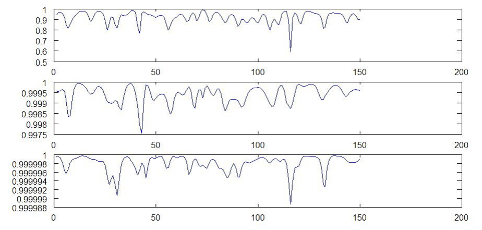
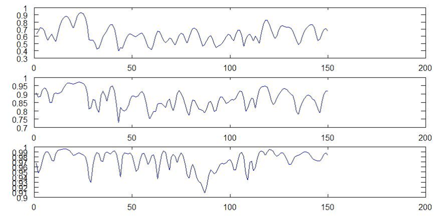
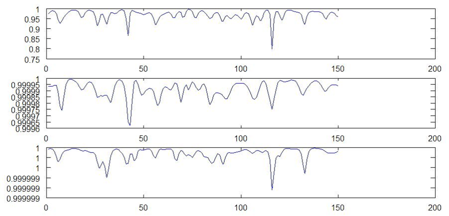
We tested the Cauchy kernel estimator with (3.6) in Example 1 in Experiment 1 and 2 with different $\gamma_{N}$ , the Gaussian kernel ones of Example 2 in Experiment 3 and 4 with different $L_{N}$ .
•

We used Octave ver. 3.2.4, and a Vaio/SONY, Windows 7 64bit OS laptop PC, with processor Intel(R) Core(TM) i3-2310M CPU @2.10GHz 2.10GHz, and RAM 4.00 GB.

All the figures are indicating the results of “dynamical principal component analysis”, where the graphs from the top shows the time evolution of the rate of the biggest, the biggest + the second, and the first three biggest eigenvalues, respectively. Each experiment took about 3 minutes; plausibly fast. We see the similarities between Figure 1 and Figure 2, and between Figure 3 and Figure 4. In these experiments, we should say that the accuracy is not fully appreciated, but we may say that the order of the delta kernel is important to have an accuracy.

Refer to caption — Figure 1. Experiment 1; $\gamma_{N}=(2M_{N}+1)^{-1/2}\approx 0.1796$

References

[1] Liu, N.L., and Mancino, M.E. (2012) “Fourier estimation method applied to forward interest rates”, JSIAM Letters 4, 17-20.
[2] Liu, N.L., and Ngo, H.L. (2014) “Approximation of eigenvalues of spot cross volatility matrix with a view toward principal component analysis”, arXiv:1409.2214 [q-fin.ST].
[3] Malliavin, P. and Mancino, M.E. (2002) “Fourier Series Method for Measurement of Multivariate Volatilities”, Finance and Stochastics , 6, pp.49–61.
[4] Malliavin, P. and Mancino, M.E. (2009) Fourier Transform Method for Nonparametric Estimation of Multivariate Volatility The Annals of Statistics, vol. 37, No. 4, pp.1983–2010.
[5] Mancino, M.E. and Sanfelici, S.: Estimating Covariance via Fourier Method in the Presence of Asynchronous Trading and Microstructure Noise Journal of Financial Econometrics (2011), vol. 9, No. 2, pp.367–408.
[6] Ngo, H.L. and Ogawa, S.: A Central Limit Theorem for the Functional Estimation of the Spot Volatility Monte Carlo Methods and Applications (2009), vol. 15, No. 4, pp.353–380.