Riemannian Multi-Manifold Modeling
Abstract
This paper advocates a novel framework for segmenting a dataset in a Riemannian manifold into clusters lying around low-dimensional submanifolds of . Important examples of , for which the proposed clustering algorithm is computationally efficient, are the sphere, the set of positive definite matrices, and the Grassmannian. The clustering problem with these examples of is already useful for numerous application domains such as action identification in video sequences, dynamic texture clustering, brain fiber segmentation in medical imaging, and clustering of deformed images. The proposed clustering algorithm constructs a data-affinity matrix by thoroughly exploiting the intrinsic geometry and then applies spectral clustering. The intrinsic local geometry is encoded by local sparse coding and more importantly by directional information of local tangent spaces and geodesics. Theoretical guarantees are established for a simplified variant of the algorithm even when the clusters intersect. To avoid complication, these guarantees assume that the underlying submanifolds are geodesic. Extensive validation on synthetic and real data demonstrates the resiliency of the proposed method against deviations from the theoretical model as well as its superior performance over state-of-the-art techniques.
1 Introduction
Many modern data sets are of moderate or high dimension, but manifest intrinsically low-dimensional structures. A natural quantitative framework for studying such common data sets is multi-manifold modeling (MMM) or its special case of hybrid-linear modeling (HLM). In this MMM framework a given dataset is modeled as a union of submanifolds (whereas HLM considers union of subspaces). When proposing a valid algorithm for MMM, one assumes an underlying dataset that can be modeled as mixture of submanifolds and tries to prove under some conditions that the proposed algorithm can cluster the dataset according to the submanifolds. This framework has been extensively studied and applied for datasets embedded in the Euclidean space or the sphere (Arias-Castro et al., 2011; Arias-Castro et al., 2013; Cetingul and Vidal, 2009; Elhamifar and Vidal, 2011; Kushnir et al., 2006; Ho et al., 2013a; Lui, 2012; Wang et al., 2011).
Nevertheless, there is an overwhelming number of application domains, where information is extracted from datasets that lie on Riemannian manifolds, such as the Grassmannian, the sphere, the orthogonal group, or the manifold of symmetric positive (semi)definite [P(S)D] matrices. For example, auto-regressive moving average (ARMA) models are utilized to extract low-rank linear subspaces (points on the Grassmannian) for identifying spatio-temporal dynamics in video sequences (Turaga et al., 2011). Similarly, convolving patches of images by Gabor filters yields covariance matrices (points on the PD manifold) that can capture effectively texture patterns in images (Tou et al., 2009). Nevertheless, current MMM strategies are not sufficiently accurate for handling data in more general Riemannian spaces.
The purpose of this paper is to develop theory and algorithms for the MMM problem in more general Riemannian spaces that are relevant to important applications.
Related Work.
Recent advances in parsimonious data representations and their important implications in dimensionality reduction techniques have effected the development of non-standard spectral-clustering schemes that result in state-of-the-art results in modern applications (Arias-Castro et al., 2013; Chen and Lerman, 2009a; Elhamifar and Vidal, 2009; Goh and Vidal, 2008; Goldberg et al., 2009; Harandi et al., 2013; Liu et al., 2013; Zhang et al., 2012). Such schemes rely on the assumption that data exhibit low-dimensional structures, such as unions of low-dimensional linear subspaces or submanifolds embedded in Euclidean spaces.
Several algorithms for clustering on manifolds are generalizations of well-known schemes developed originally for Euclidean spaces. For example, Gruber and Theis (2006) extended the classical -means algorithm from Euclidean spaces to Grassmannians, and illustrated an application to nonnegative matrix factorization. Tuzel et al. (2005) capitalized on the Riemannian distance of to design an efficient mean-shift (MS) algorithm for multiple 3D rigid motion estimation. Subbarao and Meer (2006), as well as Cetingul and Vidal (2009), extended further the MS algorithm to general analytic manifolds including Grassmannians, Stiefel manifolds, and matrix Lie groups. O’Hara et al. (2011) showed promising results by using the geodesic distance of product manifolds in clustering of human expressions, gestures, and actions in videos. Rathi et al. (2007) solved the image segmentation problem, after recasting it as a matrix clustering problem, via probability distributions on symmetric PD matrices. Goh and Vidal (2008) extended spectral clustering and nonlinear dimensionality reduction techniques to Riemannian manifolds. These previous works are quite successful when the convex hulls of individual clusters are well-separated, but they often fail when clusters intersect or are closely located.
HLM and MMM accommodate low-dimensional data structures by unions of subspaces or submanifolds, respectively, but are restricted to manifolds embedded in either a Euclidean space or the sphere. Many strategies have been suggested for solving the HLM problem, known also as subspace clustering. These strategies include methods inspired by energy minimization (Bradley and Mangasarian, 2000; Ho et al., 2003; Ma et al., 2007; Poling and Lerman, 2014; Tseng, 2000; Zhang et al., 2009; Zhang et al., 2010), algebraic methods (Boult and Brown, 1991; Costeira and Kanade, 1998; Kanatani, 2001; Kanatani, 2002; Ma et al., 2008; Ozay et al., 2010; Vidal et al., 2005), statistical methods (Tipping and Bishop, 1999; Yang et al., 2006), and spectral-type methods with various types of affinities representing subspace-related information (Chen and Lerman, 2009a; Elhamifar and Vidal, 2013; Liu et al., 2013; Yan and Pollefeys, 2006; Zhang et al., 2012). Recent tutorial papers on HLM are Vidal (2011) and Aldroubi (2013). Some theoretical guarantees for particular HLM algorithms appear in (Chen and Lerman, 2009b; Lerman and Zhang, 2011; Soltanolkotabi and Candès, 2012; Soltanolkotabi et al., 2014). There are fewer strategies for the MMM problem, which is also known as manifold clustering. They include higher-order spectral clustering (Arias-Castro et al., 2011), spectral methods based on local PCA (Arias-Castro et al., 2013; Goldberg et al., 2009; Gong et al., 2012; Kushnir et al., 2006; Wang et al., 2011), sparse-coding-based spectral clustering in a Euclidean space (Elhamifar and Vidal, 2011) and its modification to the sphere by Cetingul et al. (2014) (the sparse coding encodes local subspace approximation), energy minimization strategies (Guo et al., 2007), methods based on manifold learning algorithms (Polito and Perona, 2001; Souvenir and Pless, 2005), and methods based on clustering dimension or local density (Barbará and Chen, 2000; Gionis et al., 2005; Haro et al., 2006). Notwithstanding, only higher-order spectral clustering and spectral local PCA are theoretically guaranteed (Arias-Castro et al., 2011; Arias-Castro et al., 2013).
In a different context, Rahman et al. (2005) suggested multiscale strategies for signals taking values in Riemannian manifolds, in particular, the sphere, the orthogonal group, the Grassmannian, and the PD manifold. Even though Rahman et al. (2005) addresses a completely different problem, its basic principle is similar in spirit to ours and can be described as follows. Local analysis is performed in the tangent spaces, where the exponential and logarithm maps are used to transform data between local manifold neighborhoods and local tangent space neighborhoods. Information from all local neighborhoods is then integrated to infer global properties.
Contributions.
Despite the popularity of manifold learning, the associated literature lacks generic schemes for clustering low-dimensional data embedded in non-Euclidean spaces. Furthermore, even in the Euclidean setting only few algorithms for MMM or HLM are theoretically guaranteed. To this end, this paper aims at filling this gap and provides an MMM approach in non-Euclidean setting with some theoretical guarantees even when the clusters intersect. In order to avoid nontrivial theoretical obstacles, the theory assumes that the underlying submanifolds are geodesic and refer to it as multi-geodesic modeling (MGM). Clearly, this modeling paradigm is a direct generalization of HLM from Euclidean spaces to Riemannian manifolds. A more practical and robust variant of the theoretical algorithm is also developed, and its superior performance over state-of-the-art clustering techniques is exhibited by extensive validation on synthetic and real datasets. We remark that in practice we require that the logarithm map of can be computed efficiently and we show that this assumption does not restrict the wide applicability of this work.
We believe that it is possible to extend the theoretical foundations of this work to deal with general submanifolds by using local geodesic submanifolds (in analogy to Arias-Castro et al. (2013)). However, this will significantly increase the complexity of our proof, which is already not simple. Nevertheless, the proposed method directly applies to the more general setting (without theoretical guarantees) since geodesics are only used in local neighborhoods and not globally. Furthermore, our numerical experiments show that the proposed method works well in real practical scenarios that deviate from the theoretical model.
On a more technical level, the paper is distinguished from previous works in multi-manifold modeling in its careful incorporation of “directional information,” e.g., local tangent spaces and geodesics. This is done for two purposes: (i) To distinguish submanifolds at intersections; (ii) to filter out neighboring points that belong to clusters different than the cluster of the query point. In such a way, the proposed algorithm allows for neighborhoods to include points from different clusters, while previous multi-manifold algorithms (e.g., Elhamifar and Vidal (2011)) need careful choice of neighborhood radii to avoid points belonging to other clusters.
2 Theoretical Preliminaries
We formulate the theoretical problem of MGM and review preliminary background of Riemannian geometry, which is necessary to follow this work.
2.1 Multi-Geodesic Modeling (MGM)
MGM assumes that each point in a given dataset lies in the tubular neighborhood of some unknown geodesic submanifold , , of a Riemannian manifold, .11 1 The tubular neighborhood with radius of in (with metric tensor and induced distance ) is . The goal is to cluster the dataset into groups such that points in are associated with the submanifold . Note that if is a Euclidean space, geodesic submanifolds are subspaces and MGM boils down to HLM, or equivalently, subspace clustering (Elhamifar and Vidal, 2009; Vidal, 2011; Zhang et al., 2012).
For theoretical purposes, we assume the following data model, which we refer to as uniform MGM: The data points are i.i.d. sampled w.r.t. the uniform distribution on a fixed tubular neighborhood of . We denote the radius of the tubular neighborhood by and refer to it as the noise level. Figure 1 illustrates data generated from uniform MGM with two underlying submanifolds (.

The MGM problem only serves our theoretical justification. The numerical experiments show that the proposed algorithm works well under a more general MMM setting. Such a setting may include more general submanifolds (not necessarily geodesic), non-uniform sampling and different kinds and levels of noise.
2.2 Basics of Riemannian Geometry
This section reviews basic concepts from Riemannian geometry; for extended and accessible review of the topic we recommend the textbook by do Carmo (1992). Let be a -dimensional Riemannian manifold with a metric tensor . A geodesic between is a curve in whose length is locally minimized among all curves connecting and . Let be the Riemannian distance between and on . If denotes the tangent space of at , then stands for the tangent subspace of a -dimensional geodesic submanifold at . As shown in Figure 2a, is a linear subspace of . The exponential map maps a tangent vector to a point , which provides local coordinates around . By definition, the geodesic submanifold is the image of under (cf., Definition 2). The functional inverse of is the logarithm map from to , which maps to the origin of . Let denote the image of a data point in by the logarithm map at ; that is, .


3 Solutions for the MGM (or MMM) Problem in
We suggest solutions for the MMM problem in with theoretical guarantees supporting one of these solutions when restricting the problem to MGM. Section 3.1 defines two key quantities for quantifying directional information: Estimated local tangent subspaces and geodesic angles. Section 3.2 presents the two solutions and discusses their properties.
3.1 Directional Information
The Estimated Local Tangent Subspace .
Figure 2b demonstrates the main quantity defined here () as well as related concepts and definitions. It assumes a dataset generated by uniform MGM with a single geodesic submanifold . The dataset is thus contained in a tubular neighborhood of a -dimensional geodesic submanifold . Since is geodesic, for any the set of images by the logarithm map is contained in a tubular neighborhood of the -dimensional subspace (possibly with a different radius than ).
Since the true tangent subspace is unknown, an estimation of it, , is needed. Let be the neighborhood of with a fixed radius . Let
| (1) |
Moreover, let denote the local sample covariance matrix of the dataset on , and the spectral norm of , i.e., its maximum eigenvalue. Since is in a tubular neighborhood of a -dimensional subspace, estimates of the intrinsic dimension of the local tangent subspace, which is also the dimension of , can be formed by bottom eigenvalues of (cf., Arias-Castro et al. (2013)). We adopt this strategy of dimension estimation and define the estimated local tangent subspace, , as the span in of the top eigenvectors of . In theory, the number of top eigenvectors is the number of eigenvalues of that exceed for some fixed (see Theorem 1 and its proof for the choice of ). In practice, the number of top eigenvectors is the number of top eigenvalues until the largest gap occurs.
Empirical Geodesic Angles.
Let be the shortest geodesic (global length minimizer) connecting and in . Let be the tangent vector of at . In other words, shows the direction at of the shortest path from to . Given a dataset , the empirical geodesic angle is the elevation angle (cf., (9) of Lerman and Whitehouse (2009)) between the vector and the subspace in the Euclidean space .
3.2 Proposed Solutions
In Section 3.2.1, we propose a theoretical solution for data sampled according to uniform MGM. We start with its basic motivation, then describe the proposed algorithm and at last formulate its theoretical guarantees. In Section 3.2.2, we propose a practical algorithm. At last, Section 3.2.3 discusses the numerical complexity of both algorithms.
3.2.1 Algorithm 1: Theoretical Geodesic Clustering with Tangent information (TGCT)
The proposed solution for the MGM-clustering task applies spectral clustering with carefully chosen weights. Specifically, a similarity graph is constructed whose vertices are data points and whose edges represent the similarity between data points. The challenge is to construct a graph such that two points are locally connected only when they come from the same cluster. This way spectral clustering will recover exactly the underlying clusters.
For the sake of illustration, let us assume only two underlying geodesic submanifolds and . We also assume that the data was sampled from according to uniform MGM. Given a point one wishes to connect to it the points from the same submanifold within a local neighborhood for some . Clearly, it is not realistic to assume that all points in are from the same submanifold of (due to nearness and intersection of clusters as demonstrated in Figures 3a and 3b).
We first assume no intersection at as demonstrated in Figure 3a. In order to be able to identify the points in from the same submanifold of , we use local tangent information at . If belongs to , then the geodesic has a large angle with the tangent space at . On the other hand, if such belongs to , then the geodesic has an angle close to zero. Therefore, thresholding the empirical geodesic angles may become beneficial for eliminating neighboring points belonging to a different submanifold (cf., Figure 3a).


If is at or near the intersection, it is hard to estimate correctly the tangent spaces of each submanifold and the geodesic angles may not be reliable. Instead, one may compare the dimensions of estimated local tangent subspaces. The estimated dimensions of local neighborhoods of data points, which are close to intersections, are larger than the estimated dimensions of local neighborhoods of data points further away from intersections (cf., Figure 3b). The algorithm thus connects to other neighboring points only when their “local dimensions” (linear-algebraic dimension of the estimated local tangent) are the same. In this way, the intersection will not be connected with the other clusters.
The dimension difference criterion, together with the angle filtering procedure, guarantee that there is no false connection between different clusters (the rigorous argument is established in the proof of Theorem 1). We use these two simple ideas and the common spectral-clustering procedure to form the Theoretical Geodesic Clustering with Tangent information (TGCT) in Algorithm 1.
The following theorem asserts that TGCT achieves correct clustering with high probability. Its proof is in Section 5. Its statement relies on the constants and , which are clarified in the proof and depend only on the underlying geometry of the generative model. For simplicity, the theorem assumes that there are only two geodesic submanifolds and that they are of the same dimension. However, it can be extended to geodesic submanifolds of different dimensions.
Theorem 1
Consider two smooth compact -dimensional geodesic submanifolds, and , of a Riemannian manifold and let be a dataset generated according to uniform MGM w.r.t. with noise level . If the positive parameters of the TGCT algorithm, , , and , satisfy the inequalities
| (2) | ||||
then with probability at least , the TGCT algorithm can cluster correctly a sufficiently large subset of , whose relative fraction (over ) has expectation at least .
3.2.2 Algorithm 2: Geodesic Clustering with Tangent information (GCT)
A practical version of the TGCT algorithm, which we refer to as Geodesic Clustering with Tangent information (GCT), is described in Algorithm 2. This is the algorithm implemented for the experiments in Section 4 and its choice of parameters is clarified in Section A.2. GCT differs from TGCT in three different ways. First, hard thresholds in TGCT are replaced by soft ones, which are more flexible. Second, the dimension indicator function is dropped from the affinity matrix . Indeed, numerical experiments indicate that the algorithm works properly without the dimension indicator function, whenever there is only a small portion of points near the intersection. This numerical observation makes sense since the dimension indicator is only used in theory to avoid connecting intersection points to points not in intersection. At last, pairwise distances are replaced by weights resulting from sparsity-cognizant optimization tasks. Sparse coding takes advantage of the low-dimensional structure of submanifolds and produces larger weights for points coming from the same submanifold (Elhamifar and Vidal, 2011).
| (3) |
| (4) |
Algorithm 2 solves a sparse coding task in (3). The penalty used is non-standard since the codes are multiplied by (where in Cetingul et al. (2014), these latter terms are all 1). These weights were chosen to increase the effect of nearby points (in addition to their sparsity). In particular, it avoids sparse representations via far-away points that are unrelated to the local manifold structure (see further explanation in Figure 4). Similarly to Cetingul et al. (2014), the clustering weights in (4) exponentiate the sparse-coding weights.

3.2.3 Computational Complexity of GCT and TGCT
We briefly discuss the computational complexity of GCT and TGCT, while leaving many technical details to Appendices B and C. The computational complexity of GCT is
where bounds the number of nearest neighbors in a neighborhood (typically by the choice of parameters), CR is the cost of computing the Riemannian distances between any two points and CL is the cost of computing the logarithm map of a given point w.r.t. another point. Furthermore, once was computed, CR. The complexity of CL depends on the Riemannian manifold . If , then CL. If is the space of symmetric PD matrices and , then CL=. If is the Grassmannian, and is chosen to be of the same order as the dimension of the subspaces in , then CL=. In all applications of Riemannian multi-manifold modeling we are aware of is known and it is one of these examples. For more general or unknown , estimation of the logarithm map is discussed in Mémoli and Sapiro (2005) (this estimation is rather slow).
It is possible to reduce the total computational cost under some assumptions. In particular, in theory, it is possible to implement TGCT (or more precisely an approximate variant of it) for the sphere or the Grassmannian with computational complexity of order
where is near zero.
4 Numerical Experiments
To assess performance on both synthetic and real datasets, the GCT algorithm is compared with the following algorithms: Sparse manifold clustering (SMC) (Elhamifar and Vidal, 2011; Cetingul et al., 2014), which is adapted here for clustering within a Riemannian manifold and still referred to as SMC, spectral clustering with Riemannian metric (SCR) of Goh and Vidal (2008), and embedded -means (EKM). The three methods and choices of parameters for all four methods are reviewed in Appendix A.2.
The ground truth labeling is given in each experiment. To measure the accuracy of each method, the assigned labels are first permuted to have the maximal match with the ground truth labels. The clustering rate is computed for that permuted labels as follows:
4.1 Experiments with Synthetic Datasets
Six datasets were generated. Dataset I and II are from the Grassmannian , datasets III and IV are from symmetric positive-definite (PD) matrices, and datasets V and VI are from the sphere . Each dataset contains points generated from two “parallel” or intersecting submanifolds (130 points on each) and cropped by white Gaussian noise. The exact constructions are described below.
Datasets I and II
The first two datasets are on the Grassmannian . In dataset I, 130 pairs of subspaces are drawn from the following non-intersecting submanifolds:
where are equidistantly drawn from and the noise vector comprises i.i.d. normal random variables .
In dataset II, 130 pairs of subspaces lie around two intersecting submanifolds as follows:
where are equidistantly drawn from and the noise vector comprises, again, i.i.d. normal random variables .
Datasets III and IV
The next two datasets are contained in the manifold of symmetric PD matrices.
In dataset III, 130 pairs of matrices of two intersecting groups are generated from the model
| (5) | ||||
where is equidistantly drawn from and is a symmetric matrix whose entries are i.i.d. normal random variables with distribution .
In dataset IV, 130 pairs of matrices of two non-intersecting groups are generated from the model
where are equidistantly drawn from respectively and is a symmetric matrix whose entries are i.i.d. normal random variables with distribution .
Datasets V and VI
Two datasets are constructed on the unit sphere of the 3-dimensional Euclidean space. Dataset V comprises of vectors lying around the following two parallel arcs:
where are equidistantly drawn from . To ensure membership in , vectors generated by and are normalized to unit length. On the other hand, dataset VI considers the following two intersecting arcs:
4.1.1 Numerical Results
Each one of the six datasets is generated according to the postulated models above, and the experiment is repeated times. Table 1 shows the average clustering rate for each method. GCT, SMC and SCR are all based on the spectral clustering scheme. However, when a dataset has low-dimensional structures, GCT’s unique procedure of filtering neighboring points ensures that it yields superior performance over the other methods. This is because both SMC and SCR are sensitive to the local scale , and require each neighborhood not to contain points from different groups. This becomes clear by the results on datasets I, IV, and V of non-intersecting submanifolds. SMC only works well in dataset I, where most of the neighborhoods contain only points from the same cluster, while neighborhoods in datasets IV and V often contain points from different ones. Embedded -means generally requires that the intrinsic means of different clusters are located far from each other. Its performance is not as good as GCT when different groups have low-dimensional structures.
| Methods | Set I | Set II | Set III | Set IV | Set V | Set VI |
|---|---|---|---|---|---|---|
| GCT | 1.00 0.00 | 0.98 0.01 | 0.98 0.00 | 0.95 0.01 | 0.98 0.01 | 0.96 0.01 |
| SMC | 0.97 0.04 | 0.66 0.08 | 0.88 0.03 | 0.80 0.02 | 0.55 0.06 | 0.69 0.05 |
| SCR | 0.51 0.00 | 0.66 0.07 | 0.84 0.00 | 0.80 0.00 | 0.50 0.00 | 0.53 0.07 |
| EKM | 0.50 0.00 | 0.50 0.00 | 0.67 0.00 | 0.50 0.00 | 0.50 0.00 | 0.67 0.06 |
4.2 Robustness to Noise and Running Time
Section 4.1 illustrated GCT’s superior performance over the competing SMC, SCR, and EKM on a variety of manifolds. This section further investigates GCT’s robustness to noise and computational cost pertaining to running time. In summary, GCT is shown to be far more robust than SMC in the presence of noise, at the price of a small increase of running time.
4.2.1 Robustness to Noise
The proposed tangent filtering scheme enables GCT to successfully eliminate neighboring points that originate from different groups. As such, it exhibits robustness in the presence of noise and/or whenever different groups are close or even intersecting. On the other hand, SMC appears to be sensitive to noise due to its sole dependence on sparse weights. Figures 5 and 6 demonstrate the performance of GCT, SMC, SCR, and EKM on the Grassmannian and the sphere for various noise levels (standard deviations of Gaussian noise).

The datasets in Figure 5 are generated on the Grassmannian according to the model of dataset II in Section 4.1 but with different noise levels (in Section 4.1 the noise level was ). Both SMC and SCR appear to be volatile over different datasets, with their best performance never exceeding clustering rate. It is worth noticing that EKM shows poor clustering accuracy. On the contrary, GCT exhibits remarkable robustness to noise, achieving clustering rates above even when the standard deviation of the noise approaches .

GCT’s robustness to noise is also demonstrated in Figure 6, where datasets are generated on the unit sphere according to the model of the dataset VI, but with different noise levels. SMC appears to be volatile also in this setting; it collapses when the standard deviation of noise exceeds , since its affinity matrix precludes spectral clustering from identifying eigenvalues with sufficient accuracy (see further explanation on the collapse of SMC at the end of Section A.2).
4.2.2 Running time
This section demonstrates that GCT outperforms SMC at the price of a small increase in computational complexity. Similarly to any other manifold clustering algorithm, computations have to be performed per local neighborhood, where local linear structures are leveraged to increase clustering accuracy. The overall complexity scales quadratically w.r.t. the number of data-points due to the last step of Algorithm 2, which amounts to spectral clustering of the affinity matrix . Both the optimization task of (3) and the computation of a few principal eigenvectors of the covariance matrix in Algorithm 2 do not contribute much to the complexity since operations are performed on a small number of points in the neighborhood . The computational complexity of GCT is detailed in Appendix C. It is also noteworthy that GCT can be fully parallelized since computations per neighborhood are independent. Nevertheless, such a route is not followed in this section.
Compared with SMC, GCT has one additional component: identifying tangent spaces through local covariance matrices—a task that entails local calculation of a few principal eigenvectors. Nevertheless, it is shown in Appendix C.1 that for neighbors it can be calculated with operations.
The ratios of running times between GCT and SMC for all three types of manifolds are illustrated in Table 2. It can be readily verified that the extra step of identifying tangent spaces in GCT increases running time by less than of the one for SMC.
| Running-time ratio | |||
|---|---|---|---|
| GCT/SMC | 1.06 | 1.05 | 1.11 |
Ratios of running times were also investigated for increasing ambient dimensions of the sphere. More precisely, dataset VI of Section 4.1, which lies in , was embedded via a random orthonormal matrix into the unit sphere , where ranged from to . Figure 7 shows the ratios of the running time of GCT over that of SMC as a function of . We observe that the extra cost of computing the eigendecomposition in GCT is mostly less than of SMC, and never exceeds , even when the ambient dimension is as large as .

4.3 Synthetic Brain Fibers Segmentation
Cetingul et al. (2014) cast the problem of segmenting diffusion magnetic resonance imaging (DMRI) data of different fiber tracts as a clustering problem on . The crux of the methodology lies on the transformation of diffusion images, associated with different views of the same object, into orientation distribution functions (ODFs), which are nothing but probability density functions on . The discretized ODF (dODF) is a probability mass function (pmf) , with , that describes the water diffusion pattern at a corresponding location of the object’s image according to the viewing directions . Given and a fixed location, the square-root (SR)dODF is the vector , which lies on the sphere since f is a pmf. In this way, pixels of diffusion images of the same object at a given location are mapped into an element of . Cetingul et al. (2014) assume that each fiber tract is mapped into a submanifold of and thus try to identify different fiber tracts by multi-manifold modeling on .
As suggested in Cetingul et al. (2014), to differentiate pixels with similar diffusion patterns but located far from each other in an image, one has to incorporate pixel spatial information in the segmentation algorithm. Therefore, for GCT, SMC and SCR, the similarity entry of two pixels is modified as
where is the similarity matrix before modification (e.g., for GCT, it is described in Algorithm 2), and is the Euclidean distance between two pixels. For EKM, where no spectral clustering is employed, the dODF is simply augmented with the spatial coordinates of and .


Following Cetingul et al. (2014), we consider here the problem of segmenting or clustering two 2D synthetic fiber tracts in the domain. To generate the fibers, six points are randomly chosen in the colored region of Figure 8a. Two cubic splines passing through and , respectively, are set to be the center of the fibers (cf., red curves in Figure 8b). Fibers are defined as the curved bands around the splines with bandwidth (cf., blue region in Figure 8b).
| Methods | SNR=40 | SNR=30 | SNR=20 | SNR=10 |
|---|---|---|---|---|
| GCT | 0.80 0.12 | 0.82 0.12 | 0.78 0.14 | 0.80 0.13 |
| SMC | 0.73 0.14 | 0.73 0.13 | 0.70 0.13 | 0.67 0.13 |
| SCR | 0.66 0.11 | 0.66 0.11 | 0.68 0.11 | 0.66 0.11 |
| EKM | 0.59 0.08 | 0.58 0.08 | 0.61 0.08 | 0.59 0.08 |

Given a pair of such fibers, the next step is to map each pixel (e.g., both red and blue ones in Figure 8b) to a point (SRdODF) in . To this end, the software code provided by Canales-Rodriguez et al. (2013) is used to generate SRdODFs on , where diffusion images at gradient directions, with baseline image and , are considered. The dimensionality of the generated SRdODFs corresponds to directions. Moreover, Gaussian noise was added in the ODF-generation mechanism, resulting in a signal-to-noise ratio (more details on the construction can be found in Cetingul et al. (2014)). Typical noise levels for real-data brain images are considered: , and (i.e., ).
Once SRdODFs are formed, clustering is carried out on the Riemannian manifold . This in turn provides a segmentation of pixels according to different fiber tracts. A total number of pairs of synthetic brain fibers are randomly generated, and clustering is performed for each pair. Table 3 reports the mean standard deviation of the clustering accuracy rates. Results clearly suggest that GCT outperforms the other three clustering methods. For the case of , Figure 9 plots sample distributions of accuracy rates and shows that GCT demonstrates the highest probability of achieving almost accurate clustering among competing schemes.
4.4 Experiments with Real Data
In this section, GCT performance is assessed on real datasets. Scenarios where data within each cluster have submanifold structures are demonstrated.
4.4.1 Stylized Application: Texture Clustering
We cluster local covariance matrices obtained from various transformations of images of the Brodatz database (Randen, 2014) where the goal is to be able to distinguish between the different images independently of the transformation.
The Brodatz database contains images of pixels with different textures (e.g., brick wall, beach sand, grass) captured under uniform lighting and in frontview position. We apply three simple deformations to these images, which mimic real settings: different lighting conditions, stretching (obtained by shearing) and different viewpoints (obtained by affine transformation). Figure 10 shows sample images in the Brodatz database and their deformations.


Tou et al. (2009) show that region covariances generated by Gabor filters effectively represent texture patterns in a region (patch). Given a patch of size , a Gabor filter of size 1111 with 8 parameters is used to extract 2,500 feature vectors of length 8. This set of feature vectors is then used to compute an 88 covariance matrix for the specific patch.
Three clustering tests, one for each type of deformation, are carried out. In each test, 300 transformed patches are generated equally from 3 different textures and the region covariance is computed for each patch. Then clustering algorithms are applied on the dataset of 300 region covariances belonging to 3 texture patterns. The way to generate transformed patches is described below.
I. Lighting transformation:
A single lighting transformation (demonstrated in Figure 10) is applied to three randomly drawn images from the Brodatz database and 100 patches of size 6060 are randomly picked from each of the 3 transformed images.
II. Horizontal shearing:
Three randomly drawn images are horizontally sheared by 100 different angles to get 3 sequences of 100 shifted images. From each shifted image, a patch of size 6060 is randomly picked.
III. Affine transformation:
Three randomly drawn images are affine transformed to create 3 sequences of 100 affine-transformed images. From each transformed image, a patch of size 6060 is randomly picked.
Figure 11 plots the projection of the embedded datasets generated by the above procedure onto their top three principal components (the embedding to Euclidean spaces is done by direct vectorization of the covariance matrices). The submanifold structure in each cluster can be easily observed.
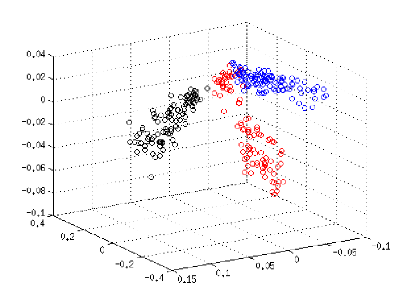
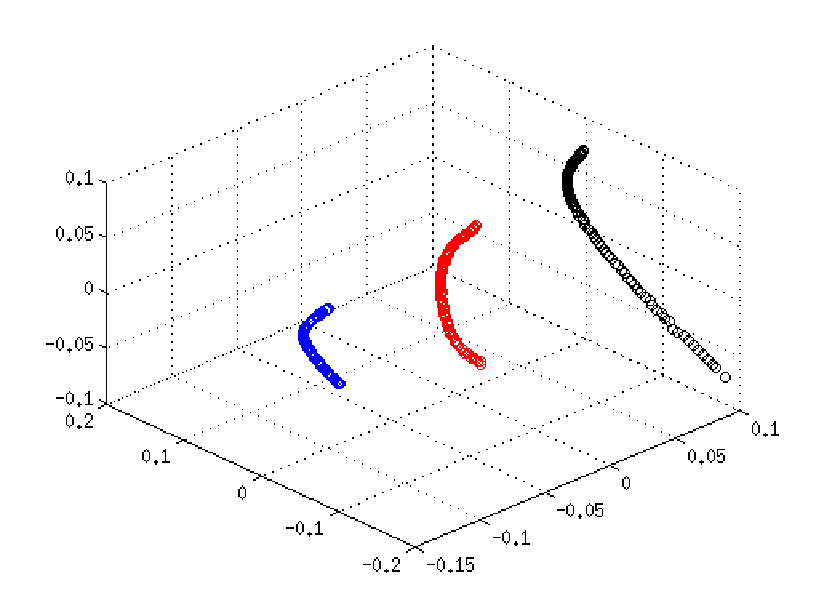
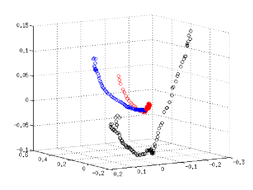
The procedure of generating the data is repeated times for each type of transformation. GCT as well as the other three clustering methods are applied to these datasets, and the average clustering rates are reported in Table 4. GCT exhibits the best performance for all datasets and for all types of transforms.
| Methods | GCT | SMC | SCR | EKM |
|---|---|---|---|---|
| Lighting transformation | 0.73 | 0.53 | 0.68 | 0.67 |
| Horizontal shifting | 0.95 | 0.61 | 0.85 | 0.76 |
| Affine tranformation | 0.83 | 0.53 | 0.82 | 0.76 |
4.4.2 Clustering Dynamic Patterns.
Spatio-temporal data such as dynamic textures and videos of human actions can often be approximated by linear dynamical models (Doretto et al., 2003; Turaga et al., 2011). In particular, by leveraging the auto-regressive and moving average (ARMA) model, we experiment here with two spatio-temporal databases: Dyntex++ and Ballet. Following Turaga et al. (2011), we employ the ARMA model to associate local spatio-temporal patches with linear subspaces of the same dimension. We then apply manifold clustering on the Grassmannian in order to distinguish between different textures and actions in the Dyntex++ and Ballet database respectively.
ARMA Model.
The premise of ARMA modeling is based on the assumption that the spatio-temporal dataset under study is governed by a small number of latent variables whose temporal variations obey a linear rule. More specifically, if is the observation vector at time (in our case, it is the vectorized image frame of a video sequence), then
| (6) | |||
where , , is the vector of latent variables, is the observation matrix, is the transition matrix, and and are i.i.d. sampled vector-values r.vs. obeying the Gaussian distributions and , respectively.
We next explain the idea of Turaga et al. (2011) to associate subspaces with spatio-temporal data. Given data , the ARMA parameters and can be estimated according to the procedure in Turaga et al. (2011). Moreover, by arbitrarily choosing , it can be verified that for any ,
We then set , which is known as the th order observability matrix. If the observability matrix is of full column rank, which was the case in all of the conducted experiments, the column space of is a -dimensional linear subspace of . In other words, the ARMA model estimated from data , , gives rise to a point on the Grassmannian . For a fixed dataset , different choices of , s.t. , and several local regions within the image give rise to different estimates of and and thus to different points in .
Dynamic textures.
The Dyntex++ database (Ghanem and Ahuja, 2010) contains dynamic textures videos of size , which are divided into categories. It is a hard-to-cluster database due to its low resolution. Three videos were randomly chosen, each one from a distinct category from the available ones.
Per video sequence, patches of size are randomly chosen. Each frame of the patch is vectorized resulting into patches of size . To reduce the size to , a (Gaussian) random (linear) projection operator is applied to each patch. As a result, each patch is reduced to the set . We fix and and use each such set to estimate the underlying ARMA model. Consequently, points on are generated, per video category.
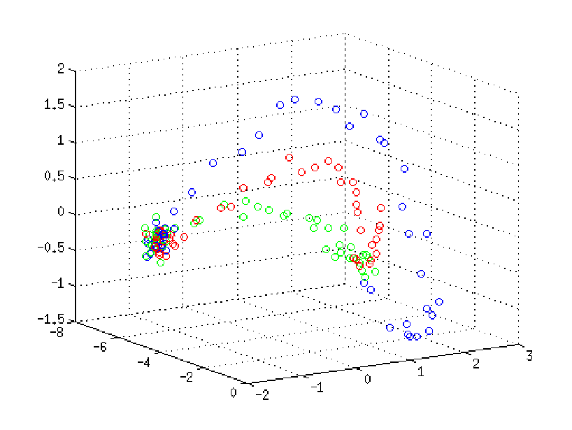
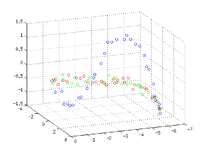
We expect that points in of the same cluster lie near a submanifold of . This is due to the repeated pattern of textures in space and time (they often look like a shifted version of each other in space and time). To visualize the submanifold structure, we isometrically embedded into a Euclidean space (Basri et al., 2011), so that subspaces are mapped to Euclidean points. We then projected the latter points on their top 3 principal components. Figure 13a demonstrates this projection as well as the submanifold structure within each cluster.
Ballet database.
The Ballet database (Wang and Mori, 2009) contains videos of actions from a ballet instruction DVD. The frames of all videos are of size and their lengths vary and are larger than 100. Different performers have different attire and speed. Three videos, each one associated with a different action, were randomly chosen.

Spatio-temporal patches are generated by selecting consecutive frames of size from each one of the following overlapping time intervals: , , , …, . In this way, for each of the three videos, 31 spatio-temporal patches of size are generated. As in the case of the Dyntex++ database, video patches are vectorized and downsized to spatio-temporal patches of size . Following the previous ARMA modeling approach, we set and and associate each such patch with a subspace in . Consequently, 93 subspaces (31 per cluster) in the Grassmannian are generated. Figure 13b visualizes the 3D representation of the subspaces created from three random videos. Their intersection represents still motion.
The procedure described above (for generating data by randomly choosing 3 videos from the Dyntex++ and Ballet databases and applying clustering methods on ) is repeated times. The average clustering accuracy rates are reported in Table 5. GCT achieves the highest rates on both datasets.
| Methods | GCT | SMC | SCR | EKM |
|---|---|---|---|---|
| Dyntex++ | 0.85 | 0.69 | 0.77 | 0.42 |
| Ballet | 0.81 | 0.76 | 0.68 | 0.47 |
5 Proof of Theorem 1
The idea of the proof is as follows. After excluding points sampled near the possibly nonempty intersection of submanifolds, we form a graph whose vertices are the points of the remaining set and whose edges are determined by . The proof then establishes that the resulting graph has two connected components, which correspond to the two different submanifolds and . Spectral clustering can exactly cluster such a graph with appropriate choice of its tuning parameter , which can be specified by self-tuning mechanism (Zelnik-Manor and Perona, 2004). This claim follows from Ng et al. (2001) and its unpublished supplemental material.
The basic strategy of the proof and its organization are described as follows. Section 5.1 presents additional notation used in the proof. Section 5.2 reminds the reader the underlying model of the proof (with some additional details). Section 5.3 eliminates undesirable events of negligible probability (it clarifies the term in the statement of the theorem).
The rest of the proof (described in Sections 5.4-5.8) is briefly sketched as follows. For simplicity, we first assume no noise, i.e., . We define a “sufficiently large” set (and its subsets and ) by the following formula (which uses the notation and ):
| (7) |
In the first part of the proof (see Section 5.4), we show that the graphs of and (with weights ) are respectively connected. If we can show that the graphs of and are disconnected from each other, then the proof can be concluded. To this end, the subsequent auxiliary sets and will be instrumental in the proof. We fix a constant (to be specified later in (34)), which depends on , and the angles of intersection of and , and define
| (8) |
We will verify that and . In fact, it will be a consequence of the second part of the proof. This part shows that the graph of is disconnected from the graph of as well as graph of . Therefore, and cannot be connected via points in . At last, we show that they also cannot be connected within . That is, we show in the third part of the proof (Section 5.6) that the graphs of and are disconnected from each other. These three parts imply that the graphs of and form two connected components within . By definition, and are identified with and respectively. To conclude the proof (for the noiseless case), we estimate the measure of the set , which was excluded. More precisely, we consider the measure of the set , which we define as follows
| (9) |
This measure estimate and the conclusion of the proof (to the noiseless case) are established in Section 5.7. Section 5.8 discusses the generalization of the proof to the noisy case.
Various ideas of the proof follow Arias-Castro et al. (2013), which considered multi-manifold modeling in Euclidean spaces. Some of the arguments in the proof of Arias-Castro et al. (2013) even apply to general metric spaces, in particular, to Riemannian manifolds. We thus tried to maintain the notation of Arias-Castro et al. (2013).
However, the algorithm construction and the main theoretical analysis of Arias-Castro et al. (2013) are valid only when the dataset lies in a Euclidean space and it is nontrivial to extend them to a Riemannian manifold. Indeed, the basic idea of Arias-Castro et al. (2013) is to compare local covariance matrices and use this comparison to infer the relation between the corresponding data points, over which those matrices were generated. However, comparing local covariance matrices in the case where the ambient space is a Riemannian manifold is not straightforward as in Euclidean spaces. This is due to the fact that local covariance matrices are computed at different tangent spaces with different coordinate systems. Instead we show that it is sufficient to compare the “local directional information” (i.e., empirical geodesic angles) and “local dimension”. Both of these quantities are derived from the local covariance matrices. However, due to the nonlinear mapping to the tangent spaces, which distorts the uniform assumption within the ambient space, care must be taken in using the inverse nonlinear map, i.e., the logarithm map.
5.1 Notation
We provide additional notation to the one in Section 2.2. Readers are referred to do Carmo (1992) for a complete introduction to Riemannian geometry.
Let and denote the -neighborhoods of and in and respectively. They are related by the exponential map, , as follows: . We refer to the coordinates obtained in the tangent space by the exponential map as normal coordinates. Using normal coordinates, is endowed with the Riemannian metric and measure . On the other hand, the tangent space can also be identified with by choosing an orthonormal basis. This provides Euclidean metric and measure on , in particular, on . There is a simple relation between and (do Carmo, 1992):
| (10) |
Figure 14 highlights the difference between and . It shows the tangent space of the north pole, , of and the straight blue line connecting and in ; it is the shortest path w.r.t. . On the other hand, the shortest path w.r.t. is clearly the equator (the geodesic connecting and ), which is the black arc on ; it is different than the blue line. In fact, only lines in connecting the origin and other points on correspond to geodesics on for a general metric. As a consequence, the measures and induced by and are also different.

Given a submanifold (or a -tubular neighborhood of ), the metric tensor on (or ) inherited from induces a measure on (or ), which is called the uniform measure on (or ). For simplicity we assume throughout most of the proof that and thus mainly discuss the measure on . In Section 5.8 we generalize the proof to the noisy case and thus discuss on . The push-forward measure of by is a measure on , which is again denoted by . By definition, the support of the push-forward measure is , which is a submanifold of . The Euclidean metric similarly induces another measure , which is supported on .
For a measure on and a subset of positive such measure, the expected covariance matrix is defined by
| (11) |
For the two compact submanifolds of the model, and , we denote and define the following two measures w.r.t. S: and . The covariance matrices w.r.t. and are denoted by and , respectively. For simplicity, when , we denote them by and . For , we denote them by and .
If a dataset is given, let denote the sample covariance of the data on and denote the sample covariance of the data on . Let denote the minimal nonzero principal angle between the subspaces 22 2 We only use when there is a nonzero principal angle. It is thus well-defined. and let
| (12) |
For , let denote the largest principal angle between and and let
| (13) |
Recall that the notation
means that there is a constant independent of such that
| (14) |
If and are matrices, then (14) applies to their entries. If , we denote by the tangent vector of at (it was denoted by in Section 2.2). We denote the empirical geodesic angle between and by (where for data points , , ). Lastly, for a matrix , stands for the th largest eigenvalue of .
5.2 A Generative Multi-Geodesic Model
We review in more details the generative model for two geodesic submanifolds (see Section 2.1). We first state the definition of geodesic submanifolds.
Definition 2
For a Riemannian manifold , a submanifold is called a geodesic submanifold if , the shortest geodesic connecting and in is also contained in .
Let , be two compact geodesic submanifolds of dimension in a Riemannian manifold and recall that . Let , and denote -tubular neighborhoods of , and respectively. For example, , where . The dataset of size is i.i.d. sampled from the normalized version of (by ) on . We recall the notation: and . Fixing a point , then is i.i.d. sampled from the normalized push-forward on .
5.3 Local Concentration with High Probability
We verify here the concentration of the local covariance matrices and the existence of sufficiently large samples in local neighborhoods from the same submanifold. We follow Arias-Castro et al. (2013)33 3 For simplicity, we set the parameter of Arias-Castro et al. (2013) to be equal to and define on the probability space (i.e., ), the following events and :
| (15) |
| (16) |
where and are specified in Arias-Castro et al. (2013) ( depends on and (defined in (12)) and depends on the covering number of ) and is the sample covariance of images on . We note that is the set of datasets of samples, where each dataset satisfies the following condition: for any point in ( is fixed), there are enough samples that also belong to (their fraction is proportional to ). The set is the set of datasets of samples with sufficient concentration of local covariance matrices. The following theorem of Arias-Castro et al. (2013, page 35) ensures that the event is large. It uses the constant and an absolute constant .
Theorem 3
Let . Then,
In view of this theorem, we assume in the rest of the proof that
| (17) |
5.4 Ensuring Connectedness of and
The following proposition establishes WLOG the connectedness of the graph of the set (defined in (7)). It uses a constant , which is clarified in the proof and depends on geometric properties of and and their angle of intersection.
Proposition 4
There exists a constant such that if
| (18) |
then the graph with nodes at and edges given by is connected.
5.4.1 Proof of Proposition 4
Three different constants , and appear in the proof. As clarified below, they depend on geometric properties of and and their angle of intersection. The constant is then determined by these constants as follows: .
The proof is divided into three parts. The first one shows that for all in if . The second one shows that for all in if . The last one uses an argument of Arias-Castro et al. (2013, page 38). It claims that the graph with nodes at and weights given by the indicator function is connected if .
Part I:
We prove the following lemma, which clearly implies that for .
Lemma 5
There exists a constant such that if , and , then
| (19) |
Proof Recall that denotes the sample covariance of the transformed data . We denote and note that
| (20) | ||||
The first and third equalities of (20) follow from the definition of the expected covariance. The second equality of (20) follows from (10) and the fact that . A slight generalization of Lemma 11 of Arias-Castro et al. (2013) implies that
| (21) |
where is the orthogonal projector onto in . Equation (20) and (21) imply that
| (22) |
where is a constant depending on the Riemannian metric (arising due to (10)). Using this constant , we define
| (23) |
We note that . Combining this observation with the following two assumptions: and , we conclude that .
Combining the triangle inequality, (17), (22) and the fact that , we conclude that
| (24) |
The application of both Weyl’s inequality (Stewart and Sun, 1990) and (24) results in the following lower bound of and upper bound of :
| (25) |
It follows from (23), (25) and elementary algebraic manipulations that
| (26) | ||||
Equation (19) thus follows from (26) and the thresholding of eigenvalues by in Algorithm 1.
Part II:
Next, we prove that if .
Lemma 6
There exists a constant such that if and
| (27) |
then .
Proof We define
| (28) |
where is the constant introduced in (22). We show that for :
| (29) |
which immediately implies the lemma.
In order to prove (29), we first apply the Davis-Kahan Theorem (Davis and Kahan, 1970) and (19) and then apply (24) to obtain the following bound on the distance between the subspaces and (which are spanned by the top eigenvectors of and , respectively; this observation uses (19)):
| (30) |
We remark that in applying the Davis-Kahan Theorem we made use of the following basic calculation of , the th spectral gap of : .
Next, we recall that denotes the largest principal angle between and . We note that Lemma 15 of Arias-Castro et al. (2013) (whose application requires (19)), (30), (28) and Jordan’s inequality (lower bounding the function by ) imply that
| (31) |
Since is the angle between and , (29) follows from (31). We can then conclude that if , then for all in .
Part III:
By the construction of the affinity matrix and Lemmata 5 and 6, the connectivity between points is solely determined by the indicator function . It is obvious that if then the graph with nodes in and weights is connected (this can be done by finite covering of with balls of radius ). It follows from Arias-Castro et al. (2013, pages 38-39) that the graph with nodes in is also connected if
| (32) |
There is one component in the argument of Arias-Castro et al. (2013, page 38) that requires careful adaptation to the Riemannian case. It is related to the determination of the constant . This constant is set to be (see Arias-Castro et al. (2013, page 39)). In the Euclidean case, is guaranteed by Lemma 18 of Arias-Castro et al. (2013). The adaptation of this Lemma to the Riemannian case can be stated in the following lemma (it uses , which was defined in (12)).
Lemma 7
Let be a Riemannian manifold and , be two compact geodesic submanifolds of dimension such that . Then there is a constant such that
5.5 Disconnectedness Between and (or )
We show here that the points in (where is defined in (8)) are not connected to the points of . In Section 5.4, we showed that the estimated dimensions of local neighborhoods of points in equal . In this section, we show that the estimated dimensions of local neighborhoods of points in are larger than . Since is a multiplicative term of , we conclude that is disconnected from . The following main proposition of this section implies that WLOG the estimated tangent dimension at is at least (it uses the angle defined in (13)).
Proposition 8
There exists a constant depending only on and such that if ,
| (33) |
| (34) |
and
| (35) |
then
Proof Let us first sketch the idea of the proof. It is easier to estimate the local covariance matrices when the two manifolds are subspaces (see Lemma 21 of Arias-Castro et al. (2013)). However, for , the logarithm map of into does not result in two subspaces (see Figure 15). On the other hand, for , the projection of onto , the logarithm map of into results in two subspaces, where the local covariance can be estimated more easily. Some difficulties arise due to the application of the logarithm map and the change of tangent spaces. In particular, the ball becomes irregular in the domain .
We recall that and . We arbitrarily fix such that . We note that Lemma 7 implies that
| (36) |
Let
where if argmin is not uniquely defined, then is arbitrarily chosen among all minimizers. It follows from (36) that and from this and the triangle inequality, it follows that
| (37) |
Recall that and denote the normal coordinate charts around and respectively (see Figure 15); it is sufficient to restrict them to and respectively. When using the chart , and correspond to two subspaces in , which we denote by and respectively. On the other hand, when using the chart , corresponds to a manifold in , whereas still corresponds to a subspace.

It follows from (37) and the invertibility of that the composition map embeds into as shown in Figure 15. Recall that denotes the sample covariance of the data in and denotes the sample covariance of the data in . Using the notation for the set of orthogonal matrices, we claim that
| (38) |
We estimate as follows. Let and (see Figure 16), where is the -ball with center in , which uses the Euclidean distance .

The rest of the proof requires the following two technical observations
| (39) |
and
| (40) |
We prove (39) in Appendix D.3. The first equality of (40) follows from the definition of the expected covariance (see (11)), (10) and the fact that . The second equality of (40) follows from the definition of the expected covariance (see (11)), (39) and the fact that .
The combination of (41), Weyl’s inequality (Stewart and Sun, 1990) for and , and the fact that and have the same eigenvalues implies that
| (42) |
Notice that by definition. Applying (42) and Lemma 21 of Arias-Castro et al. (2013) to , where is replaced by and proper scaling is used, results in
| (43) |
We remark that the second inequality of (43) is derived by applying the bound: . In order to satisfy , we require that
| (44) |
Since , we replace with in the numerator of (44) and with in the denominator of (44) and slightly simplify the inequality to obtain the following stronger requirement:
| (45) |
Finally, setting
| (46) |
we can rewrite (45) as follows
| (47) |
We immediately conclude (47) (and consequently the lemma) from (34) and (35).
We end this section with an immediate corollary of Proposition 8, which is crucial in order to follow the proof.
Corollary 9
The following relations are satisfied:
5.6 The Disconnectedness of and
We show here that the graphs with nodes at and are disconnected. The idea is to show that the function (and thus the weight ) is zero between two points in and for appropriate choice of constants. This and Proposition 8 imply that the graphs associated with and are disconnected. We first establish a lower bound on the empirical geodesic angle in Lemma 10 and then conclude that there is no direct connection between the sets and in Corollary 11.
Lemma 10
There exist constants and such that if , ,
| (48) |
| (49) |
then the angle between the estimated tangent subspace and the line segment , which connects the origin and (the image of by ) in is bounded below as follows:
| (50) |
Proof The proof develops various geometric estimates that eventually conclude (50). Let
where is defined with respect to the normal coordinate chart in (see Figure 17).

We note that by definition is the projection of onto and thus
| (51) |
Combining (51) with the fact that and are the same on lines through the origin in and then applying (48), we obtain that
| (52) |
Furthermore, combining the following two facts: is a minimizer of and , we obtain that
| (53) |
We prove in Appendix D.4 that there exists a constant , which depends only on the Riemannian manifold , such that
| (54) |
Applying (54) (with ) first and (53) next we obtain that
| (55) |
and consequently
| (56) |
It follows from (49) and (56) that
| (57) |
Inequalities (58) and (59) are verified in Appendices D.5 and D.6 respectively, where we also carefully analyze how the constant depends on the underlying Riemannian manifold (see (102)). Combining (57), (58) and (59), we conclude (50) by letting .
The desired disconnectedness of and immediately follows from Lemma 10 in the following way:
Corollary 11
The graphs with nodes at and respectively and weights in are disconnected if the angle threshold is chosen such that
| (60) |
and the distance threshold satisfies (49).
Proof
When and satisfy (60)
and (49) respectively, Lemma 10 implies
that if and , then
. In
other words, there is no direct connection between and through
. On the other hand, Lemma 5 and
Proposition 8 imply that and cannot be
connected through points in (since points in and
have different local estimated dimensions). We thus conclude that and
are disconnected.
5.7 Conclusion of Theorem 1 for the Noiseless Multi-Geodesic Model
Due to Theorem 3 we replace with and obtain a statement for with probability at least . Proposition 4 and Corollary 11 imply that (with probability at least ) has two connected components. They require that the parameters of TGCT satisfy (18), (49) and (60). Additional requirement is specified in (33) (in Proposition 8 which implies Corollary 11). We also note that the requirement , which also appears in some of the auxiliary lemmata, follows from (18), (33) and the fact that and . These requirements, i.e., (18), (33), (49) and (60), are sufficient and equivalent to (2) when .
Next, we explain why one can choose parameters that satisfy these requirements at the end of this section. The only problem is to make sure that the last inequality of (2) (equivalently, (60)) is satisfied. Given a sufficiently small satisfying (18), we let for some fixed . The RHS of (60) tends to as and approach zero. We note that the lower bound of is . Therefore, if and are sufficiently small so that is lower than the RHS of (60) and , then can be chosen from the interval .
In order to conclude the proof in this case we upper bound the expected portion of points , where and denote he cardinality of and respectively. For this purpose we use the set , which was defined in (9) in the following way:
| (61) | ||||
The first equality of (61) follows from the fact that the dataset is i.i.d. sampled from . The second inequality of (61) follows from Lemma 7. The last one follows from Theorem 1.3 in Gray (1982), where is a constant depending only on the geometry of the underlying generative model (e.g., the mean curvature and volume of ).
5.8 Conclusion of Theorem 1 for the Noisy Multi-Geodesic Model
The above analysis also applies when the generative multi-geodesic model has noise level and is sufficiently smaller than , that is,
| (62) |
where . Indeed, in this case the estimates of tangent spaces and geodesics are sufficiently close to the estimates without noise. The only difference is that the last bound in (61) has to be replaced with . This requires though a sufficiently small noise level (set by ). Precise bound on is not trivial. Furthermore, the analysis employed here is not optimal. We can thus only claim in theory robustness to very small levels of noise, whereas robustness to higher levels of noise is studied in the experiments.
6 Conclusions
Aiming at efficiently organizing data embedded in a non-Euclidean space according to low-dimensional structures, the present paper studied multi-manifold modeling in such spaces. The paper solves this clustering (or modeling) problem by proposing the novel GCT algorithm. GCT thoroughly exploits the geometry of the data to build a similarity matrix that can effectively cluster the data (via spectral clustering) even when the underlying submanifolds intersect or have different dimensions. In particular, it introduces the novel idea in non-Euclidean multi-manifold modeling of using directional information from local tangent spaces to avoid neighboring points of clusters different than that of the query point. Theoretical guarantees for successful clustering were established for a variant of GCT, namely TGCT for the MGM setting, which is a non-Euclidean generalization of the widely-used framework of hybrid-linear modeling. Unlike TGCT, GCT combined directional information from local tangent spaces with sparse coding, which aims to improve the clustering result by the use of more succinct representations of the underlying low-dimensional structures and by increasing robustness to corruption. Geodesic information is only used locally and thus in practice the algorithm can fit well in practice to MMM and not MGM. Validated against state-of-the-art existing methods for the non-Euclidean setting, GCT exhibited notable performance in clustering accuracy. More specifically, the paper tested GCT on synthetic and real data of deformed images clustering, action identification in video sequences, brain fiber segmentation in medical imaging and dynamic texture clustering.
7 Acknowledgments
This work was supported by the Digital Technology Initiative, a seed grant program of the Digital Technology Center, University of Minnesota, NSF awards DMS-09-56072, DMS-14-18386 and Eager-13-43860, the University of Minnesota Doctoral Dissertation Fellowship Program, and the Feinberg Foundation Visiting Faculty Program Fellowship of the Weizmann Institute of Science.
Appendix A Competing Clustering Algorithms and Their Implementation Details
Section A.1 reviews the competing methods of GCT (in the Riemannian setting) and Section A.2 describes the implementation of both GCT and the competing algorithms, in particular, the choice of all parameters.
A.1 Review of Competing Algorithms
The first competing algorithm is sparse manifold clustering (SMC). This algorithm was first suggested by Elhamifar and Vidal (2011) for clustering submanifolds embedded in Euclidean spaces and later modified by Cetingul et al. (2014) for clustering submanifolds of the sphere. We adapt it to the current setting of clustering submanifolds of a Riemannian manifold and still refer to it as SMC. Its basic idea is as follows: For each data-point , a local neighborhood is mapped to the tangent space by the logarithm map and a sparse coding task is solved in to provide weights for the spectral-clustering similarity matrix.
The second competing algorithm is spectral clustering with Riemannian metric (SCR) by Goh and Vidal (2008). It applies spectral clustering with the weight matrix whose entries are (see page 4 of Goh and Vidal (2008)). That is, it replaces the usual Euclidean metric in standard spectral clustering with the Riemannian one.
The third competing scheme is the embedded K-means. It embeds the given dataset, which lies on a Riemannian manifold, into a Euclidean spaces (as explained next) and then applies the classical K-means to the embedded dataset. In the experiments, Grassmannian manifolds are embedded by a well-known isometric embedding into Euclidean space (Basri et al., 2011); the manifolds of symmetric PD matrices are embedded by vectorizing their elements into elements of ; and data in the sphere is already embedded in .
A.2 Implementation Details for All Algorithms
GCT follows the scheme of Algorithm 2. For all algorithms, the number of clusters was known in all experiments The input parameters of GCT are set as follows: The neighborhood radius at a point is chosen to be the average distance of to its th nearest point over all , where ; the distance and angle thresholds and are set to in all experiments (we did not notice a big difference of the results when their values are changed). The dimension of the local tangent space is determined by the largest gap of eigenvalues of each local covariance matrix (more precisely, it is the number of eigenvalues until this gap).
Since there are no online available codes for SMC, SCR and EKM, we wrote our own implementations and will post them (as well as our implementation of GCT) on the supplemental webpage when the paper is accepted for publication. The spectral clustering code in GCT, SMC and SCR, as well as the -means code in EKM are taken from the implementations of Nikvand (2013). To make a faithful comparison, the input parameter of SMC is the same as GCT (in particular, we use the radius of neighborhood and not the number of neighbors). SMC also implicitly sets . There are no other parameters for SMC. We remark that Elhamifar and Vidal (2011) formed the weight matrix as follows: , where and are the sparse coefficients. However, this weight was unstable in some experiments and above a certain level of noise SMC often collapsed in some of the random repetition of the experiments. In such cases, we used instead (for all repetitive experiments for the same data set) the weights suggested in Cetingul et al. (2014) (which are similar to the ones of GCT). In the case of no collapse with the former weights, we tried both weights and noticed that the weights always yielded more accurate results for SMC; we thus used them then even though they can give an advantage over GCT, which uses exponential weights. Overall, the weight was used in the synthetic datasets II-VI of Section 4.1. The exponential weight was used in the rest of the experiments, that is, in synthetic dataset I and in the real or stylized applications. It was also used for dataset VI in Figure 6 under noise levels mostly higher than the noise level used in Section 4.1. The collapse phenomenon is evident in Figure 6 for noise levels above .
The SCR algorithm has only one parameter which is set to 1 (similarly to the analogous parameter of GCT). EKM has no input parameters.
Appendix B Computation of Logarithm Maps and Distances
We discuss the complexity of computing logarithm maps for Grassmannians, symmetric PD matrices and spheres. We remark though that it is possible to compute the logarithm maps for data sampled from more general Riemannian manifolds and without knowledge of the manifold, but at a significantly slower rate (Mémoli and Sapiro, 2005). We also show that once the logarithm map is computed, then in all these cases the computation of the geodesic distances is of lower or equal order.
A fast way to compute the logarithm map of the Grassmannian (whose dimension is ) is provided in Gallivan et al. (2003). It requires a matrix , with orthogonal columns, and a orthonormal matrix for each subspace, where the subspace is spanned by the columns of , with comprising the first columns of . Given two pairs () and (,) for two subspaces, one needs to compute . This computation, which is clarified in Gallivan et al. (2003), includes the singular value decomposition of and . In total, the complexity is , or equivalently, (since ).
For the set of symmetric PD matrices (whose dimension is ), Ho et al. (2013b) computes the logarithm of any such matrices and by first finding the Cholesky decomposition and then computing , where the latter is the matrix logarithm. The complexities of all major operations (i.e., Cholesky decomposition, the matrix logarithm and the matrix multiplication) are . Therefore, the total complexity is also of order , or equivalently, (since the dimension of the set of symmetric PD matrices is ).
The formula for finding the logarithm map on is (see Cetingul et al. (2014))
where is the (Euclidean) dot-vector product. Since it involves inner products and basic operations (also coordinatewise), it takes operations to compute it.
For , . Once we have the image (which is a vector in the tangent space), the Riemannian distance is computed as the Euclidean norm of the image vector, which involves a computation of order . Since the algorithm already computes the logarithm maps, the additional cost for computing the geodesic distances are of lower order than the logarithm maps in all 3 cases.
Appendix C Computational complexity of GCT and TGCT
The computational complexity of GCT is examined per data-point . It involves the computation of Riemannian distances and the logarithm map, which depends on the Riemannian manifold (see estimates in Section B). The complexity of computing the Riemannian distance between and and the logarithm map for w.r.t. are denoted by CR and CL respectively (their computational complexity for the cases of the sphere, Grassmannian and PD matrices were discussed in Appendix B). A major part of GCT occurs in the -neighborhood of (WLOG), where was defined as the average distance to the th nearest point from the associated data-point. To facilitate the analysis of computational complexity, we use instead of the parameter of -nearest-neighbors (-NN) around . Due to the choice of , we assume that .
The complexity for computing the -NN of is , where refers to the complexity of computing distances, and refers to the effort of identifying the smallest ones. The second step of Algorithm 2 is to solve the sparse optimization task in (3). Notice that due to , only the inner products of data-points are necessary to form the loss function in (3), which entails a complexity of order . Given that only -NN are involved in (3) and that their inner products are required to form the loss, (3) is a small scale convex optimization task that can be solved efficiently by any off-the-shelf solver such as the popular alternating direction method of multipliers (Glowinski and Marrocco, 1975; Gabay and Mercier, 1976) or the Douglas-Rachford algorithm (Bauschke and Combettes, 2011). The third step of Algorithm 2 is to find the top eigenvectors of the sample covariance matrix defined by the neighbors of . As shown in Section C.1 below the complexity of this step is . Finally, to compute geodesic angles, operations are necessary. Considering all data-points, the total complexity for the main loop of GCT is . After the main loop, spectral clustering is invoked on the affinity matrix . The main computational burden is to identify eigenvectors of an matrix, which entails complexity of order ( is the number of clusters). In summary, the complexity of GCT is .
Note that in TGCT, the weights of non-neighboring points are set equal to zero, and geodesic angles are computed only for neighboring points, reducing thus the complexity of this step to . Moreover, the affinity matrix is sparse in TGCT, effecting thus a potential decrease in the complexity of spectral clustering to the order of6 (Knyazev, 2001; Kushnir et al., 2010). Therefore, TGCT’s complexity becomes . The only step that contributes to in TGCT comes from -NN. This complexity can be reduced by approximate nearest search. For example, for both the Sphere and the Grassmannian, Wang et al. (2013) established an algorithm for approximate nearest neighbor search, where is a sufficiently small parameter. Therefore the total complexity of TGCT for these special cases can be of order (this includes also the preprocessing for the approximate nearest neighbors algorithm).
C.1 An Algebraic Trick for Fast Computation of the Tangent Subspace
Consider the data matrix at a specific neighborhood with points. We need to identify a few principal eigenvectors of the covariance matrix . One can avoid such a costly direct computation (when is large) by leveraging the following elementary facts from linear algebra: (i) If is an eigenvalue-eigenvector pair of , then is an eigenvalue-eigenvector pair of , and (ii) . These facts suggest that the spectra of and coincide, and thus it is sufficient to compute the eigendecomposition of the much smaller matrix , with complexity , which renders the overall cost of eigendecomposition equal to , including, for example, the cost of computing .
Appendix D Supplementary Details for the Proof of Theorem 1
D.1 Proof of Lemma 7
Suppose on the contrary that such a constant does not exist. Then there is a sequence such that
| (63) |
By picking a subsequence if necessary, assume WLOG that . Since is compact, there is always a convergent subsequence. Therefore, one may assume that is also convergent. We show that it converges to a point .
Since and are compact, is bounded. Equation (63) implies that as approaches infinity. Suppose converges to a point . Then since . This is a contradiction.
Now that converges to , one may assume is in the normal coordinate chart of for some fixed . Denote , and . Since both and are geodesic submanifolds, and are two subspaces in . The sequence approaches the origin. Lemma 17 of Arias-Castro et al. (2013) states that
where is the minimal nonzero principal angle between and . Let be a subset of and arbitrarily fix a point . It follows from (54) (applied with ) that
Since the term depends only on the metric , not on or , it is easy to see that
| (64) |
If we let then (64) implies that
This is equivalent to
for a fixed small . This contradicts (63).
D.2 Proof of (38)
The measures and are used to denote the induced measures on and by . Let and be the transition map. Note that
| (65) | ||||
Let and . We note that and . It follows from the triangle inequality, double application of (54) (first with and next with ), the elementary bound , where are images by the logarithm map of points in and is the diameter of and the identity (which holds since preserves the Riemannian distance) that
| (66) | ||||
Applying Taylor’s expansion to , and using the fact that , we note that
| (67) |
where and depend only on and is a constant depending on the Riemannian metric . Applying the triangle inequality, (66) and (67) (first with and next with instead of ) we conclude that for all
| (68) | ||||
In particular, suppose , then (68) implies that for any unit-length vectors ( is identified with )
| (69) |
We prove below in Appendix D.2.1 that there exists an orthogonal matrix such that
| (70) |
This leads to
Consequently,
| (71) |
We also note that since and are induced from , then
| (72) |
At last, (38) is concluded by applying (65) (first with and and next with and while using appropriate change of variables), (71) and (72).
D.2.1 Proof of (70)
We show that if is an matrix such that for all unit-length vectors and a fixed constant , then there exists an orthogonal matrix such that . In other words, the th entries of and satisfy
| (73) |
for a bounded function (we only show below that the RHS of (73) is bounded by a constant times , but it is not hard to see that this constant depends on and ; this dependence is used later in (97) in order to provide a clearer idea of the constant ).
By performing Gram-Schmidt orthogonalization on rows, the matrix can be written as a product of an upper triangular matrix and an orthogonal matrix (this is the decomposition of , but with and used instead of and respectively). Since preserves the length of vectors, the condition on becomes
| (74) |
for all unit-length vectors . It is enough to show that up to a change of sign of the rows of : . This is proved by induction on .
If , then is a matrix. Let . In this case (74) implies that . By possible change of sign of we conclude that .
We assume that the claim is true for . Let be a upper rectangular matrix and express it as follows:
where is upper triangular matrix, is a row vector of zeros, is a column vector in and . We assume that satisfies (74) and show that by basic estimates with different choices of used in (74).
Assume first that , where is of unit-length. Then (74) implies that
| (75) |
The induction hypothesis and (75) results in the estimate
| (76) |
up to a change of sign in the first rows of (the rotation associated with ).
Next, we show that . We first let ; in this case (74) implies that
| (77) |
which leads to
| (78) |
We next let . Then (74), with being bounded by , implies that
| (79) |
Moving the second term of the LHS of (79) to the RHS of (79) and squaring both sides result in
| (80) |
The combination of (78) and (80) implies that
| (81) |
Since WLOG (otherwise one can change the sign of the th row of ) and since is a Lipschitz function on , (81) implies that
| (82) |
In other words, .
At last, we show that . Moving the second term of the LHS of (77) to the RHS of (77) and squaring both sides result in
| (83) |
It follows from (82) and (83) that , which implies that
| (84) |
Denote the standard basis of by , that is, . Let . Plugging into (74) and further simplification result in
| (85) |
Further application of (84) into (85) yields the equality
| (86) |
Finally, squaring both sides of (86) and simplifying concludes the desired estimate
| (87) |
Equations (76), (82) and (87) imply that (up to a change of signs of the rows of ) and thus conclude the induction and consequently (70).
D.3 Proof of (39)
D.4 Proof of (54)
D.5 Proof of (58)
We first claim that for any
| (93) |
The first inequality of (93) follows from Lemma 15 in Arias-Castro et al. (2013). Whereas the second inequality follows from the Davis-Kahan Theorem (Davis and Kahan, 1970).
For the rest of the proof we upper bound the RHS of (93). We work in the tangent space , where is defined as
Similarly as in the proof of Proposition 8, if argmin is not uniquely defined, is arbitrarily chosen among all minimizers. Let the composition map be the transition map from to . Note that maps the subspace to another subspace . Let denote the image of in under the rotation matrix (here we identify both and with via their normal coordinate charts). Using the new terminology the main term in the RHS of (93) can be expressed as follows
| (94) |
Next, we bound the last term in the RHS of (95). It follows from (69), (67), (73) (which implies (70)) that for
| (96) |
where
| (97) |
It is immediate to see that by letting in the Taylor’s expansion. If is a vector such that and , then (96) and the fact that imply that . Consequently,
| (98) |
If (the same as in Lemma 21 of Arias-Castro et al. (2013)), then the argument in Arias-Castro et al. (2013, page 41) shows that
| (99) |
Inequalities (95) (with ), (98) (with ) and (99) imply that
| (100) |
Plugging (94) (with ) and (100) in (93) (with ) and applying the fact that yield
| (101) |
Let
| (102) |
D.6 Proof of (59)
We prove(59), while generalizing the setting to work with two subspaces , and a line . Let and . Assume that
| (103) |
for an arbitrarily fixed . We use the fact that is a concave function. If , then
| (104) |
On the other hand, the fact that is a Lipschitz function over the interval implies that if ,
| (105) |
Equation (104) and (105) imply that
| (106) |
References
- Aldroubi (2013) A. Aldroubi. A review of subspace segmentation: Problem, nonlinear approximations, and applications to motion segmentation. ISRN Signal Processing, 2013(Article ID 417492):1–13, 2013.
- Arias-Castro et al. (2011) E. Arias-Castro, G. Chen, and G. Lerman. Spectral clustering based on local linear approximations. Electron. J. Statist., 5:1537–1587, 2011.
- Arias-Castro et al. (2013) E. Arias-Castro, G. Lerman, and T. Zhang. Spectral clustering based on local PCA. ArXiv e-prints, 2013.
- Barbará and Chen (2000) D. Barbará and P. Chen. Using the fractal dimension to cluster datasets. In KDD, pages 260–264, 2000.
- Basri et al. (2011) R. Basri, T. Hassner, and L. Zelnik-Manor. Approximate nearest subspace search. IEEE Transactions on Pattern Analysis and Machine Intelligence, 33(2):266–278, 2011.
- Bauschke and Combettes (2011) H. H. Bauschke and P. L. Combettes. Convex Analysis and Monotone Operator Theory in Hilbert Spaces. Springer, New York, 2011.
- Boult and Brown (1991) T. E. Boult and L. G. Brown. Factorization-based segmentation of motions. In Proceedings of the IEEE Workshop on Visual Motion, pages 179–186, 1991.
- Bradley and Mangasarian (2000) P. Bradley and O. Mangasarian. k-plane clustering. J. Global optim., 16(1):23–32, 2000.
- Canales-Rodriguez et al. (2013) E. J. Canales-Rodriguez, L. Melie-Garcia, Y. Iturria-Medina, and Y. Aleman-Gomez. Website, 2013. http://neuroimagen.es/webs/hardi_tools/.
- Cetingul and Vidal (2009) H. E. Cetingul and R. Vidal. Intrinsic mean shift for clustering on Stiefel and Grassmann manifolds. In Proc. CVPR, pages 1896–1902, June 2009.
- Cetingul et al. (2014) H. E. Cetingul, M. J. Wright, P. M. Thompson, and R. Vidal. Segmentation of high angular resolution diffusion MRI using sparse Riemannian manifold clustering. IEEE Trans. Medical Imaging, 33(2):301–317, Feb. 2014.
- Chen and Lerman (2009a) G. Chen and G. Lerman. Spectral curvature clustering (SCC). Int. J. Comput. Vision, 81:317–330, 2009a.
- Chen and Lerman (2009b) G. Chen and G. Lerman. Foundations of a multi-way spectral clustering framework for hybrid linear modeling. Found. Comput. Math., 9(5):517–558, 2009b.
- Costeira and Kanade (1998) J. Costeira and T. Kanade. A multibody factorization method for independently moving objects. International Journal of Computer Vision, 29(3):159–179, 1998.
- Davis and Kahan (1970) C. Davis and W. M. Kahan. The rotation of eigenvectors by a perturbation. III. SIAM J. Numerical Analysis, 7:1–46, Mar. 1970.
- do Carmo (1992) M. P. do Carmo. Riemannian Geometry. Birkhäuser, Boston, 1992.
- Doretto et al. (2003) G. Doretto, A. Chiuso, Y. N. Wu, and S. Soatto. Dynamic textures. International J. Computer Vision, 51(2):91–109, 2003.
- Elhamifar and Vidal (2009) E. Elhamifar and R. Vidal. Sparse subspace clustering. In Proc. CVPR, 2009.
- Elhamifar and Vidal (2011) E. Elhamifar and R. Vidal. Sparse manifold clustering and embedding. In NIPS, pages 55–63, 2011.
- Elhamifar and Vidal (2013) E. Elhamifar and R. Vidal. Sparse subspace clustering: Algorithm, theory, and applications. Pattern Analysis and Machine Intelligence, IEEE Transactions on, PP(99):1–1, 2013. ISSN 0162-8828.
- Gabay and Mercier (1976) D. Gabay and B. Mercier. A dual algorithm for the solution of nonlinear variational problems via finite-element approximations. Comp. Math. Appl., 2:17–40, 1976.
- Gallivan et al. (2003) K. Gallivan, A. Srivastava, X. Liu, and P. V. Dooren. Efficient algorithms for inferences on Grassmann manifolds. In Proc. SSP, pages 315–318, 2003.
- Ghanem and Ahuja (2010) B. Ghanem and N. Ahuja. Maximum margin distance learning for dynamic texture recognition. In ECCV (2), pages 223–236, 2010.
- Gionis et al. (2005) A. Gionis, A. Hinneburg, S. Papadimitriou, and P. Tsaparas. Dimension induced clustering. In KDD, pages 51–60, 2005.
- Glowinski and Marrocco (1975) R. Glowinski and A. Marrocco. Sur l’approximation par éléments finis et la résolution par pénalisation-dualité d’une classe de problèmes de Dirichlet non linéaires. Rev. Francaise d’Aut. Inf. Rech. Oper., 9(2):41–76, 1975.
- Goh and Vidal (2008) A. Goh and R. Vidal. Clustering and dimensionality reduction on Riemannian manifolds. In Proc. CVPR, pages 1–7, June 2008.
- Goldberg et al. (2009) A. Goldberg, X. Zhu, A. Singh, Z. Xu, and R. Nowak. Multi-manifold semi-supervised learning. In Proc. CVPR, volume 5, pages 169–176, 2009.
- Gong et al. (2012) D. Gong, X. Zhao, and G. Medioni. Robust multiple manifolds structure learning. In Proc. ICML, pages 321–328, 2012.
- Gray (1982) A. Gray. Comparison theorems for the volumes of tubes as generalizations of the weyl tube formula. Topology, 21(2):201 – 228, 1982.
- Gruber and Theis (2006) P. Gruber and F. J. Theis. Grassmann clustering. In Proc. EUSIPCO, 2006.
- Guo et al. (2007) Q. Guo, H. Li, W. Chen, I-F. Shen, and J. Parkkinen. Manifold clustering via energy minimization. In Proc. ICMLA, pages 375–380, 2007.
- Harandi et al. (2013) M. T. Harandi, C. Sanderson, C. Shen, and B. C. Lovell. Dictionary learning and sparse coding on Grassmann manifolds: An extrinsic solution. Proc. ICCV, 2013.
- Haro et al. (2006) G. Haro, G. Randall, and G. Sapiro. Stratification learning: Detecting mixed density and dimensionality in high dimensional point clouds. Neural Information Processing Systems, 2006.
- Ho et al. (2003) J. Ho, M. Yang, J. Lim, K. Lee, and D. Kriegman. Clustering appearances of objects under varying illumination conditions. In Proceedings of International Conference on Computer Vision and Pattern Recognition, volume 1, pages 11–18, 2003.
- Ho et al. (2013a) J. Ho, Y. Xie, and B. Vemuri. On a nonlinear generalization of sparse coding and dictionary learning. In Proc. ICML, volume 28, pages 1480–1488, 2013a.
- Ho et al. (2013b) J. Ho, Y. Xie, and B. C. Vemuri. On a nonlinear generalization of sparse coding and dictionary learning. In Proceedings of the 30th International Conference on Machine Learning, ICML 2013, Atlanta, GA, USA, 16-21 June 2013, pages 1480–1488, 2013b.
- Kanatani (2001) K. Kanatani. Motion segmentation by subspace separation and model selection. In Proc. of 8th ICCV, volume 3, pages 586–591. Vancouver, Canada, 2001.
- Kanatani (2002) K. Kanatani. Evaluation and selection of models for motion segmentation. In 7th ECCV, volume 3, pages 335–349, May 2002.
- Knyazev (2001) A. Knyazev. Toward the optimal preconditioned eigensolver: Locally optimal block preconditioned conjugate gradient method. SIAM Journal on Scientific Computing, 23(2):517–541, 2001.
- Kushnir et al. (2006) D. Kushnir, M. Galun, and A. Brandt. Fast multiscale clustering and manifold identification. Pattern Recognition, 39(10):1876–1891, 2006.
- Kushnir et al. (2010) D. Kushnir, M. Galun, and A. Brandt. Efficient multilevel eigensolvers with applications to data analysis tasks. IEEE Trans. Pattern Anal. Mach. Intell., 32(8):1377–1391, 2010.
- Lerman and Whitehouse (2009) G. Lerman and J. T. Whitehouse. On -dimensional -semimetrics and simplex-type inequalities for high-dimensional sine functions. J. Approx. Theory, 156(1):52–81, 2009.
- Lerman and Zhang (2011) G. Lerman and T. Zhang. Robust recovery of multiple subspaces by geometric minimization. Annals of Statistics, 39(5):2686–2715, 2011.
- Lerman and Zhang (2014) G. Lerman and T. Zhang. -recovery of the most significant subspace among multiple subspaces with outliers. Constructive Approximation, pages 1–57, 2014.
- Liu et al. (2013) G. Liu, Z. Lin, S. Yan, J. Sun, Y. Yu, and Y. Ma. Robust recovery of subspace structures by low-rank representation. IEEE PAMI, 35, 2013.
- Lui (2012) Y. M. Lui. Advances in matrix manifolds for computer vision. Image Vision Comput., 30(6-7):380–388, 2012.
- Ma et al. (2007) Y. Ma, H. Derksen, W. Hong, and J. Wright. Segmentation of multivariate mixed data via lossy coding and compression. IEEE Transactions on Pattern Analysis and Machine Intelligence, 29(9):1546–1562, September 2007.
- Ma et al. (2008) Y. Ma, A. Y. Yang, H. Derksen, and R. Fossum. Estimation of subspace arrangements with applications in modeling and segmenting mixed data. SIAM Review, 50(3):413–458, 2008.
- Mémoli and Sapiro (2005) F. Mémoli and G. Sapiro. Distance functions and geodesics on submanifolds of rd and point clouds. SIAM Journal of Applied Mathematics, 65(4):1227–1260, 2005.
- Ng et al. (2001) A. Y. Ng, M. I. Jordan, and Y. Weiss. On spectral clustering: Analysis and an algorithm. In NIPS, pages 849–856, 2001.
- Nikvand (2013) N. Nikvand. Website, 2013. https://ece.uwaterloo.ca/~nnikvand/Coderep/spectralclustering-1.1/.
- O’Hara et al. (2011) S. O’Hara, Y. M. Lui, and B. A. Draper. Unsupervised learning of human expressions, gestures, and actions. In Proc. Automatic Face Gesture Recognition and Workshops, pages 1–8, March 2011.
- Ozay et al. (2010) N. Ozay, M. Sznaier, C. Lagoa, and O. Camps. GPCA with denoising: A moments-based convex approach. In Computer Vision and Pattern Recognition (CVPR), 2010 IEEE Conference on, pages 3209–3216, 2010.
- Poling and Lerman (2014) B. Poling and G. Lerman. A new approach to two-view motion segmentation using global dimension minimization. International Journal of Computer Vision, 108(3):165–185, 2014.
- Polito and Perona (2001) M. Polito and P. Perona. Grouping and dimensionality reduction by locally linear embedding. In Advances in Neural Information Processing Systems (NIPS), volume 14, pages 1255–1262, 2001.
- Rahman et al. (2005) I. U. Rahman, I. Drori, V. C. Stodden, D. L. Donoho, and P. Schröder. Multiscale representations for manifold-valued data. Multiscale Model. Simul., 4(4):1201–1232 (electronic), 2005. ISSN 1540-3459.
- Randen (2014) T. Randen. Website, 2014. http://www.ux.uis.no/~tranden/brodatz.html.
- Rathi et al. (2007) Y. Rathi, A. Tannenbaum, and O. V. Michailovich. Segmenting images on the tensor manifold. In CVPR, 2007.
- Soltanolkotabi and Candès (2012) M. Soltanolkotabi and E. J. Candès. A geometric analysis of subspace clustering with outliers. Ann. Stat., 40(4):2195–2238, 2012.
- Soltanolkotabi et al. (2014) M. Soltanolkotabi, E. Elhamifar, and E. J. Candès. Robust subspace clustering. Ann. Stat., 42(2):669–699, 2014.
- Souvenir and Pless (2005) R. Souvenir and R. Pless. Manifold clustering. In Proceedings of the 10th International Conference on Computer Vision (ICCV 2005), volume 1, pages 648–653, 2005.
- Stewart and Sun (1990) G. W. Stewart and J. G. Sun. Matrix perturbation theory. Computer Science and Scientific Computing. Academic Press Inc., Boston, MA, 1990. ISBN 0-12-670230-6.
- Subbarao and Meer (2006) R. Subbarao and P. Meer. Nonlinear mean shift for clustering over analytic manifolds. In Proc. CVPR, volume 1, pages 1168–1175, June 2006.
- Tipping and Bishop (1999) M. Tipping and C. Bishop. Mixtures of probabilistic principal component analysers. Neural Computation, 11(2):443–482, 1999.
- Tou et al. (2009) J. Y. Tou, Y. H. Tay, and P. Y. Lau. Gabor filters as feature images for covariance matrix on texture classification problem. In Advances in Neuro-Information Processing, volume 5507 of Lecture Notes in Computer Science, pages 745–751. Springer Berlin Heidelberg, 2009.
- Tseng (2000) P. Tseng. Nearest -flat to points. Journal of Optimization Theory and Applications, 105:249–252, 2000.
- Turaga et al. (2011) P. Turaga, A. Veeraraghavan, A. Srivastava, and R. Chellappa. Statistical computations on Grassmann and Stiefel manifolds for image and video-based recognition. IEEE PAMI, 33(11):2273–2286, 2011.
- Tuzel et al. (2005) O. Tuzel, R. Subbarao, and P. Meer. Simultaneous multiple 3D motion estimation via mode finding on Lie groups. In Proc. ICCV, volume 1, pages 18–25, Oct. 2005.
- Vidal (2011) R. Vidal. Subspace clustering. SPM, 28:52 –68, 2011.
- Vidal et al. (2005) R. Vidal, Y. Ma, and S. Sastry. Generalized principal component analysis (GPCA). IEEE Transactions on Pattern Analysis and Machine Intelligence, 27(12), 2005.
- Wang et al. (2013) X. Wang, S. Atev, J. Wright, and G. Lerman. Fast subspace search via grassmannian based hashing. In Computer Vision (ICCV), 2013 IEEE International Conference on, pages 2776–2783, Dec 2013.
- Wang and Mori (2009) Y. Wang and G. Mori. Human action recognition by semilatent topic models. IEEE Trans. Pattern Anal. Mach. Intell., 31(10):1762–1774, 2009.
- Wang et al. (2011) Y. Wang, Y. Jiang, Y. Wu, and Z.-H. Zhou. Spectral clustering on multiple manifolds. Neural Networks, IEEE Transactions on, 22(7):1149 –1161, 2011.
- Yan and Pollefeys (2006) J. Yan and M. Pollefeys. A general framework for motion segmentation: Independent, articulated, rigid, non-rigid, degenerate and nondegenerate. In ECCV, volume 4, pages 94–106, 2006.
- Yang et al. (2006) A. Y. Yang, S. R. Rao, and Y. Ma. Robust statistical estimation and segmentation of multiple subspaces. In CVPRW ’06: Proceedings of the 2006 Conference on Computer Vision and Pattern Recognition Workshop, page 99, Washington, DC, USA, 2006. IEEE Computer Society.
- Zelnik-Manor and Perona (2004) L. Zelnik-Manor and P. Perona. Self-Tuning Spectral Clustering. In Proceedings of the 18th Annual Conference on Neural Information Processing Systems (NIPS’04), 2004.
- Zhang et al. (2009) T. Zhang, A. Szlam, and G. Lerman. Median -flats for hybrid linear modeling with many outliers. In Computer Vision Workshops (ICCV Workshops), 2009 IEEE 12th International Conference on Computer Vision, pages 234–241, Kyoto, Japan, 2009.
- Zhang et al. (2010) T. Zhang, A. Szlam, Y. Wang, and G. Lerman. Randomized hybrid linear modeling by local best-fit flats. In Computer Vision and Pattern Recognition (CVPR), 2010 IEEE Conference on, pages 1927–1934, 2010.
- Zhang et al. (2012) T. Zhang, A. Szlam, Y. Wang, and G. Lerman. Hybrid linear modeling via local best-fit flats. International J. Computer Vision, 100:217–240, 2012.