Integrating active sensing into reactive synthesis with temporal logic constraints under partial observations
Abstract
We introduce the notion of online reactive planning with sensing actions for systems with temporal logic constraints in partially observable and dynamic environments. With incomplete information on the dynamic environment, reactive controller synthesis amounts to solving a two-player game with partial observations, which has impractically computational complexity. To alleviate the high computational burden, online replanning via sensing actions avoids solving the strategy in the reactive system under partial observations. Instead, we only solve for a strategy that ensures a given temporal logic specification can be satisfied had the system have complete observations of its environment. Such a strategy is then transformed into one which makes control decisions based on the observed sequence of states (of the interacting system and its environment). When the system encounters a belief—a set including all possible hypotheses the system has for the current state—for which the observation-based strategy is undefined, a sequence of sensing actions are triggered, chosen by an active sensing strategy, to reduce the uncertainty in the system’s belief. We show that by alternating between the observation-based strategy and the active sensing strategy, under a mild technical assumption of the set of sensors in the system, the given temporal logic specification can be satisfied with probability 1.
Keywords: Reactive synthesis; Active sensing; Partial observation; Temporal logic.
I Introduction
Control synthesis under partial observations has been an important topic since complete and precise information (about the system and environment states) during the execution of a controller is often not available in practice. However, synthesis methods for systems under partial observations are of high complexity and have limitations in their applications. With incomplete information, the problem of synthesizing a controller in a partially observable Markov decision process (POMDP) has been shown to be PSPACE-complete, even for finite planning horizons [9]. When the control specification is given in temporal logic and the environment is dynamic and possibly adversarial, the interaction between a system and its environment can be captured in a two-player partially observable game with infinite stages, for which the qualititive-analysis problem under finite-memory strategies is EXPTIME-complete [3].
For temporal logic constraints, synthesis algorithms for stochastic systems modeled as POMDPs have been studied in [12, 11]. To deal with a partially observable, dynamic environment, synthesis algorithms for two-player game with partial observations have been developed under two qualitative correctness criteria [4, 2]: sure-winning and almost-sure winning controllers. A sure-winning controller ensures the satisfaction of a specification whereas an almost-sure winning controller is a randomized strategy and ensures satisfaction with probability 1. These solutions rely on a subset construction and has complexity exponential in the size of the state space [5, 3].
An interesting question that has not been investigated much is the following: Since the high computational complexity is caused by incomplete information, is it possible to reduce the computational effort and still ensure correctness of the control design by acquiring new information at run time? In this paper, we give a method that provides a partial, affirmative answer to this question. Particularly, we study a system with actions to obtain information, referred to as sensing actions, and show how to utilize these actions in a way that a given ltl (ltl) specification is satisfied almost surely with reduced computational effort.
The new approach in this paper is inspired by [10], where the authors propose a method of online planning with partial observations and sensing actions as a way to overcome such complexity since the system only needs to compute a strategy for a finite number of steps, and replans with new information obtained through sensing actions. For temporal logic specifications, online planning method in [10] has no correctness guarantee. We propose a similar framework of active sensing and reactive synthesis under temporal logic constraints. The basic approach is the following: During control execution, the system maintains a belief, which is a set of states it thinks the current state must be in based on its partial observation for the game history. The belief is updated under two cases: In one of these cases, the system or the environment makes a move, the belief is updated to the set of states possibly arrived at as a result of move. Alternatively, the system can activate a sensor, detecting the value of some propositional formula and revises its belief according to the additional information obtained through sensing. In the second case, the system applies an active sensing strategy. A sequence of sensor queries are made to obtain the most useful information for reducing the system’s uncertainty in the current state. The benefit of performing the combined active sensing and reactive planning is that we can indeed avoid solving a two-player zero-sum game with partial observations. Rather, we transform the sure-winning strategy for the system in the same game with perfect observations, into a randomized, belief-based strategy. By construction, the randomized strategy may not be defined for every belief the system can encounter at run time. During control execution, the system alternates between the randomized strategy and the active sensing strategy. We prove that if the set of available sensors meets a sufficient condition, the temporal logic specification can be satisfied with probability 1, i.e., almost surely.
The rest of the paper is organized as follows. We begin with some preliminaries and the formulation of the problem in section II. Section III presents the main results on synthesizing provably correct, online reactive controllers with sensing actions for temporal logic constraints. In Section IV we illustrate the method using a robot motion planning example in a partially observed environment.
II Problem formulation and preliminaries
A probability distribution on a finite set is a function such that . The set of probability distributions on a finite set is denoted . The support of is the set . Let be a finite alphabet. , , and are sets of strings over with finite length, infinite length, and length greater than or equal , respectively. Given and in , is the concatenation of with . A string is a prefix of (or ) if there exists (or ) such that . For a string , the set of symbols occurring infinitely often in is denoted . The last symbol in a finite string is denoted .
II-A Game, specification and strategies
Through abstraction for systems with continuous and discrete dynamics, the interaction of a system and its dynamic environment can be captured by a labeled finite-state transition system [7, 8]:
where
1. is the set of states. At each state in , the system takes an action. At each state in , the environment takes an action. 2. is the set of actions. is the set of actions for the system, and is the set of actions for the environment. 3. is the initial state. 4. is the transition function. 5. is the labeling function that maps a state to a set of atomic propositions that evaluate true at .We use a fragment of ltl [1] to specify the desired system properties such as safety, reachability, liveness and stability. Given a temporal logic formula in this class, one can always represent it by a dba (dba) where is the set of states, is the set of alphabet, is the transition function. is the initial state and is the set of final states. A word induces a state sequence where , for all . A word is accepted in if and only if the state sequence induced from visits some states in infinitely often.
A product operation is applied to incorporate the temporal logic specification into the labeled transition system, giving rise to a two-player turn-based Büchi game between the system (player 1) and its environment (player 2):
where the components are defined as follows.
- •
is the set of states, where and .
- •
is the transition function. Given , , if , then where .
- •
is the initial state.
- •
is a subset of states that determines a Büchi winning condition.
A play in is either a finite sequence of interleaving states and actions or an infinite sequence such that is the initial state and for all . If is finite, the last element of is a state, denoted . An infinite play is winning for player 1 in if and only if .
In game , each state in is associated with a truth assignment to a set of predicates. Note that may not equal . This association is captured by the interpretation function such that for any , for any predicate , . We write where if and if , , are the logical connectives for conjunction and negation, respectively. In the set , there is a predicate indicating whose turn it is to play: If , then the system takes an action, otherwise the environment makes a move. It is assumed that the value of is globally observable, which means, the system always knows whose turn it is to play.
We consider the case when the system has partial observation of values for the set of predicates. Following [4], this partial observation can be defined by an equivalence relation over the set of states, denoted . Two states and are observation-equivalent, that is, , if both and provide the same state information observable by the system, i.e., the value of is observable at if and only if it is observable at , and . We denote the observations of states for the system by , which is defined by the observation-equivalence classes. Clearly, is a partition of the state space. We define an observation function such that
1) ; 2) for every , , , 3) if ; and 4) if ,. The last two properties express that the system observes (knows) which action it performed but does not directly observe the action of the environment. The information received by the system on the environment’s action is from the effect of that action, reflected in the observed arrived state.
The observation sequence of a play is a sequence . It is worth mentioning that two states and can be observation-equivalent even if . Therefore, two observation-equivalent and can differ in their state projections onto the set of states in the specification automaton .
Let denote the set of finite prefixes of all plays in , each of which ends with a state in . For both players and , a deterministic strategy for player is a function and a randomized strategy is a function . We say that player follows strategy if for any finite prefix at which is defined, player takes the action if is deterministic, or an action with probability if is randomized. Since the system has partial information of the states, it can only execute an observation-based strategy , in the sense that if for any two prefixes and , if , then . A strategy is memoryless if and only if . For Büchi game with complete information, there exists a deterministic, memoryless winning strategy for one of the players.
II-B Partial observation, belief and sensing actions
With partial observations, the system keeps track of the play in the game by maintaining and updating a set of states, referred to as the belief, which is the set of states the system thinks the game can be in, given the observation history. In which follows, we show how the belief is obtained and updated. The set of beliefs in the game is denoted . We define a function that maps a prefix of into a belief as follows: given a prefix , the belief of the system is .
During the interaction with the environment, the system’s belief is updated in two ways:
(i) The system applies a control action, obtains a new observation of the arrived state, and updates its belief to one in which the current state could be. (ii) The environment takes some action. The system obtains an observation of the arrived state, and subsequently updates its belief that includes its hypothesis for the current state.Formally, this process is called belief update, which can be captured by the function
| (1) |
It is reminded that the symbol “” is the observation for an action of the environment. Given a belief , the system takes an action and gets an observation . Then it updates its belief to . If it is the environment’s turn, after the environment takes some action, the system gets an observation and then updates its current belief to .
We distinguish a set of sensing actions for the system and explain how the sensing actions affects the system’s belief as follows.
Definition 1
Consider the set of atomic propositions and the set of sensing actions. For each sensing action , there exists at least one propositional formula over such that after applying the sensing action , the truth value of is known. Depending on the value of , the system can partition a belief into two subsets, expressed by
where is the set of states in which evaluates true and is the set of states in which evaluates false. Hence, if is true, the belief is revised to be , otherwise to be .
To capture both global and local sensing capabilities, for a given state , we denote to be a set of sensing actions enabled at . The set of sensing actions enabled at a belief is .
The following assumption is made for sensing actions.
Assumption 1
A sensing action will not change the value of variables and/or predicates in .
The assumption is not restrictive because if an action introduces both physical and epistemic changes, we simply consider it as an ordinary control action and include it into . We call an action in sensing to emphasize that it provides information of the current state, and an action in physical to emphasize it changes the state of the game. We assume that at each turn of the system, it can either choose a physical action, or several sensing actions followed by a physical action.
We solve the following problem in this paper.
Problem 1
Given a two-player turn-based Büchi game , and a set of sensing actions, design an observation-based strategy with which the specification is satisfied with probability , i.e., almost surely, whenever such a strategy exists.
III Main results
For games with partial information, algorithms in [5] can be used to synthesize observation-based controllers which ensure given temporal logic specifications are satisfied surely, or almost surely, i.e., with probability 1, whenever such controllers exist. In this paper, we only consider the cases in which observation-based controllers do not exist and thus require additional information at run time for satisfying given temporal logic specifications. We distinguish two phases in the online planning: Progress phase and sensing phase. As the names suggest, during the progress phase, the system takes physical actions in order to satisfy the temporal logic constraints, and during the sensing phase, the system takes sensing actions to reduce the uncertainty in its belief for the current game state. The transition from one phase to another will be explained after we introduce the methods for synthesizing strategies used in both phases.
III-A A belief-based strategy for making progress
For a game with partial observation, we aim to synthesize a belief-based, memoryless and randomized strategy that can be applied for making progress towards satisfying the given ltl fragment formula .
In the two-player Büchi game , the deterministic sure-winning strategy can be computed (with methods in [6]) but requires complete information to execute at run time. The belief-based strategy is constructed from the sure-winning strategy in the following way: Let be the set of states at which are defined. Given , let
For each state , the sure-winning strategy will suggest action to be taken by the system, which is then included into a set . The set is a set of actions with the following property: No matter in which state of the game is, by taking an action in , the next state will still be one for which the sure-winning strategy is defined. Then, if , we let for each . Otherwise, is undefined for . Note that since the computation can be essentially reduced to computing the interaction of two sets, there is no need to compute for all possible subset of . Rather, we can efficiently compute for each belief encountered at run time.
We have transformed the sure-winning strategy with complete information in the Büchi game into a randomized, belief-based strategy. During control execution, the system maintains its current belief. At each turn of the system, after applying an action at the state , the system receives an observation , updates its belief to . When it is a move made by the environment, the system obtains another observation , updates its belief to . The system applies as long as is defined for . When is undefined for the current belief , then we switch to the sensing phase for actively acquiring more information to reduce the uncertainty in its current belief.
III-B An active sensing strategy for reducing uncertainty
During the progress phase with the randomized, belief-based strategy , if the system runs into a belief at which is undefined, it needs to update its belief through sensing until either it finds itself in a state for which is defined, or it cannot further refine its belief: A belief cannot be refined if for any sensing action enabled at and for any formula such that , it holds that for either or , . We represent the process of belief revision with sensing actions as a tree structure, referred to as a belief revision tree, and then propose a synthesis method for an active sensing strategy using the belief revision tree.
Given a belief , the belief revision tree with the root is a tuple , where is the set of nodes in the tree, consisting a subset of beliefs, and is the set of edges. It is constructed as follows.
- 1.
The root of the tree is .
- 2.
At each node , for each enabled sensing action , if there exists a formula such that and both are not empty, then we add two children of , and include edges , into the edges .
- 3.
A node is a leaf of the tree if and only if either
1) cannot be further revised by any sensing action, or 2) is defined for .
The active sensing strategy is computed as follows. First, in the tree , we compute a set of target nodes such that a node is included in if and only if is defined. The objective is to apply the least number of sensing actions in order to reach a belief in for which is defined. For this purpose, we have the following recursion:
- 1.
, .
- 2.
and let . In other words, a belief is included into if there exists a sensing action such that when is applied at , no matter which belief the system might reach, it must be in .
- 3.
Until is increased to some number such that , we output the sensing strategy obtained so far.
We denote , following the notion of an attractor of the set . For any state in , there exists a sensing strategy such that for whatever outcome resulted by applying sensing actions, the system can arrive at some belief in in finitely many steps by following . Furthermore, it can be proven that minimizes the number of sensing actions required for the sensing phase under the constraint that the system will not run into a dead end, which is a belief that cannot be further refined yet is undefined by . The number of sensing actions during the sensing phase is upper bounded by the index for which and . The proof follows from the property of attractor [6] and is omitted here.
Remark
It is worth mentioning that for a given belief , the active sensing strategy is unique. Thus, we can store and continuously update a set of active sensing strategies synthesized at run time: When the system encounters a belief for which is undefined but it has seen before, it can use the stored active sensing strategy for without recomputing a new one. For a large-scale system with a large number of sensing actions, one can also pre-compute a library of active sensing strategies and then augment the library with new active sensing strategies computed at run time.
III-C A composite, almost-sure winning strategy
At run time, the system alternates between strategy for making progress and strategy for refining its belief. We name the system’s strategy at run time a composite strategy, denoted , defined by,
| (2) |
Note that by construction, the domains of and is always disjoint.
The following assumption provides a sufficient condition for avoiding dead-ends at run time.
Assumption 2
For each state encountered during the progress phase, if is undefined, then is defined.
Since we cannot predict which beliefs the system might have during control execution with online planning, in the extreme case, for each predicate , we need to have a sensing action or a combination of sensing actions to detect its truth value. However, this condition is not necessary and may include some sensing actions that will never be used at run time. As the system does not need to know the exact state by extensive sensing, it is at the system’s disposal whether to apply a sensing action and what shall be applied.
Next we prove the correctness of the composite strategy. To this end, we recall some property in the solution for Büchi games with complete information from [6]: The winning region of the Büchi game can be partitioned as for some , . For any state , there exists a unique ordinal such that . If for some , then the winning strategy on outputs , with which the system reaches a state . If , then with the action , we arrive at a state . If , then for any action enabled at , if , or otherwise.
Lemma 1
Proof:
Consider an arbitrary belief for which is defined. By definition of , for each , the probability of choosing action is , where . If the actual state is and , for some , then with probability , the system will reach a state in . Thus, the probability of the next state being in is . For other , , the next state after taking is in for some . Let denote the probability of reaching from state in turns. When system applies the strategy , it is and the probability of not reaching in turns is less than or equal to where is the total number of partitions in . If after steps the state is not in , it must be in for some , and again the probability of not reaching in steps is less than or equal to . Therefore, under the policy , the probability eventually reaching from any state is .
Once entering , the system will take an action to remain in , and the above reasoning applies again. In this way, in the absence of dead ends (Assumption 2), the system can revisit the set of states with probability 1 by following the composite strategy . Since , the probability of system always eventually visiting some states in is 1. ∎
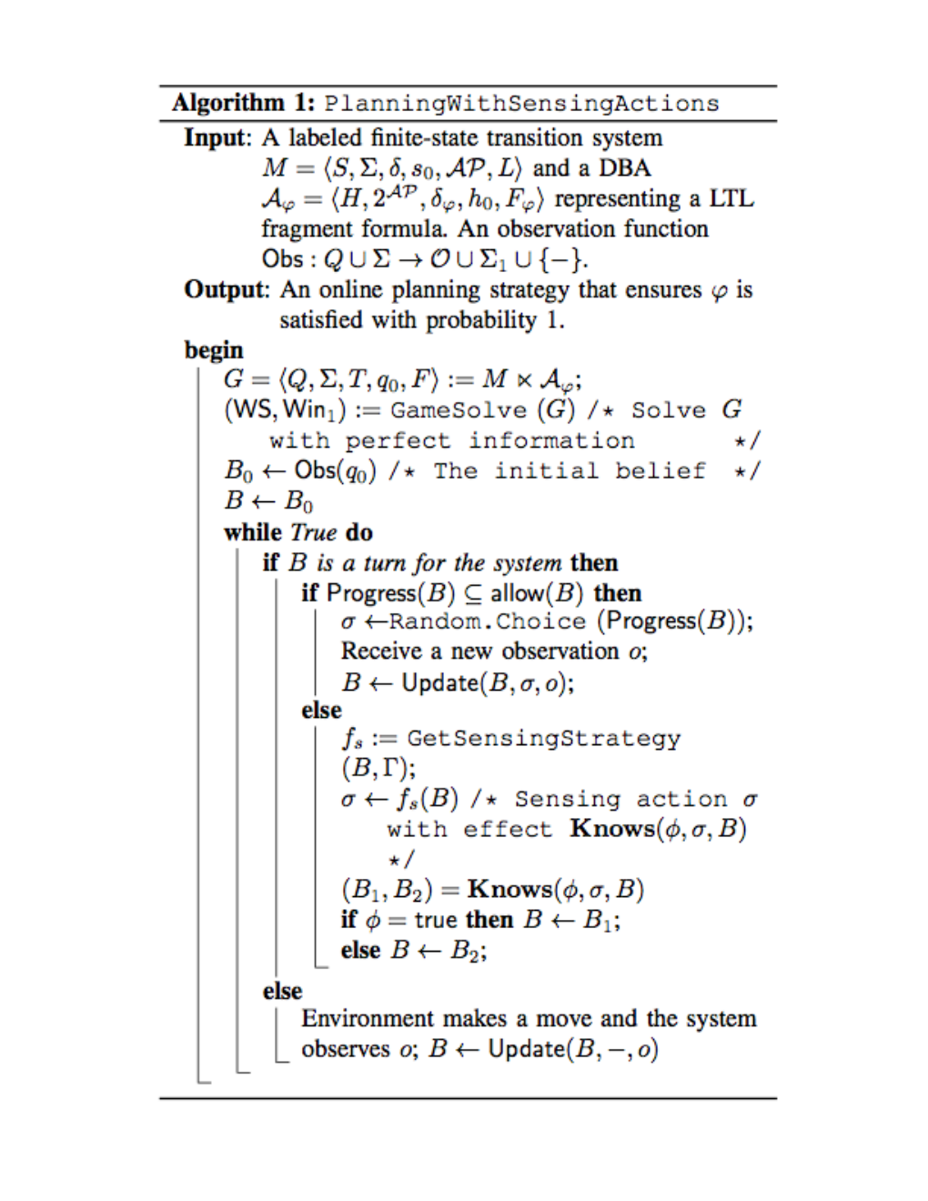
To conclude this section, Algorithm 1 describes the procedure of online planning with sensing actions.
IV Examples
We apply the algorithm to a robotic motion planning example, which is a variant of the so-called “Wumpus game” in a gridworld. Figure 2 consists of one mobile robot, one monster called “Wumpus”. The robot is capable of moving in eight compass directions with actions ‘N’, ‘S’ , ‘E’, ‘W’, ‘NE’, ‘NW’, ‘SE’, ‘SW’ (horizontally, vertically and diagonally), one step at a time. The robot and the Wumpus does not move concurrently. The Wumpus can move in four compass directions with actions ‘N’, ‘S’, ‘E’ and ‘W’ within a restricted area and emits stench to its surrounding cells. The objective of the robot is to infinitely revisit region , , and in this order, while avoiding running into the Wumpus. Formally, the temporal logic formula is where are the positions of the robot and the Wumpus, respectively. Yet, the robot only knows his own position. For this case of partial observation, without the inclusion of sensing actions, it can be shown that with the algorithms in [5], observation-based, sure-winning strategies and almost-sure winning strategies do not exist.

Here, we introduce a set of sensing actions to the game. For the robot to know the position of the moving obstacles, it needs to apply a sensing action — to detect if there exists stench at cell . Thus, when the robot applies , if the result is True, then the Wumpus must be some cells in the set . Otherwise, it is not possible that the Wumpus is in any cell in .
We illustrate how the robot updates his belief using sensing action where is a cell in the gridworld. Suppose that the robot does not know where the Wumpus is and hypothesizes it can be in any cell in the . Once it applies the sensing action , since the cell has stench and the sensor returns True. Then, immediately the robot will know the Wumpus is in one of the cells in the set , because only if the Wumpus is in a cell of , there can be stench in cell .
From the numerical experimental result, after steps (a step includes either a robot’s (sensing or physical) action or a movement of the Wumpus), the robot visited the set in the formulated two-player game times and can continue to visit infinite often. In Figure 3 we show the belief updates by applying alternatively the exploitation strategy and active sensing strategy for the initial steps. It is observed that the maximum cardinality of the belief set is over the control execution, which means that the robot thinks the Wumpus can be in any cell in its restricted region. However, if there is no danger of running into the Wumpus in a few next steps, there is no need to exercising any sensing action. The implementations are in Python on a desktop with Intel(R) Core(TM) i5 processor and 16 GB of memory. The average time for the robot making a decision is seconds. The computation of the product game took seconds and the winning strategy under complete information is computed within seconds.
V Conclusions
Our work shows that when additional information can be obtained through sensing actions, one can transform a sure-winning strategy with complete information to a belief-based, randomized strategy, which is then combined, at run time, with an active sensing strategy to ensure a given temporal logic specification is satisfied with probability 1. The synthesis method avoids a subset construction for solving games with partial information. Meanwhile, the active sensing strategy leads to a cost-efficient way of sensor design: Although we require a sufficient set of sensing actions to avoid dead-ends at run time, the system minimizes the usage of sensing actions by asking the most revealing queries, depending on what specification is to be satisfied, and how much uncertainty the system has about the game state at run time. In future work, we will consider more examples for practical robotic motion planning under partial observations. It is also important to consider the uncertainty in the sensors. For example, a sensor query might return a probabilistic distribution over a set of states, rather than a binary answer to proposition logical formulae considered herein. For this extension, we are currently investigating modifications that need to be made to account for delays, uncertainty in the information provided by the sensors.
References
- [1] Rajeev Alur and Salvatore La Torre. Deterministic generators and games for LTL fragments. ACM Transactions on Computational Logic, 5(1):1–25, January 2004.
- [2] A Arnold, A Vincent, and I Walukiewicz. Games for synthesis of controllers with partial observation. Theoretical Computer Science, 303(1):7–34, 2003.
- [3] Krishnendu Chatterjee and Laurent Doyen. The complexity of partial-observation parity games. In Logic for Programming, Artificial Intelligence, and Reasoning, pages 1–14. Springer, 2010.
- [4] Krishnendu Chatterjee and Laurent Doyen. Partial-Observation Stochastic Games: How to Win When Belief Fails. Annual IEEE Symposium on Logic in Computer Science, pages 175–184, June 2012.
- [5] Krishnendu Chatterjee, Laurent Doyen, Thomas A Henzinger, and Jean-François Raskin. Algorithms for omega-regular games with imperfect information. Logical Methods in Computer Science, 3(4):1–23, 2007.
- [6] Erich Grädel, Wolfgang Thomas, and Thomas Wilke, editors. Automata Logics, and Infinite Games: A Guide to Current Research. Springer-Verlag New York, Inc., New York, NY, USA, 2002.
- [7] M. Kloetzer and C. Belta. A fully automated framework for control of linear systems from temporal logic specifications. Automatic Control, IEEE Transactions on, 53(1):287–297, Feb 2008.
- [8] Hadas Kress-Gazit, Tichakorn Wongpiromsarn, and Ufuk Topcu. Correct, reactive robot control from abstraction and temporal logic specifications. IEEE Robotics and Automation Magazine, 18:65–74, 2011.
- [9] Michael Lederman Littman. Algorithms for sequential decision making. PhD thesis, Brown University, 1996.
- [10] Guy Shani and Ronen I Brafman. Replanning in domains with partial information and sensing actions. In IJCAI, volume 2011, pages 2021–2026, 2011.
- [11] Rangoli Sharan. Formal methods for control synthesis in partially observed environments : application to autonomous robotic manipulation. Dissertation (Ph.D.), California Institute of Technology. PhD thesis, California Institute of Technology, 2014.
- [12] Tichakorn Wongpiromsarn and Emilio Frazzoli. Control of probabilistic systems under dynamic, partially known environments with temporal logic specifications. In Proceedings of the 51th IEEE Conference on Decision and Control, CDC 2012, December 10-13, 2012, Maui, HI, USA, pages 7644–7651. IEEE, 2012.