Critical exponents for an impurity in a bosonic Josephson junction: position measurement as a phase transition
Abstract
We use fidelity susceptibility to calculate quantum critical scaling exponents for a system consisting of identical bosons interacting with a single impurity atom in a double well potential (bosonic Josephson junction). Above a critical value of the boson-impurity interaction energy there is a spontaneous breaking of symmetry corresponding to a second order quantum phase transition from a balanced to an imbalanced number of particles in either the left or right hand well. We show that the exponents match those in the Lipkin-Meshkov-Glick and Dicke models suggesting that the impurity model is in the same universality class. The phase transition can be interpreted as a measurement of the position of the impurity by the bosons.
pacs
03.75.Lm, 03.65.Ta, 67.85.Pq, 05.30.RtI Introduction
The fate of a single particle tunnelling in a many-body environment is a subject of fundamental interest not least because of its connection to the decoherence problem in quantum mechanics [1, 2]. In this paper we study a related system consisting of a single impurity atom tunnelling between the wells of a double well potential in the presence of indistinguishable bosonic atoms as illustrated schematically in Figure 1. The bosons are also trapped in the double well potential and thus form a bosonic Josephson junction in their own right. This setup can be considered to be an elementary example of a Bose-Fermi mixture although, because the statistics of the impurity do not matter, in practice it can be a boson of the same species but in a different internal state. The prospects for realizing such a system in the laboratory are reasonably promising: a large number of experiments have studied ultracold bosons trapped in external double well potentials [3, 4, 5, 6, 7, 8, 9, 10, 11], and others have realized the same effective system in a single trap but where two internal states of the atoms are coupled by microwave/radio frequency fields (internal Josephson effect) [12, 13]. Adding a well defined number of impurities is not easy but there has been some progress in this direction in optical lattices [14, 15].
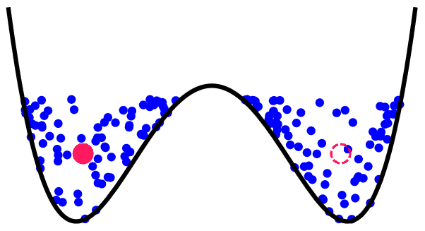
A theoretical analysis of a bosonic Josephson junction with an impurity has been given by Rinck and Bruder [16], who found that by applying a tilt to the double well a multi-particle tunnelling resonance could be induced towards a state where the impurity was expelled to the higher lying well. Subsequently, we undertook a study comparing the mean-field and many-body properties and described the appearance of a pitchfork bifurcation in the ground state of the mean-field theory above a certain critical value of the boson-impurity interaction strength [17]. The mean-field bifurcation arises from the spontaneous localization of the impurity in one of the wells together with a localization of a majority of bosons in the opposite well (assuming repulsive interactions). In the fully quantum version marks the onset of a splitting of the wave function into two coherent pieces in Fock space (the space spanned by the Fock states corresponding to the number differences and between the left and right wells for the impurity and bosons, respectively). As is increased further the Fock space splitting increases, and for large can develop into a fully blown Schrödinger cat state which is a superposition of two macroscopically distinguishable number differences of bosons. This state is associated with a saturation of the entanglement entropy between the impurity and the bosons at . The formation of a Schrödinger cat state in a macroscopic measurement device as a result of its coupling to a microscopic system is usually considered to be an essential element of quantum measurement [18, 19]. One may therefore take the view that the bosons in the present system act as a quantum measurement device or meter which indicates the position of the microscopic impurity atom. This meter can be tuned between being microscopic (small ) and macroscopic (large ). The formation and collapse of the Schrödinger cat state corresponds here to a symmetry breaking phase transition [20, 21, 22, 23, 24].
In another study [25], we argued that in many respects the impurity system behaves like the celebrated Dicke model [26, 27, 28] for two-level atoms coupled to a single mode of the electromagnetic field whose Hamiltonian takes the form
| (1) |
Here and annihilate and create, respectively, a photon of energy in the electromagnetic field and and are collective spin operators that arise from treating the two-level atoms, whose levels are separated by energy , as pseudospins. measures half the difference between the number of atoms in the excited state and the ground state and it eigenvalues lie in the range . measures the coherence between the excited and ground states of the atoms and is proportional to the position operator for the harmonic oscillator associated with the electromagnetic field. In a related pseudospin formulation the Hamiltonian for the bosonic Josephson junction plus impurity can be written (see Section II for details)
| (2) |
where the superscript ‘’ denotes the impurity: and are the bare hopping frequencies between the two wells for the bosons and impurity, respectively, and parameterizes the boson-impurity coupling strength. In this form the impurity model is reminiscent of the Mermin central-spin model where a distinguishable central-spin is surrounded by spins on a lattice which interact with the central spin with an effectively infinite range interaction so that all pairwise interactions have the same magnitude [29, 30, 31]. In the impurity model measures the coherence of the bosons between the two wells, or, equivalently, half the difference in the number of bosons in the antisymmetric and symmetric modes formed, respectively, from the odd and even combinations of the modes associated with each well. measures half the number difference between the two wells, or, equivalently, the coherence between their symmetric and antisymmetric combinations. and are the corresponding quantities for the impurity. In the thermodynamic limit where , the ground state of the Dicke model undergoes a second order phase transition due to a spontaneous breaking of symmetry at the critical coupling strength [32, 33]. This phase transition (PT) bears a very close resemblance to the bifurcation that occurs in the impurity model at [17, 25]
| (3) |
In the Dicke case the ground state below the transition () is known as the normal state and is characterized by and , whereas the ground state above the transition is known as the superradiant state because it corresponds to a spontaneous macroscopic excitation of the electromagnetic field with both and . Analogous ground states occur for the impurity model: when both the boson and the impurity probability distributions are symmetric and and both expectation values acquire finite values in the symmetry broken state occurring when . Furthermore, the dependence of the ground state energy upon the scaled parameters and is identical in the two models in the immediate vicinity of the transition [25]. It is also notable that the mean-field dynamics is in both cases regular below the transition and chaotic above it [27, 25]. In this paper we shall further investigate the bifurcation in the impurity model by calculating the critical exponents in order to establish whether it is indeed a second order phase transition in the same universality class as that in the Dicke model.
Although both the Dicke and Impurity models share many common features there is one glaring difference: the Dicke model couples spin-1/2 particles to a harmonic oscillator whereas the impurity model couples spin-1/2 particles to one other spin. In essence the impurity model truncates the harmonic oscillator Hilbert space to just two states, the ground state and the first excited state. The spin-1/2 representing the impurity can never become macroscopically excited like the simple harmonic oscillator can. It is therefore quite remarkable that the impurity model behaves like the Dicke model, but the critical exponents we calculate here show that very close to the transition a two-state Hilbert space for the harmonic oscillator in the Dicke model suffices to describe its critical properties.
In order to investigate the critical behavior and obtain the critical scaling exponents we shall calculate the fidelity susceptibility of the ground state. Over the past decade the concept of fidelity, which originated in quantum information theory [34], has gained wide use in analyzing critical behavior and classifying the universality of systems. It is most commonly used to quantify changes in the ground state of a system over a PT. This is done by calculating the product between the ground state with itself at different points in parameter space
| (4) |
where is the tunable parameter that drives the PT and is the ground state. It is expected that will tend to unity away from the critical region and reach a minimum when where the scalar product will be between the ground state below and above the critical point. One of the first phase transitions to be studied using the fidelity was the one-dimensional (1D) XY model where it was shown to decrease to a minimum near the critical point [35]. Furthermore, excited state fidelity has been used to characterize quantum phase transitions (QPT) where the ground state fidelity has failed [36]. Since the fidelity is a quantity depending only on the geometry of the Hilbert space and requires no knowledge of the order parameter it is useful in cases where the order parameter of a system is not obvious and has been studied in a variety of systems [37, 38, 39]. That being said, a more sensitive and natural quantity to study where no a priori knowledge of the system is needed, is the fidelity susceptibility (FS) [40, 41]. The FS measures the response of the fidelity to infinitesimal changes in the driving parameter of the system. It is closely related to the second derivative of the ground state energy with respect to the driving parameter, , so the FS is also similar to the magnetic susceptibility or specific heat when the driving parameters are the magnetic field and temperature, respectively. This means the FS can be used to study the critical behaviour of a system through calculations of scaling exponents.
In this paper we add to work done by others [42, 43, 44] regarding the scaling and criticality of bosons in a double well potential. We follow standard steps [45, 46] to show that the FS can be used to calculate scaling exponents for a general system. We then use the FS to focus on the critical behaviour of the two-site boson-impurity Hubbard model. The paper is organized in the following way: In Sec II we go into more detail about our model for the physical system under study. In Sec III we show how critical scaling exponents can be extracted from the FS. In Sec IV we apply the methods of Sec III to our system as well as extrapolate data to find numerical values for . In Sec V we find the FS critical exponents analytically and in Sec VI we give a summary and outlook for further work. Some of the details of the analytic calculations have been placed in an appendix.
II Model
We model the bosonic Josephson junction plus impurity system using the two-site Bose Hubbard Hamiltonian [16, 17]
| (5) |
Here, is the number difference operator between the two wells for the bosons and is the boson hopping operator. and are the equivalent operators for the impurity. The and subscripts denote the left and right modes and the creation/annihilation operators follow the usual bosonic commutation relations, i.e. with and all other combinations of the boson and impurity operators are zero. The scaling by in the first term in Eq. (5) is applied so that every term is and therefore takes a finite value in the thermodynamic limit. The pseudospin formulation of the Hamiltonian given in Eq. (2) is obtained from Eq. (5) by introducing the symmetric and antisymmetric combinations of the and modes: and , and then applying Schwinger’s oscillator model for angular momentum [47] and . An analogous set of transformations apply to the impurity.
We do not include direct boson-boson intra-well (or inter-well) interactions in our calculations and assume they can be removed (or the boson-impurity interaction enhanced) by a Feshbach resonance if necessary. We do this both to highlight the effect of the impurity and also because it turns out not to change the results in a qualitative way. Indeed, the nonlinearity due to the boson-boson interactions can lead to very similar results as those resulting from the boson-impurity interaction (the impurity can be viewed as mediating an effective interaction between the bosons). In the case of repulsive boson-boson interactions, a purely bosonic system has no PT in the ground state but does experience a symmetry breaking bifurcation in the excited states known as macroscopic self-trapping [48, 49] which has been seen in experiments [5]. If, on the other hand, the boson-boson interactions are attractive then there is a symmetry breaking PT in the ground state above a critical interaction strength where the bosons clump together in a single well. This PT has been studied by Buonsante et al [44] and we shall find that the PT in our system falls in the same universality class.
In previous work we found through stability analysis around the mean-field stationary points [25] that a pitchfork bifurcation of occurs at a critical value of the boson-impurity interaction given above in Eq. (3). For , and the bosons occupy each well equally. Above it becomes energetically favourable for the bosons to build-up in one well and the impurity to be localized in the opposite well. This transition corresponds to the breaking of the symmetry characterized by
| (6) |
We will consider as the driving parameter and will analyze the system’s response to infinitesimal changes in it through the FS.
III Fidelity susceptibility

As mentioned in the introduction, a more sensitive quantity than the fidelity is the FS which we shall denote by . The two are related through the Taylor expansion of Eq. (4) to second order
| (7) |
It can be viewed as the system’s response to an infinitesimal change in the driving parameter. Equation (5) has the general form
| (8) |
where is considered to be the driving term of the system. From perturbation theory [41] the FS is
| (9) |
where and are the th eigenstate and eigenenergy of the entire Hamiltonian, respectively. It is expected that for finite the FS scales as [45, 46]
| (10) |
where is the scaling exponent above and below the quantum critical point (QCP), respectively, is the value of at which is at a maximum, and is an intensive quantity. When will be limited by the size of the system, so we have
| (11) |
This quantity will diverge in the thermodynamic limit as . In fact, when Eq. (5) is divided by so that each term is rather than , then the exponent also gives the scaling of the energy gap between the ground and first excited states [50, 51] as we have verified [52]. Figure 2 illustrates how , which is given by the peak of each curve, depends on . In order to capture the behavior of both Eq. (10) and Eq. (11) we use the following form [45]
| (12) |
where is a constant and is a nonzero function of , both being intensive quantities. Since we are dealing with the susceptibility of the ground state wave function in the Fock basis, plays the role of the system size. With this in mind we can use the finite size scaling hypothesis [53] giving
| (13) |
where is the free energy density and is some function. We expect Eq. (13) to vanish as and at the same time the domain of the correlations to diverge. In this limit it is natural to expect [54]
| (14) |
where is the correlation length (in Fock space) and is the correlation length critical exponent. Combining Eqns. (13) and (14) gives the relation . Using the fact that in general the susceptibility due to is we can show the reduced FS is a universal function of and the driving parameter
| (15) |
where is some function. Finally, combining this equation with Eq. (12) gives us the important scaling relation
| (16) |
which we will use to help classify the boson-impurity system. It should be noted that Eq. (15) has been defined by others [46, 45] with the exponent of being instead of which we have here. In the next section we numerically evaluate the FS and guided by the above scaling hypotheses find the critical exponents by collapsing the data onto universal curves.

IV Numerical Results
Our results in this section are obtained by numerically diagonalizing the Hamiltonian given in Eq. (5). An boson system produces a matrix, so a system size of can be easily accommodated allowing us to obtain exact results. We note that due to symmetry parity is a conserved quantity, i.e. , and hence all the eigenvectors of our Hamiltonian are either even or odd in Fock space. Since we perform FS calculations on the ground state (which is of even parity) we can reduce the computation time by only considering even parity states. However, above the eigenstates typically come in even and odd pairs separated by an exponentially small energy difference and numerical diagonalization routines find it very hard to identify the parity of such eigenvectors. Unless one is careful numerical errors lead to eigenvectors with broken symmetry [17], and this directly impacts our results since it is the critical region we are concerned with in our calculations. We have outlined the resolution to this problem in the Appendix of our previous work [25] where we force the eigenstates to have definite parity by diagonalizing the Hamiltonian in the parity basis.
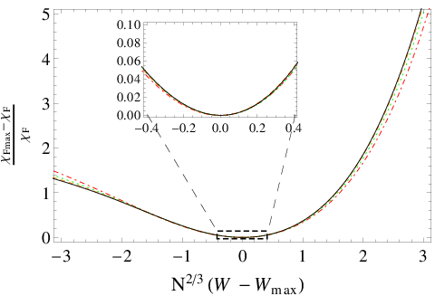
Figure 2 shows the results of plugging the numerically calculated eigenstates and energies for different system sizes into Eq. (9). We observe a clear peak in the FS for each value of which increases in height and sharpness as increases. This corresponds to the shrinking of the critical region and as . To find we first make a log-log plot of as a function of as shown in Fig. 3. We fit the curves to a second degree polynomial and extrapolate their slopes in the limit . From the inset we see that the slopes converge to a value of . We calculate for different values of to show that does not depend on and therefore is universal. Next, we use Eq. (15) to find by changing it in small increments until the average overlay of data points for different values of is maximized. Figure 4 shows the scaled in the vicinity of where a maximum overlay is achieved for . Figure 2 shows that below is an intensive quantity, so we have in Eq. (10). Above has a linear dependence on , so is an intensive quantity and . Using Eq. (16) to calculate we obtain and . These values of , and (keeping in mind the different definitions of ) are the same as those obtained for the Lipkin-Meshkov-Glick (LMG) model numerically [46] and analytically [55], for the Dicke model obtained numerically [56], as well as for the system consisting of bosons in a double well potential with attractive interactions obtained analytically [44]. This suggests that the boson-impurity system belongs in the same universality class as these models and that the QPT is second order.
We now shift our focus back to the convergence of to in the thermodynamic limit. Using the same steps used to determine we find the slope of a log-log plot of as a function of giving the convergence scaling exponent, , which we find to be the same as the inverse of the correlation length exponent, so . In Fig. 5 we show the effectiveness of the FS in predicting with extrapolation. For three different values of , using Eq. (3), we have compared to the extrapolated values of (all values are in units of ). With only five points of data we find the two sets of values to be in good agreement. Thus, if we were unable to find analytically, the FS would provide an excellent avenue to determine values numerically. We summarize our numerical results in Table 1 where the uncertainties are standard errors using a least-squares fit to our data.

| 0.25 (circle) | 0.75 (square) | 1.25 (triangle) | |
| 1.335(3) | 1.334(2) | 1.333(2) | |
| 1.499(2) | 1.504(5) | 1.502(3) | |
| 1 | |||
| 1.0062(2) | 1.7387(3) | 2.2432(3) |
V Analytic calculation of
In the thermodynamic limit the critical region collapses to a point and fluctuations vanish away from this point. For large systems away from the critical region this property allows us to use a mean-field approximation to analyze the FS. In previous work [17] we have shown that the mean-field Hamiltonian corresponding to Eq. (5) is
| (17) |
In we have defined and as the boson phase and number difference between the two wells, respectively, and and are similarly defined for the impurity. The conjugate nature of the number and phase variables means that Hamilton’s equations take the form
| (18) | |||
| (19) |
and the stable stationary solutions (which includes the ground state) of the system are
| (20) |
Note that for simplicity we have only displayed the solutions for the case when corresponding to a repulsive boson-impurity interaction. An intuitive understanding into the role of the impurity can be gained if we use the solutions in Eq. (20) to simplify Eq. (17) by adiabatically eliminating the impurity with the relation
| (21) |
giving us an effective Hamiltonian for the bosons alone
| (22) |
where . Setting for further simplification and scaling Eq. (22) by gives an effective Hamiltonian dependent on a single parameter, ,
| (23) |
A mean-field Hamiltonian of the same form occurs in the case of a purely bosonic Josephson junction where the microscopic origin of is direct boson-boson interactions [48, 49]. Specifically, the minus sign in front of the first term indicates effectively attractive boson-boson interactions. Although we have calculated here assuming repulsive boson-impurity interactions, it turns out to be unchanged for attractive interactions. Thus, the impurity always mediates attractive effective boson-boson interactions [57, 58], and it is for this reason that the PT in the impurity model falls into the same universality class as the clumping PT for attractive bosons. We can visualize how this happens by considering the impurity localized in one well and having , so the ground state will have a larger fraction of bosons in one well over the other. For the impurity expels bosons from the well it’s in and for bosons are attracted to the impurity. In both cases there is a build-up of bosons in one well over the other which is what happens when there are attractive boson-boson interactions.
An analytic calculation of the scaling exponents for the clumping transition for attractive bosons has been given in reference [44]. Their method for calculating the FS consists of approximating the ground state wave function as a Gaussian in Fock space centered at for and a symmetric superposition of Gaussians for . In our calculations we do not use a superposition of Gaussians for , but instead choose to have a single Gaussian centered at one of the two mean-field solutions, shown in Eq. (26), to represent the symmetry broken phase. The difference in these two approaches results in terms proportional to , so if we are sufficiently far from the critical region, then each approach is equivalent. Using a different form of the FS [61, 44]
| (24) |
they are able to calculate analytic expressions for the FS. Following their steps for Eq. (23), which we briefly outline in Appendix A, we obtain
| (25) |
We can see the scaling exponents are and agreeing with the numerical values calculated in the previous section. Equation (25) shows the leading order behaviour of the FS. Below there is a single leading term because the Gaussian wave function is fixed at , so changes in can only affect its size. Above changes in affect both the size and position of the wave function giving two terms where we see in the thermodynamic limit the position dependent term dominates.
VI Summary and Discussion
In this paper we have studied a symmetry breaking bifurcation in a bosonic Josephson junction driven by the interaction with an impurity atom. The fact that the maximum value of the FS, which can be viewed as a generalized susceptibility, diverges in the thermodynamic limit confirms that the symmetry breaking is associated with a second order phase transition (as expected from the continuous form of the bifurcation). By numerically calculating the critical scaling exponents of the FS and comparing them with those already known in the Dicke and LMG models, as well as for a system consisting of bosons in a double well potential with attractive interactions, we conclude that the PT in the impurity model lies in the same universality class as these other models. For the two exponents of the scaling of FS with on either side of the transition, we also carried out an analytic calculation and good agreement was found with the numerical result. We have also shown through extrapolation of in the thermodynamic limit that the FS can be used to predict numerically, and we find that it agrees with the analytic result calculated from the mean-field theory.
Interpreting the bosons as a meter measuring the position of the impurity, we have a particularly simple toy model for a binary quantum measurement in terms of a PT which occurs at a critical value of the system-meter interaction strength [20, 21, 22, 23, 24]. Quantum mechanically, the ground state probability distribution goes from having Gaussian fluctuations around to a superposition of two Gaussians each centered at one of the two bifurcating mean-field solutions. This latter state becomes a Schrödinger Cat state if and . Cat states are notoriously sensitive to perturbations and can be expected to rapidly collapse into one of the two wells thereby breaking the symmetry. This collapse is implicit in our model but it is interesting to ask whether a third agent beyond the impurity and the bosons is necessary to precipitate it. If the symmetry is broken by a classical field then it can be simply included in the Hamiltonian as a tilt to the double well potential [16, 17, 25] and as long as the perturbation is infinitesimal the PT is not affected. However, if the boson-impurity system is instead put into contact with a quantum mechanical environment then the effects can be more marked. PTs in open quantum systems (systems coupled to an environment) are now the subject of intensive research [62, 63], especially for the open Dicke model [64, 65, 66, 67]. One conclusion of this body of work is that the critical exponents can be modified by the coupling to the environment and this effect has been seen experimentally [68].
Finally, we mention that the impurity localization described in this paper is somewhat different to that found in the classic problem of an impurity in a uniform superfluid [69], or its modern descendant, an impurity in an extended gaseous Bose-Einstein condensate (BEC) [70, 71, 72, 73, 74]. For example, the Bose-Hubbard Hamiltonian employed here is a tight-binding model where the single particle wave functions (modes) are assumed to be unchanged by interactions, whereas the transition to a self-localized polaron state in an initially uniform BEC involves a change in the impurity wave function from delocalized to localized and the BEC develops a corresponding density dip. Furthermore, the type of symmetry that is broken in going from a uniform to a localized wave function is in general different to the binary choice underlying symmetry breaking (see Reference [75] for the case of a particle living on one and two-dimensional lattices with many lattice sites). However, in one dimensional extended systems the Josephson model underlying the physics studied here appears quite naturally as the impurity splits the BEC in two and we would expect there to be connections [76, 77]. We also point out that there are many other aspects to the impurity model and its close relatives beyond those discussed here, including how the coherence of the bosons is affected by the impurity [78, 17, 79], and system-bath dynamics [80, 81, 82, 83].
Acknowledgements.
We acknowledge insightful discussions with Jonas Larson and Sung-Sik Lee. This research was funded by the Natural Sciences and Engineering Research Council (NSERC) of Canada. JM also acknowledges funding from the government of Ontario.Appendix A Steps for Analytic Calculations
In this appendix we briefly outline the steps used to derive Eq. (25) from Eq. (23). We start by expanding Eq. (23) around the minima above and below
| (26) |
where . If we are sufficiently far away from , then is parabolic in shape around the minima, so the leading order term in the expansion will be the second giving a Schrödinger equation
| (27) |
where and
| (28) |
Equation (27) describes a harmonic oscillator in Fock space which means the ground state wave function will be a Gaussian of the form
| (29) |
The difference between the and wavefunctions is due to through Eq. (26) and the relation . With these forms of the ground state we can use Eq. (24) giving
| (30) |
and from here we obtain the expressions given in Eq. (25).
References
- [1] A. O. Caldeira and A. J. Leggett, Phys. Rev. Lett. 46, 211 (1981); Ann. Phys. (NY) 149, 374 (1983); 153, 445(E) (1984).
- [2] A. J. Leggett, S. Chakravarty, A. T. Dorsey, M. P. A. Fisher, A. Garg, and W. Zwerger, Rev. Mod. Phys. 59, 1 (1987).
- [3] Y. Shin, M. Saba, T. A. Pasquini, W. Ketterle, D. E. Pritchard, and A. E. Leanhardt, Phys. Rev. Lett. 92 050405 (2004); Y. Shin, C. Sanner, G.-B. Jo, T. A. Pasquini, M. Saba, W. Ketterle, D. E. Pritchard, M. Vengalattore and M. Prentiss, Phys. Rev. A 72, 021604(R) (2005); G.-B. Jo, J.-H. Choi, C. A. Christensen, T. A. Pasquini, Y.-R. Lee, W. Ketterle, and D. E. Pritchard, Phys. Rev. Lett. 98, 180401 (2007); G.-B. Jo, J.-H. Choi, C. A. Christensen, Y.-R. Lee, T. A. Pasquini, W. Ketterle, and D. E. Pritchard, Phys. Rev. Lett. 99, 240406 (2007).
- [4] Y.-J. Wang, D. Z. Anderson, V. M. Bright, E. A. Cornell, Q. Diot, T. Kishimoto, M. Prentiss, R. A. Saravanan, S. R. Segal, and S. Wu, Phys. Rev. Lett. 94, 090405 (2005).
- [5] M. Albiez, R. Gati, J. Fölling, S. Hunsmann, M. Cristiani, and M. K. Oberthaler, Phys. Rev. Lett. 95, 010402 (2005).
- [6] R. Gati, B. Hemmerling, J. Fölling, M. Albiez, and M. K. Oberthaler, Phys. Rev. Lett. 96, 130404 (2006); J. Estève, C. Gross, A. Weller, S. Giovanazzi, and M. K. Oberthaler, Nature (London) 455, 1216 (2008).
- [7] T. Schumm, S. Hofferberth, L. M. Andersson, S. Wildermuth, S. Groth, I. Bar-Joseph, J. Schmiedmayer and P. Krüger, Nature Phys. 1, 57 (2005); S. Hofferberth, I. Lesanovsky, B. Fischer, T. Schumm, and J. Schmiedmayer, Nature (London) 449, 324 (2007); T. Betz, S. Manz, R. Bücker, T. Berrada, Ch. Koller, G. Kazakov, I. E. Mazets, H.-P. Stimming, A. Perrin, T. Schumm, and J. Schmiedmayer, Phys. Rev. Lett. 106, 020407 (2011).
- [8] S. Levy, E. Lahoud, L. Shomroni and J. Steinhauer, Nature 449 579 (2007).
- [9] K. Maussang, G. E. Marti, T. Schneider, P. Treutlein, Y. Li, A. Sinatra, R. Long, J. Estève, and J. Reichel, Phys. Rev. Lett. 105, 080403 (2010).
- [10] F. Baumgärtner, R. J. Sewell, S. Eriksson, I. Llorente-Garcia, J. Dingjan, J. P. Cotter, and E. A. Hinds, Phys. Rev. Lett. 105, 243003 (2010).
- [11] L. J. LeBlanc, A. B. Bardon, J. McKeever, M. H. T. Extavour, D. Jervis, J. H. Thywissen, F. Piazza, and A. Smerzi, Phys. Rev. Lett. 106, 025302 (2011).
- [12] C. Gross, T. Zibold, E. Nicklas, J. Estève, and M. K. Oberthaler, Nature (London) 464, 1165 (2010); E. Nicklas, H. Strobel, T. Zibold, C. Gross, B. A. Malomed, P. G. Kevrekidis, and M. K. Oberthaler, Phys. Rev. Lett. 107, 193001 (2011).
- [13] T. Zibold, E. Nicklas, C. Gross, and M. K. Oberthaler, Phys. Rev. Lett. 105, 204101 (2010).
- [14] S. Will, T. Best, S. Braun, U. Schneider, and I. Bloch, Phys. Rev. Lett. 106, 115305 (2011).
- [15] R. Scelle, T. Rentrop, A. Trautmann, T. Schuster, and M. K. Oberthaler, Phys. Rev. Lett. 111, 070401 (2013).
- [16] M. Rinck and C. Bruder, Phys. Rev. A 83, 023608 (2011).
- [17] F. Mulansky, J. Mumford, and D. H. J. O’Dell, Phys. Rev. A 84, 063602 (2011).
- [18] J. von Neumann, Mathematische Grundlagen der Quantenmechanik (Springer, Berlin, 1932) [English translation by R. T. Beyer, Mathematical Foundations of Quantum Mechanics (Princeton University Press, Princeton, 1955)].
- [19] W. H. Zurek, Phys. Rev D. 26, 1862 (1982).
- [20] M. Damnjanovic, Phys. Lett. A 134, 77 (1988).
- [21] S. N. Mayburov in Quantum Communications and Measurement, V. P. Belavkin O. Hirota, and R. L. Hudson (Eds), (Springer Verlag, Berlin, 1995).
- [22] A. E. Allahverdyan, R. Balian, and T. M. Nieuwenhuizen, arXiv:quant-ph/0508162
- [23] N. Bar-Gill, G. Kurizki, B. A. Malomed, and C. Sudheesh, Phys. Rev. A 82, 013610 (2010).
- [24] P. A. Ivanov and D. Porras, Phys. Rev. A 88, 023803 (2013).
- [25] J. Mumford, J. Larson, and D. H. J. O’Dell, Phys. Rev. A 89, 023620 (2014).
- [26] R. H. Dicke, Phys. Rev. 93, 99 (1954).
- [27] C. Emary and T. Brandes, Phys. Rev. E 67, 066203 (2003).
- [28] B. M. Garraway, Phil. Trans. R. Soc. A 369, 1137 (2011).
- [29] H. P. Breuer, D. Burgarth, and F. Petruccione, Phys. Rev. B 70, 045323 (2004).
- [30] K. A. Al-Hassanieh, V. V. Dobrovitski, E. Dagotto, and B. N. Harmon, Phys. Rev. Lett. 97, 037204 (2006).
- [31] S. S. Garmon, P. Ribeiro, and R. Mosseri, Phys. Rev. E 83, 041128 (2011).
- [32] K. Hepp, E. H. Lieb, Ann. Phys. 76, 360 (1973).
- [33] Y. K. Wang and F. Hioe, Phys. Rev. A 7, 831 (1973).
- [34] M. A. Nielsen and I. L. Chuang, Quantum Computation and Quantum Information, (Cambridge University Press, Cambridge, UK, 2000).
- [35] P. Zanardi and N. Paunkovic, Phys. Rev. E 74, 031123 (2006).
- [36] S. Chen, L. Wang, S. J. Gu, and Y. Wang, Phys. Rev. E 76, 061108 (2007).
- [37] P. Buonsante and A. Vezzani, Phys. Rev. Lett. 98, 110601 (2007).
- [38] H. T. Quan, Z. Song, X. F. Liu, P. Zanardi, and C. P. Sun, Phys. Rev. Lett. 96, 140604 (2006).
- [39] W. Q. Ning, S. J. Gu, Y. G. Chen, C. Q. Wu, and H. Q. Lin, J. Phys. Condens. Matter 20, 235236 (2008).
- [40] W. L. You, Y. W. Li, and S. J. Gu, Phys. Rev. E 76, 022101 (2007).
- [41] M. F. Yang, Phys. Rev. B 76, 180403(R) (2007).
- [42] Z. Liu, H. Guo, S. Chen, and H. Feng, J. Phys. B: At. Mol. Opt. Phys. 45, 055301 (2012).
- [43] T. Sowinski, R. W. Chhajlany, O. Dutta, L. Tagliacozzo, and M. Lewenstein, arxiv:1304.4835 (2013).
- [44] P. Buonsante, R. Burioni, E. Vescovi, and A. Vezzani, Phys. Rev. A 85, 043625 (2012).
- [45] S. -J. Gu, H. -M. Kwok, W. -Q. Ning, and H. -Q. Lin, Phys. Rev. B 77, 245109 (2008).
- [46] H. -M. Kwok, W. -Q. Ning, S. -J. Gu, and H. -Q. Lin, Phys. Rev. E 78, 032103 (2008).
- [47] J. J. Sakurai, Modern Quantum Mechanics, (Addison-Wesley, New York, 1994).
- [48] G. J. Milburn, J. Corney, E. M. Wright, and D. F. Walls, Phys. Rev. A 55, 4318 (1997).
- [49] A. Smerzi, S. Fantoni, S. Giovanazzi, and S. R. Shenoy, Phys. Rev. Lett. 79, 4950 (1997).
- [50] N. T. Jacobson, S. Garnerone, S. Haas, and P Zanardi, Phys. Rev. B 79, 184427 (2009).
- [51] L. Campos Venuti and P. Zanardi, Phys. Rev. Lett. 99, 095701 (2007).
- [52] In other words, when is evaluated at using the eigenvalues of Eq. (5) as it stands it scales as as we have numerically verified.
- [53] V. Privman and M. E. Fisher, Phys. Rev. B 30, 322 (1984).
- [54] R. K. Pathria and R. D. Beale, Statistical Mechanics, (Elsevier, New York, 2011).
- [55] S. Dusuel and J. Vidal, Phys. Rev. Lett. 93, 237204 (2004); Phys. Rev. B 71, 224420 (2005).
- [56] T. Liu, Y. Y. Zhang, Q. H. Chen, and K. L. Wang, Phys. Rev. A 80, 023810 (2009).
- [57] H. Heiselberg, C. J. Pethick, H. Smith, and L. Viverit, Phys. Rev. Lett. 85, 2418 (2000).
- [58] D. H. Santamore and E. Timmermans, Phys. Rev. A 78, 013619 (2008).
- [59] L. Gong and P. Tong, Phys. Rev. B 78, 115114 (2008).
- [60] J. J. Jiang, Y. J. Liu, F. Tang, and C. H. Yang, Eur. Phys. J. B 83, 1-5 (2011).
- [61] M. Cozzini, R. Ionicioiu, and P. Zanardi, Phys. Rev. B 76, 104420 (2007).
- [62] S. Diehl, A. Micheli, A. Kantin, B. Kraus, H. P. Buechler, and P. Zoller, Nature Phys. 4, 878 (2008).
- [63] S. Gopalakrishnan, B. L. Lev, and P. M. Goldbart, Nat. Phys. 5, 845 (2009).
- [64] D. Nagy, G. Konya, G. Szirmai, and P. Domokos, Phys. Rev. Lett. 104, 130401 (2010); D. Nagy, G. Szirmai, and P. Domokos, Phys. Rev. A 84, 043637 (2011).
- [65] M. J. Bhaseen, J. Mayoh, B. D. Simons, and J. Keeling, Phys. Rev. A 85, 013817 (2012);
- [66] M. Öztop, M. Bordyuh, Ö. E. Müstecapliogu, and H. E. Türeci, New J. Phys. 14, 085011 (2012).
- [67] M. Buchhold, P. Strack, S. Sachdev, and S. Diehl, Phys. Rev. A 87, 063622 (2013).
- [68] F. Brennecke, R. Mottl, K. Baumann, R. Landig, T. Donner, and T. Esslinger, PNAS 110, 11763 (2013).
- [69] A. Miller, D. Pines and P. Nozieres, Phys. Rev. 127, 1452 (1962).
- [70] R. M. Kalas and D. Blume, Phys. Rev. A 73, 043608 (2006).
- [71] F. M. Cucchietti and E. Timmermans, Phys. Rev. Lett. 96, 210401 (2006).
- [72] J. Tempere, W. Casteels, M. K. Oberthaler, S. Knoop, E. Timmermans, and J.T. Devreese, Phys. Rev. B 80, 184504 (2009).
- [73] M. A. Cirone, G. De Chiara, G. M. Palma, and A. Recati, New J. Phys. 11, 103055 (2009).
- [74] E. Compagno, G. De Chiara, D. G. Angelakis, and G. M. Palma, arXiv:1410.8833 [quant-ph].
- [75] S. Dhar, S. Dasgupta, A. Dhar, and D. Sen, arXiv:1410.8701 [quant-ph].
- [76] M. Schecter, D. M. Gangardt, A. Kamenev, Annals of Physics 327, 639 (2012).
- [77] M. Schecter, A. Kamenev, D. M. Gangardt, and A. Lamacraft, Phys. Rev. Lett. 108, 207001 (2012).
- [78] I. Bausmerth, U. R. Fischer, and A. Posazhennikova, Phys. Rev. A 75, 053605 (2007); U. R. Fischer, C. Iniotakis, and A. Posazhennikova, ibid. 77, 031602(R) (2008).
- [79] P. Lu, Z.-H. Zhang, S. Feng, and S.-J. Yang, Phys. Rev. B 86, 104504 (2012).
- [80] D. Spehner and F. Haake, Phys. Rev. A 77, 052114 (2008).
- [81] G. Ferrini, D. Spehner, A. Minguzzi, and F. W. J. Hekking, Phys. Rev. A 82, 033621 (2010).
- [82] S. McEndoo, P. Haikka, G. De Chiara, G. M. Palma and S. Maniscalco, EPL 101, 60005 (2013).
- [83] S. Krönke, J. Knörzer, and P. Schmelcher, arXiv:1410.8676 [cond-mat.quant-gas].