Mixed finite elements for global tide models
Abstract
We study mixed finite element methods for the linearized rotating shallow water equations with linear drag and forcing terms. By means of a strong energy estimate for an equivalent second-order formulation for the linearized momentum, we prove long-time stability of the system without energy accumulation – the geotryptic state. A priori error estimates for the linearized momentum and free surface elevation are given in as well as for the time derivative and divergence of the linearized momentum. Numerical results confirm the theoretical results regarding both energy damping and convergence rates.
keywords
Finite element method, global tidal models, H(div) elements, energy estimates.AMS
65M12, 65M60, 35Q861 Introduction
Finite element methods are attractive for modelling the world’s oceans since implemention with triangular cells provides a means to accurately represent coastlines and topography [34]. In the last decade or so, there has been much discussion about the best choice of mixed finite element pairs to use as the horizontal discretization for atmosphere and ocean models. In particular, much attention has been paid to the properties of numerical dispersion relations obtained when discretizing the rotating shallow water equations [10, 6, 5, 21, 31, 23, 30, 22]. In this paper we take a different angle, and study the behavior of discretizations of forced-dissipative rotating shallow-water equations, which are used for predicting global barotropic tides. The main point of interest here is whether the discrete solutions approach the correct long-time solution in response to quasi-periodic forcing. In particular, we study the behavior of the linearized energy. Since this energy only controls the divergent part of the solution, as we shall see later, it is important to choose finite element spaces where there is a natural discrete Helmholtz decomposition, and where the Coriolis term projects the divergent and divergence-free components of vector fields correctly onto each other. Hence, we choose to concentrate on the mimetic, or compatible, finite element spaces (i.e. those which arise naturally from the finite element exterior calculus [1]) which were proposed for numerical weather prediction in [7]. In that paper, it was shown that the discrete equations have an exactly steady geostrophic state (a solution in which the Coriolis term balances the pressure gradient) corresponding to each of the divergence-free velocity fields in the finite element space; this approach was extended to develop finite element methods for the nonlinear rotating shallow-water equations on the sphere that can conserve energy, enstrophy and potential vorticity [29, 8, 26]. Here, we shall make use of the discrete Helmholtz decomposition in order to show that mixed finite element discretizations of the forced-dissipative linear rotating shallow-water equations have the correct long-time energy behavior. Since we are studying linear equations, these energy estimates then provide finite time error bounds.
Predicting past and present ocean tides is important because they have a strong impact on sediment transport and coastal flooding, and hence are of interest to geologists. Recently, tides have also received a lot of attention from global oceanographers since breaking internal tides provide a mechanism for vertical mixing of temperature and salinity that might sustain the global ocean circulation [27, 12]. A useful tool for predicting tides are the rotating shallow water equations, which provide a model of the barotropic (i.e., depth-averaged) dynamics of the ocean. When modelling global barotropic tides away from coastlines, the nonlinear advection terms are very weak compared to the drag force, and a standard approach is to solve the linear rotating shallow-water equations with a parameterised drag term to model the effects of bottom friction, as described in [20]. This approach can be used on a global scale to set the boundary conditions for a more complex regional scale model, as was done in [14], for example. Various additional dissipative terms have been proposed to account for other dissipative mechanisms in the barotropic tide, due to baroclinic tides, for example [16].
As mentioned above, finite element methods provide useful discretizations for tidal models since they can be used on unstructured grids which can seamless couple global tide structure with local coastal dynamics. A discontinuous Galerkin approach was developed in [32], whilst continuous finite element approaches have been used in many studies [18, 24, 11, for example]. The lowest order Raviart-Thomas element for velocity combined with for height was proposed for coastal tidal modeling in [33]; this pair fits into the framework that we discuss in this paper.
In this paper we will restrict attention to the linear bottom drag model as originally proposed in [20]. We are aware that the quadratic law is more realistic, but the linear law is more amenable to analysis and we believe that the correct energy behavior of numerical methods in this linear setting already rules out many methods which are unable to correctly represent the long-time solution which is in geotryptic balance (the extension to geostrophic balance of the three way balance between Coriolis, the pressure gradient and the dissipative term). In the presence of quasiperiodic time-varying tidal forcing, the equations have a time-varying attracting solution that all solutions converge to as . In view of this, we prove the following results which are useful to tidal modellers (at least, for the linear law):
- 1.
For the mixed finite element methods that we consider, the spatial semidiscretization also has an attracting solution in the presence of time-varying forcing.
- 2.
This attracting solution converges to time-varying attracting solution of the unapproximated equations.
Global problems require tidal simulation on manifolds rather than planar domains. For simplicity, our description and analysis will follow the latter case. However, our numerical results include the former case. Recently, Holst and Stern [15] have demonstrated that finite element analysis on discretized manifolds can be handled as a variational crime. We summarize these findings and include an appendix at the end demonstrating how to apply their techniques to our own case. This suggests that the extension to manifolds presents technicalities rather than difficulties to the analysis we provide here.
The rest of this paper is organised as follows. In Section 2 we describe the finite element modelling framework which we will analyse. In Section 3 we provide some mathematical preliminaries. In Section 4 we derive energy stability estimates for the finite element tidal equations. In Section 5 we use these energy estimates to obtain error bounds for our numerical solution. Appendix A includes the discussion of embedded manifolds.
2 Description of finite element tidal model
We start with the nondimensional linearized rotating shallow water model with linear drag and forcing on a (possibly curved) two dimensional surface , given by
| (1) |
where is the nondimensional two dimensional velocity field tangent to , is the nondimensional free surface elevation above the height at state of rest, is the (spatially varying) tidal forcing, is the Rossby number (which is small for global tides), is the spatially-dependent non-dimensional Coriolis parameter which is equal to the sine of the latitude (or which can be approximated by a linear or constant profile for local area models), is the Burger number (which is also small), is the (spatially varying) nondimensional drag coefficient and is the (spatially varying) nondimensional fluid depth at rest, and and are the intrinsic gradient and divergence operators on the surface , respectively.
We will work with a slightly generalized version of the forcing term, which will be necessary for our later error analysis. Instead of assuming forcing of the form , we assume some , giving our model as
| (2) |
It also becomes useful to work in terms of the linearized momentum rather than velocity. After making this substitution and dropping the tildes, we obtain
| (3) |
A natural weak formulation of this equations is to seek and so that
| (4) |
We now develop mixed discretizations with and . Conditions on the spaces are the commuting projection and divergence mapping onto . We define and as solutions of the discrete variational problem
| (5) |
We will eventually obtain stronger estimates by working with an equivalent second-order form. If we take the time derivative of the first equation in (5) and use the fact that , we have
| (6) |
where . This is a restriction of
| (7) |
which is the variational form of
| (8) |
to the mixed finite element spaces.
We have already discussed mixed finite elements’ application to tidal models in the geophysical literature, but this work also builds on existing literature for mixed discretization of the acoustic equations. The first such investigation is due to Geveci [13], where exact energy conservation and optimal error estimates are given for the semidiscrete first-order form of the model wave equation. Later analysis [9, 17] considers a second order in time wave equation with an auxillary flux at each time step. In [19], Kirby and Kieu return to the first-order formulation, giving additional estimates beyond [13] and also analyzing the symplectic Euler method for time discretization. From the standpoint of this literature, our model (3) appends additional terms for the Coriolis force and damping to the simple acoustic model. We restrict ourselves to semidiscrete analysis in this work, but pay careful attention the extra terms in our estimates, showing how study of an equivalent second-order equation in proves proper long-term behavior of the model.
3 Mathematical preliminaries
For the velocity space , we will work with standard mixed finite element spaces on triangular elements, such as Raviart-Thomas (RT), Brezzi-Douglas-Marini (BDM), and Brezzi-Douglas-Fortin-Marini (BDFM) [28, 4, 3]. We label the lowest-order Raviart-Thomas space with index , following the ordering used in the finite element exterior calculus [1]. Similarly, the lowest-order Brezzi-Douglas-Fortin-Marini and Brezzi-Douglas-Marini spaces correspond to as well. We will always take to consist of piecewise polynomials of degree , not constrained to be continuous between cells. In the case of domains with boundaries, we require the strong boundary condition on all boundaries.
In the main part of this paper we shall present results assuming that the domain is a subset of , i.e. flat geometry. In the Appendix, we describe how to extend these results to the case of embedded surfaces in .
Throughout, we shall let denote the standard norm. We will frequently work with weighted norms as well. For a positive-valued weight function , we define the weighted norm
| (9) |
If there exist positive constants and such that almost everywhere, then the weighted norm is equivalent to the standard norm by
| (10) |
A Cauchy-Schwarz inequality
| (11) |
holds for the weighted inner product, and we can also incorporate weights into Cauchy-Schwarz for the standard inner product by
| (12) |
We refer the reader to references such as [3] for full details about the particular definitions and properties of these spaces, but here recall several facts essential for our analysis. For all velocity spaces we consider, the divergence maps onto . Also, the spaces of interest all have a projection, that commutes with the projection into :
| (13) |
for all and any . We have the error estimate
| (14) |
when . Here, for the BDM spaces but for the RT or BDFM spaces. The projection also has an error estimate for the divergence
| (15) |
for all the spaces of interest, whilst the pressure projection has the error estimate
| (16) |
Here, and are positive constants independent of , , and , although not necessarily of the shapes of the elements in the mesh.
We will utilize a Helmholtz decomposition of under a weighted inner product. For a very general treatment of such decompositions, we refer the reader to [2]. For each , there exist unique vectors and such that , , and also . That is, is decomposed into the direct sum of solenoidal vectors, which we denote by
| (17) |
and its orthogonal complement under the inner product, which we denote by
| (18) |
Functions in satisfy a generalized Poincaré-Friedrichs inequality, that there exists some such that
| (19) |
We may also use norm equivalence to write this as
| (20) |
Because our mixed spaces are contained in , the same decompositions can be applied, and the Poincaré-Friedrichs inequality holds with a constant no larger than .
4 Energy estimates
In this section, we develop in stability estimates for our system, obtained by energy techniques. Supposing that there is no forcing or damping (), we pick and in (5), and find that
| (21) |
Since pointwise, we add these two equations together to find
| (22) |
Hence, we have the following.
Proposition 1.
In the absence of damping or forcing, the quantity
| (23) |
is conserved exactly for all time.
Now suppose that still but that pointwise in . The same considerations now lead to
| (24) |
so that
Proposition 2.
In the absence of forcing, but with , the quantity defined in (23) satisfies
In the presence of forcing and dissipation, it is also possible to make estimates showing worst-case linear accumulation of the energy over time.
Proposition 3.
With nonzero , we have that for all time ,
| (25) |
Proof.
We choose and as without forcing, and find that
Cauchy-Schwarz, Young’s inequality, and norm equivalence give
The result follows by dropping the positive term from the left-hand side and integrating. ∎
However, linear energy accumulation is not observed for actual tidal motion, so we expect a stronger result to hold. Turning to the second order equation (6), we begin with vanishing forcing and damping terms, putting to find
| (26) |
which simplifies to
| (27) |
so that the quantity
| (28) |
is conserved exactly for all time.
If is nonzero, we have that
| (29) |
which implies that is nonincreasing, although with no particular decay rate.
Now, we develop more refined technique based on the Helmholtz decomposition that gives a much stronger damping result. We can write in the -weighted decomposition. We let be a scalar to be determined later and let the test function in (6) be . This gives
| (30) |
and we rewrite the left-hand side so that
| (31) |
We use the fact that
and also that is -orthogonal to to rewrite the left-hand side as
| (32) |
This has the form of an ordinary differential equation
| (33) |
where
| (34) |
and
| (35) |
By showing that for suitably chosen , both and are comparable to defined in (28), we can obtain exponential damping of the energy.
Lemma 4.
Suppose that
| (36) |
Then
| (37) |
Proof.
Showing that is bounded above by a constant times is straightforward, but not needed for our damping results.
Lemma 5.
Suppose that
| (40) |
where
| (41) |
Then
| (42) |
Proof.
We use Cauchy Schwarz, the bounds and , and Young’s inequality with weight to write
| (43) |
Next, it remains to select and to make the coefficients of each norm positive and also balance the terms. First, we pick
and calculating that
we have that
| (44) |
We let be the solution to
so that
| (45) |
If we pick , then we have the lower bound for is exactly . However, we are also constrained to pick in order to guarantee that the lower bounds for is positive as well. If we have , then
and so we also have
| (46) |
∎
We combine these two propositions to give our exponential damping result.
Theorem 6.
Proof.
This result shows that the damping term drives an unforced system to one with a steady, solenoidal velocity field, in which the Coriolis force balances the pressure gradient term, i.e. in a state of geostrophic balance. Using the second equation in (5), we also know that the linearized height disturbance is steady in time in this case. These facts together lead to an elliptic equation for the steady state
| (50) |
It is easy to see that this problem is coercive on the divergence-free subspaces and thus is well-posed. Hence, with zero forcing, both and equal zero is the only solution. The zero-energy steady state then cannot have a nonzero solenoidal part. Moreover, the exponentially decay of toward zero forces to reach its steady state quickly, driving both and toward zero at an exponential rate. Finally, since almost everywhere, the exponential damping of also forces toward its zero steady state at the same rate.
Now, we turn to the case where the forcing term is nonzero, adapting this damping result to give long-time stability. The same techniques as before now lead to
| (51) |
Theorem 7.
For any and
| (52) |
we have the bound
| (53) |
Proof.
These stability results have important implications for tidal computations. Theorem 7 shows long-time stability of the system. Our stability result also shows that the semidiscrete method captures the three-way geotryptic balance between Coriolis, pressure gradients, and forcing. Moreover, we also can demonstrate that “spin-up”, the process by which in practice tide models are started from an arbitrary initial condition and run until they approach their long-term behavior, is justified for this method. To see this, the difference between any two solutions with equal forcing but differing initial conditions will satisfy the same (6) with nonzero initial conditions and zero forcing. Consequently, the difference must approach zero exponentially fast. This means that we can define a global attracting solution in the standard way (that is, take , for and as the solution starting from zero initial conditions at and define the global attracting solution as the limit as ), to which the solution for any condition becomes exponentially close in finite time. The error estimates we demonstrate in the next section then can be used to show that the semidiscrete finite element solution for given initial conditions approximates this global attracting solution arbitrarily well by picking large enough that the difference between the exact solution with those initial conditions and the global attracting solution is small and then letting be small enough that the finite element solution approximates that exact solution well.
5 Error estimates
Optimal a priori error estimates follow by applying our stability estimates to a discrete equation for the difference between the numerical solution and a projection of the true solution. We define
| (60) |
The projections and satisfy the first-order system
| (61) |
Subtracting the discrete equation (5) from this gives
| (62) |
By choosing the initial conditions for the discrete problem as and , the initial conditions for these error equations are
| (63) |
We start with estimates for the height and momentum variables, based on the stability result for the first order system.
Proposition 8.
For any , provided that ,
| (64) |
Proof.
Note that for any ,
Using this, that , and norm equivalence bounds the right-hand side above by
and the approximation estimate (14) finishes the proof. ∎
Since
we combine this result with the approximation estimates to obtain
Theorem 9.
If the above hypotheses hold, and also and , we have the error estimate
| (66) |
Note that our bound on the error equations in Proposition 8 depend only on the approximation properties of the velocity space, while the full error in the finite element solution depends on the approximation properties of both spaces. Consequently, the velocity approximation using BDM elements is suboptimal. Using RT or BDFM elements, both fields are approximated to optimal order.
Now, we use our estimates based on the second-order system to obtain error estimates for the time derivative and divergence of the momentum. The projection satisfies the perturbed equation
| (67) |
As in the first-order case, we have , and subtracting (6) from (67) gives
| (68) |
Theorem 7 and approximation estimates for give this result.
Proposition 10.
Let and suppose that . Then
| (69) |
Proof.
It is straightforward to get from here to a bound on the error
| (71) |
Theorem 11.
If the above assumptions hold, and also , then
| (72) |
6 Numerical results
In this section we present some numerical experiments that illustrate the estimates derived in the previous sections. In all cases the equations are discretized in time using the implicit midpoint rule. The domain is the unit sphere, centred on the origin, which is approximated using triangular elements arranged in an icosahedral mesh structure (see Appendix A for extensions of the results of this paper to embedded surfaces such as the sphere). All numerical results are obtained using the open source finite element library, Firedrake (http://www.firedrake.org).
First, we verify the energy behavior in the absence of dissipation, i.e. . The variables were initialized with and , and the equations were solved with parameters , , , and . The energy is conserved by the continuous-time spatial semi-discretization, and is quadratic. Since the implicit midpoint rule time-discretization preserves all quadratic invariants (see [25], for example), we expect exact energy conservation in this case; this was indeed observed as shown in Figure 1. Upon introducing a positive dissipation constant , we observe both that the energy is monotonically decreasing (as implied by Proposition 2), and is scaling exponentially in time (as implied by Theorem 6). These results are also illustrated in Figure 1.
Second, we verify the convergence results proved in Section 5. This was done by constructing a reference solution using the method of manufactured solutions, i.e. by choosing the solution
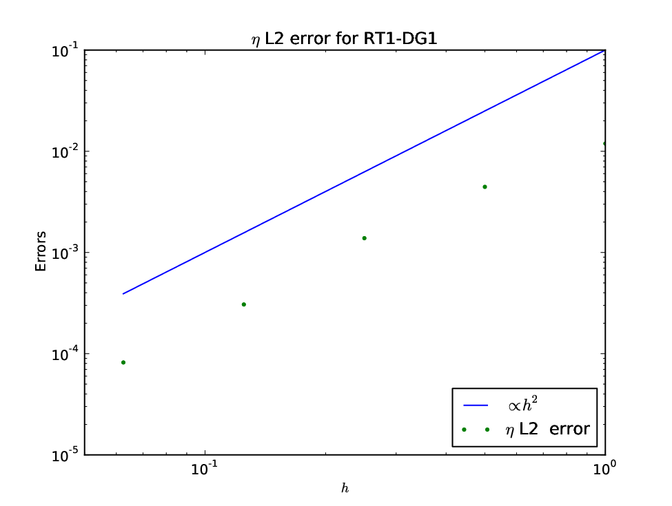
where we have expressed the velocity in three dimensional coordinates even though it is constrained to remain tangential to the sphere. Here and are chosen to solve the continuity equation for exactly, and is then chosen so that the equation is satisfied. We used the parameters , , , , and chose in order to isolate the error due to spatial discretization only. We ran the solutions until and computed the time-averaged error for . Plots are shown in Figure 2; they confirm the expected first order convergence rate for RT0, DG0, and the expected second order convergence rate for RT1, DG1.
Finally, we illustrate that this type of discretization excludes the possibility of spurious solutions. In the case of the linear forced-dissipative tidal equations with time-dependent forcing, the continuous equations have the property that the solutions lose memory of the initial conditions exponentially quickly with timescale determined from and the other parameters (and bounded by in Theorem 6). As discussed among our stability results, any two solutions with different initial conditions should converge to the same solution as . We illustrate this by randomly generating initial conditions for two solutions and with the same time-periodic forcing,
and measuring the difference between them as . In performing this test, care must be taken to ensure that and both have zero mean as implied by the perturbative derivation of the linear equations (since the dissipation cannot influence the mean component). In this experiment, we used the parameters , , and we used an icosahedral mesh of the sphere at the fourth level of refinement. We indeed observed that the two solutions converge to each other exponentially quickly in the norm, as illustrated in Figure 3.

7 Conclusions and future work
We have presented and analyzed mixed finite element methods for the linearized rotating shallow equations with forcing and linear drag terms. Our more delicate energy estimates rely on an equivalence between the first order form and a second order form, and this equivalence itself relies on fundamental properties of classical finite elements. In particular, our estimates show that the mixed spatial discretization accurately captures the long-term energy of the system, in which damping balances out forcing to prevent energy accumulation. Because of the linearity of the problem, our energy estimates also give rise to a priori error estimates that are optimal for Raviart-Thomas and Brezzi-Douglas-Fortin-Marini elements. Numerical results confirm both the stability and convergence theory given.
In the future, we hope to extend this work in several directions. First, we hope to study the more realistic quadratic damping model, which will require new techniques to handle the nonlinearity. Second, our estimates have only handled the semidiscrete case, and it is well-known that time-stepping schemes do not always preserve the right energy balances. Without damping or forcing, the implicit midpoint method preserves exact energy balance, and a symplectic Euler method will exactly conserve an approximate functional for linear problems. It remains to be seen how to give a rigorous fully discrete analysis, either including damping by a fractional step or fully implicit method. Finally, even explicit or symplectic time-stepping will require us to consider linear algebraic problems, as it is typically not possible to perform mass lumping for spaces on triangular meshes. Implicit methods will require additional care.
Appendix A Extension to the sphere and other embedded manifolds
Global tidal simulations are performed in spherical geometry, so it is necessary to consider mixed finite element discretization using meshes of isoparametric elements that approximate the sphere. This constitutes a variational crime since the domain supporting the mesh is only the same as the manifold in the limit . Recently, the topic of mixed finite elements on embedded manifolds was comprehensively analyzed by [15], following previous work on nodal finite elements. Here, we sketch out how to use their approach to extend the results of this paper to embedded manifolds.
In the case of curved domains such as the surface of the sphere, elements are implemented via Piola transforms from a reference triangle. This means that (a) the velocity fields are always tangential to the mesh element, and (b) normal fluxes take the same value on each side of element boundaries, as required to obtain a divergence that is bounded in (an approach to practical implementation of these finite element spaces on manifolds is provided by [29]). Similarly, the discontinuous spaces are implemented using a transformation from the reference triangle that includes scaling by the determinant of the Jacobian ; this ensures that the surface divergence maps from onto .
In this case , . [15] dealt with this problem by constructing operators and such that
where and are projections from to and to respectively; these two operators commute with defined on . In particular,
The estimates (14-16) then hold with and replacing and respectively, provided that the polynomial expansion of the element geometries in have at the same approximation order as and . There is also still a discrete Poincaré-Friedrichs inequality for . This means that all of our stability results 4 hold in the manifold case, and it remains to deal with the error estimates. This is done by introducing further variables , satisfying
| (73) |
This equation is of the form (5) but with a modified inner product on . Therefore, all of our stability estimates also hold for this modified equation.
We split the error in and by writing
| (74) |
where
| (75) |
We can bound and by applying Proposition 3 adapted to Equation (73), i.e. by substituting into (4) and rearranging so that it takes the form of (73) with a forcing defined in terms of , then subtracting (73). Similarly, and may be bounded by rearranging Equation (73) into the form of (4), then subtracting (4). Terms appear that are proportional to where
and is the maximum of the operator norms of and . [15] showed that converges to zero as with rate determined by the order of polynomial approximation in the isoparametric mapping. Hence we obtain a manifold version of Theorem 9, with and substituted by and respectively. Similar techniques lead to a manifold version of Theorem 11.
References
- [1] Douglas N. Arnold, Richard S. Falk, and Ragnar Winther, Finite element exterior calculus, homological techniques, and applications, Acta Numerica, 15 (2006), pp. 1–155.
- [2] , Finite element exterior calculus: from Hodge theory to numerical stability, Bulletin of the American Mathematical Society, 47 (2010), pp. 281–354.
- [3] Franco Brezzi and Michel Fortin, Mixed and hybrid finite element methods, Springer-Verlag New York, Inc., 1991.
- [4] Franco Brezzi, Jim Douglas Jr., and L. Donatella Marini, Two families of mixed finite elements for second order elliptic problems, Numerische Mathematik, 47 (1985), pp. 217–235.
- [5] R. Comblen, J. Lambrechts, J.-F. Remacle, and V. Legat, Practical evaluation of five partly discontinuous finite element pairs for the non-conservative shallow water equations, Int. J. Num. Meth. Fluid., 63 (2010), pp. 701–724.
- [6] C.J. Cotter and D.A. Ham, Numerical wave propagation for the triangular P1DG-P2 finite element pair, Journal of Computational Physics, 230 (2011), pp. 2806 – 2820.
- [7] CJ Cotter and J Shipton, Mixed finite elements for numerical weather prediction, Journal of Computational Physics, 231 (2012), pp. 7076–7091.
- [8] CJ Cotter and J Thuburn, A finite element exterior calculus framework for the rotating shallow-water equations, Journal of Computational Physics, 257 (2014), pp. 1506–1526.
- [9] Lawrence C. Cowsar, Todd F. Dupont, and Mary F. Wheeler, A priori estimates for mixed finite element methods for the wave equation, Computer Methods in Applied Mechanics and Engineering, 82 (1990), pp. 205–222.
- [10] S. Danilov, On utility of triangular C-grid type discretization for numerical modeling of large-scale ocean flows, Ocean Dynamics, 60 (2010), pp. 1361–1369.
- [11] M.G.G. Foreman, R.F. Henry, R.A. Walters, and V.A. Ballantyne, A finite element model for tides and resonance along the north coast of British Columbia, Journal of Geophysical Research: Oceans (1978–2012), 98 (1993), pp. 2509–2531.
- [12] Chris Garrett and Eric Kunze, Internal tide generation in the deep ocean, Annu. Rev. Fluid Mech., 39 (2007), pp. 57–87.
- [13] Tunc Geveci, On the application of mixed finite element methods to the wave equation, Math. Model. Numer. Anal, 22 (1988), pp. 243–250.
- [14] D.F. Hill, S.D. Griffiths, W.R. Peltier, B.P. Horton, and T.E. Törnqvist, High-resolution numerical modeling of tides in the western Atlantic, Gulf of Mexico, and Caribbean Sea during the Holocene, Journal of Geophysical Research: Oceans (1978–2012), 116 (2011).
- [15] Michael Holst and Ari Stern, Geometric variational crimes: Hilbert complexes, finite element exterior calculus, and problems on hypersurfaces, Foundations of Computational Mathematics, 12 (2012), pp. 263–293.
- [16] Steven R. Jayne and Louis C. St. Laurent, Parameterizing tidal dissipation over rough topography, Geophysical Research Letters, 28 (2001), pp. 811–814.
- [17] Eleanor W. Jenkins, Béatrice Rivière, and Mary F. Wheeler, A priori error estimates for mixed finite element approximations of the acoustic wave equation, SIAM Journal on Numerical Analysis, 40 (2002), pp. 1698–1715.
- [18] Mutsuto Kawahara and Kenichi Hasegawa, Periodic Galerkin finite element method of tidal flow, International Journal for Numerical Methods in Engineering, 12 (1978), pp. 115–127.
- [19] Robert C. Kirby and Thinh Tri Kieu, Symplectic-mixed finite element approximation of linear acoustic wave equations. submitted to Numerische Mathematik.
- [20] H. Lamb, ed., Hydrodynamics, Dover Publications, 6th ed., 1945.
- [21] D.Y. Le Roux, V. Rostand, and B. Pouliot, Analysis of numerically induced oscillations in 2D finite-element shallow-water models part I: Inertia-gravity waves, SIAM J. Sci. Comput., 29 (2007), pp. 331–360.
- [22] Daniel Y Le Roux, Spurious inertial oscillations in shallow-water models, Journal of Computational Physics, 231 (2012), pp. 7959–7987.
- [23] Daniel Y Le Roux and Benoit Pouliot, Analysis of numerically induced oscillations in two-dimensional finite-element shallow-water models part ii: Free planetary waves, SIAM journal on scientific computing, 30 (2009), pp. 1971–1991.
- [24] Fabien Lefevre, F.H. Lyard, Ch. Le Provost, and Erst J.O. Schrama, FES99: a global tide finite element solution assimilating tide gauge and altimetric information, Journal of Atmospheric and Oceanic Technology, 19 (2002), pp. 1345–1356.
- [25] Benedict Leimkuhler and Sebastian Reich, Simulating Hamiltonian dynamics, vol. 14, Cambridge University Press, 2004.
- [26] Andrew TT McRae and Colin J Cotter, Energy-and enstrophy-conserving schemes for the shallow-water equations, based on mimetic finite elements, Quarterly Journal of the Royal Meteorological Society, (2014).
- [27] Walter Munk and Carl Wunsch, Abyssal recipes II: energetics of tidal and wind mixing, Deep-Sea Research Part I, 45 (1998), pp. 1977–2010.
- [28] P. A. Raviart and J. M. Thomas, A mixed finite element method for 2nd order elliptic problems, in Mathematical aspects of finite element methods (Proc. Conf., Consiglio Naz. delle Ricerche (C.N.R.), Rome, 1975), Springer, Berlin, 1977, pp. 292–315. Lecture Notes in Math., Vol. 606.
- [29] Marie E. Rognes, David A. Ham, Colin J. Cotter, and Andrew T. T. McRae, Automating the solution of PDEs on the sphere and other manifolds in FEniCS 1.2, Geoscientific Model Development Discussions, 6 (2013), pp. 3557–3614.
- [30] V. Rostand and D.Y. Le Roux, Raviart-Thomas and Brezzi-Douglas-Marini finite-element approximations of the shallow-water equations, Int. J. Num. Meth. Fluids, 57 (2008), pp. 951–976.
- [31] Daniel Y. Le Roux, Dispersion relation analysis of the finite-element pair in shallow-water models, SIAM Journal on Scientific Computing, 27 (2005), pp. 394–414.
- [32] H. Salehipour, G.R. Stuhne, and W.R. Peltier, A higher order discontinuous Galerkin, global shallow water model: Global ocean tides and aquaplanet benchmarks, Ocean Modelling, 69 (2013), pp. 93–107.
- [33] Roy A Walters, Coastal ocean models: two useful finite element methods, Continental Shelf Research, 25 (2005), pp. 775–793.
- [34] Hilary Weller, Todd Ringler, Matthew Piggott, and Nigel Wood, Challenges facing adaptive mesh modeling of the atmosphere and ocean, Bulletin of the American Meteorological Society, 91 (2010), pp. 105–108.