Mixed semi-Lagrangian/finite difference methods for plasma simulations
Abstract.
In this paper, we present an efficient algorithm for the long time behavior of plasma simulations. We will focus on 4D drift-kinetic model, where the plasma’s motion occurs in the plane perpendicular to the magnetic field and can be governed by the 2D guiding-center model.
Hermite WENO reconstructions, already proposed in [25], are applied for solving the Vlasov equation. Here we consider an arbitrary computational domain with an appropriate numerical method for the treatment of boundary conditions.
Then we apply this algorithm for plasma turbulence simulations. We first solve the 2D guiding-center model in a D-shape domain and investigate the numerical stability of the steady state. Then, the 4D drift-kinetic model is studied with a mixed method, i.e. the semi-Lagrangian method in linear phase and finite difference method during the nonlinear phase. Numerical results show that the mixed method is efficient and accurate in linear phase and it is much stable during the nonlinear phase. Moreover, in practice it has better conservation properties.
Keywords. Cartesian mesh; semi-Lagrangian method; Hermite WENO reconstruction; guiding-center; drift-kinetic model.
2000 Mathematics Subject Classification. 65M08, 65M25, 78A35.
1. Introduction
In the context of strongly magnetized plasma simulations, the motion of particles is confined around the magnetic field lines; the frequency of this cyclotron motion is faster than the frequencies of interest. Therefore, the physical system can be reduced from the Vlasov-Maxwell system to a four or five dimensional model by averaging over the gyroradius of charged particles (See for a review [3, 14]). In this paper we focus on 4D drift-kinetic model, where the movement of the plasma in the plane perpendicular to the magnetic field can be governed by the guiding-center model. This reduced model could help us to investigate plasma turbulence problems with an acceptable computational time. More especially, using the 2D guiding-center model, we can focus directly on the difficulties of treatment of boundary conditions on arbitrary computational domain. Moreover, these reduced models have the conservative properties, which can be used as criterion to evaluate the good performance of numerical methods.
To develop accurate and stable numerical techniques for plasma turbulence (4D drift kinetic, 5D gyrokinetic and 6D kinetic models) is one of our objectives. In [15, 16] several numerical solvers have been developed using an Eulerian formulation for gyro-kinetic models. However, spurious oscillations often appear in the nonlinear phase when small structures occur and it is difficult to distinguish physical and numerical oscillations. Moreover, for these models semi-Lagrangian methods are no more conservative, hence the long time behavior of the numerical solution may become unsuitable. At contrast, a class of numerical methods based on the Hermite interpolation [10], together with a weighted essentially non-oscillatory (WENO) reconstruction can be applied either to semi-Lagrangian or to finite difference methods [25].
On the one hand, the semi-Lagrangian methods are very efficient and fast but do not conserve mass in an arbitrary grid. On the other hand, the finite difference methods are mass conservative and more stable for long term simulations but have a restrictive CFL constraint. We thus propose a mixed method to carry forward the advantages of each method, i.e. the semi-Lagrangian method in linear phase where the solution is relatively smooth, the finite difference method during the nonlinear phase where a lot of small structures appear. We will apply the mixed method to the 4D drift-kinetic model to verify its efficiency.
The numerical resolution of 4D drift-kinetic model in a cylinder has been already performed via polar coordinates [15]. However, polar coordinates are not always suitable since artificial singular points appear in the computational domain coming from the change of variable. Moreover, for more complicated geometry, it is not straightforward to perform the appropriate change of variables. From these considerations, we focus here on the discretization of transport models on a Cartesian mesh and develop a suitable technique as in [11] to treat boundary conditions. This method is based on the inverse Lax-Wendroff method [11]. On the other hand, to compute the electric potential from the Poisson equation, we apply an extrapolation technique [12]. To test the numerical algorithm, the guiding center model will be solved on a -shape domain [19]. We will first compute a steady state solution by solving numerically a nonlinear Poisson equation and then investigate its stability properties.
The paper is organized as follows : in Section 2, we present the derivation of the 4D drift-kinetic and the 2D guiding-center models, and their conservative properties. Then in Section 3, we recall the Hermite WENO reconstructions developed in [25] for solving the Vlasov equations, and the treatment of boundary conditions corresponding to the Poisson equation. In Section 4, we numerically compute a steady state solution for the 2D guiding-center model in a -shape domain. Then, we study its stability properties by performing numerical simulations with a perturbed steady state as initial data. Finally, we numerically solve the 4D drift-kinetic model with the mixed methods, and present the numerical results of the conservative properties of the 4D drift-kinetic model and the evolution of the distribution function of density.
2. Mathematical models
The Vlasov equation for the distribution function in standard form in standard notation is
| (2.1) |
where is the time variable, is the space variable, is the velocity variable, is the particle mass, is its charge, is the electric field and is the magnetic field. We assume the electric field is computed by , where is electric potential whereas the magnetic field is uniform , where stands for the unit vector in the toroidal direction. Moreover, we assume that is vanishing at infinity of velocity field and periodic boundary condition is taken in direction.
To derive the drift kinetic model, we start to perform a change of variable according to the drift direction ; that is
| (2.2) |
with
Next, we decompose into components along and perpendicular to :
Substituting this expression in (2.2), it yields
Then we introduce a new distribution function , such that
for which we get that it is solution to
Finally, we integrate the previous equation in velocity field
where . By passing formally to the limit , we obtain the drift-kinetic model
| (2.3) |
On the other hand, the self-consistent potential is solution to the quasi-neutrality equation [7]
| (2.4) |
where is the ion cyclotron frequency, and and are the electron temperature and density profiles respectively which only depend on . The ion density profile is given by
and represents the average on the magnetic field lines, that is,
with the length in the variable.
Dropping the over the various quantities and replacing by , the non-dimensional form of the drift-kinetic model can be written as
| (2.5) |
The following proposition shows some properties of the drift-kinetic model when we ignore the effect of boundary conditions:
Proposition 2.1.
Let us consider or the torus. Then the drift-kinetic model (2.5) verifies the following properties :
- (1)
If is smooth, we have the maximum principle
- (2)
norm conservation, for
- (3)
Kinetic entropy conservation
- (4)
Energy conservation
(2.6)
For practical applications, this model has to be supplemented with suitable boundary conditions when considering a domain of the form
with a two dimensional domain. We assume that the electric potential is vanishing at the boundary
| (2.7) |
and the distribution function is given by
| (2.8) |
where is a stationary solution to the drift-kinetic model (2.5). Furthermore, periodic boundary conditions are assumed for the potential and the distribution function in the direction
Finally, we can derive the guiding centre model from (2.5) by integrating the equation with respect to . We get that the reduced density is solution to the guiding centre system of equations
| (2.9) |
In this case, the solution satisfies the following properties
Proposition 2.2.
Let us consider the two dimensional domain or the torus. Then the guiding centre model (2.9) verifies the following properties :
- (1)
If is smooth, we have the maximum principle
- (2)
norm conservation, for
- (3)
Energy conservation
(2.10)
For practical applications, we assume that the electric potential is vanishing at the boundary
| (2.11) |
3. Numerical schemes
In this section we present the hybrid method based on the Hermite WENO reconstruction already proposed in [25]. On the one hand, we apply a semi-Lagrangian method for a general transport equation written in a non conservative form. On the other hand, we apply a finite difference method, which enforces the conservation of mass when the equation is written in the conservative form. These methods are coupled with the inverse Lax-Wendroff procedure to discretize accurately boundary conditions in an arbitrary geometry. Finally in the subsection 3.3, we discretize the Poisson equation for the electrical potential (2.9).
3.1. Hermite WENO reconstruction for semi-Lagrangian methods
We briefly remind the high order Hermite interpolation coupled with a weight essentially non-oscillatory (HWENO) reconstruction for semi-Lagrangian methods. The semi-Lagrangian method becomes a classical method for the numerical solution of the Vlasov equation because of its high accuracy and its small dissipation [5, 23]. For a given , the differential system
is associated to the transport equation
| (3.1) |
We denote its solution by . The backward semi-Lagrangian method is decomposed into two steps for computing the function at time from the function at time :
- (1)
For each mesh point of phase space, compute the backward characteristic , the value of the characteristic at time who is equal to at time .
- (2)
As the function of transport equation verifies
we obtain the value of by computing by interpolation, since is not usually a mesh point.
We apply a third order Hermite interpolation coupled with a weighted essentially non-oscillatory procedure, such that it is accurate for smooth solutions and it removes spurious oscillations around discontinuities or high frequencies which cannot be solved on a fixed mesh. Consider a uniform mesh of the computational domain and assume that the values of the distribution function and its derivative are known at the grid points. We define two quadratic polynomials in the interval :
The polynomial of degree 2 verifies
while verifies
The idea of WENO reconstruction is now to use the cubic polynomial when function is smooth, otherwise, we use the less oscillatory polynomial of degree 2 between or . Thus, let us define as follows
where and are WENO weights. To determine these WENO weights, we follow the strategy given in [18] and first define smoothness indicators by integration of the first and second derivatives of and on the interval :
Then we set and as
where
where , and to avoid the denominator to be zero.
Observe that when the function is smooth, the difference between and becomes small and the weights and . Otherwise, when the smoothness indicator , blows-up, then the parameter and the weight goes to zero, which yields
| (3.2) |
Finally, let us mention that the following fourth-order centred finite difference formula is used to approximate the first derivative at the grid point
| (3.3) |
3.2. Hermite WENO reconstruction for conservative finite difference methods
When the velocity is not constant in (3.1), the semi-Lagrangian method is not conservative even when , hence mass is no longer conserved and the long time behavior of the numerical solution may be wrong even for small time steps. Therefore, high order conservative methods may be more appropriate even if they are restricted by a CFL condition.
In this section, we extend Hermite WENO reconstruction for computing numerical flux of finite difference method. Suppose that is approximation of . We look for such that the flux difference approximates the derivative to -th order accuracy :
To approximate the flux , we define a piecewise polynomial such that it is exactly known on a set of points , .
Thus, given the point values , we can compute by an interpolation method and therefore deduce the numerical flux by
| (3.1) |
Now to interpolate the function , we apply a high order Hermite WENO scheme and outline the procedure of reconstruction only for the fifth order accuracy case.
The aim is to construct an approximation of the flux by the Hermite polynomial of degree five together with a WENO reconstruction from point values :
- (1)
We construct the Hermite polynomial such that
- (2)
We construct cubic reconstruction polynomials , , such that :
where is the sixth order centered approximation of first derivative
Let us denote by , , , the first derivatives of , , , respectively. By evaluating , , , at , we obtain
and
- (3)
We evaluate the smoothness indicators , , , which measure the smoothness of , , on the cell
- (4)
We compute the nonlinear weights based on the smoothness indicators
where the coefficients , , are chosen to get fifth order accuracy for smooth solutions and the parameter avoids the blow-up of , .
- (5)
The flux is then computed as
The reconstruction to is mirror symmetric with respect to of the above procedure.
3.3. Discretization of the Poisson equation (2.9)-(2.11)
We use a classical five points finite difference approximation to discretize the Poisson equation (2.9)-(2.11). So it remains to treat the Dirichlet boundary conditions on .
To discretize the Laplacian operator near the physical boundary, some points of the usual five points finite difference formula can be located outside of interior domain. For instance, Figure 1 illustrates the discretization stencil for at the point . We notice that the point is located outside of interior domain. Let us denote the approximation of at the point by . Thus should be extrapolated from the interior domain.
We extrapolate on the normal direction
| (3.2) |
where is the cross point of the normal and the physical boundary . The points and are equal spacing on the normal , i.e. , with , , are the space steps in the directions and respectively. Moreover, , , are the extrapolation weights depending on the position of , , and . In (3.2), is given by the boundary condition (2.11), whereas , should be determined by interpolation.
For this, we first construct an interpolation stencil , composed of grid points of . For instance, in Figure 1, the inward normal intersects the grid lines , , at points , , . Then we choose the three nearest points of the cross point , in each line, i.e. marked by a large circle. From these nine points, we can build a Lagrange polynomial . Therefore, we evaluate the polynomial at and , i.e.
with . We thus have that is approximated from the interior domain.
However, in some cases, we can not find a stencil of nine interior points. For instance, when the interior domain has small acute angle sharp, the normal can not have three cross points in interior domain, or we can not have three nearest points of the cross point , in each line. In this case, we alternatively use a first degree polynomial with a four points stencil or even a zero degree polynomial with an one point stencil. We can similarly construct the four points stencil or the one point stencil as above.
4. Numerical simulations
In this section, we present numerical simulations. We first consider the 2D guiding-center model in a D-shaped domain. The steady state solution and perturbed solution are studied. Then we perform the ion turbulence instability simulation with the 4D Drift-Kinetic model in a cylinder domain.
4.1. Test 1 : Steady state solution for the guiding center model in a D-shaped domain
We consider now the 2D guiding-center model in a D-shaped domain presented in Section IV of [19] and depicted in Figure 2(a). The mapping from curvilinear coordinates to physical coordinates is given by
for , .
 |
||
| (a) | (b) |
We now search a steady state solution for the guiding-center model in the D-shaped domain . We first notice that , a function of , is a solution of the guiding-center equation (2.9). Then it remains to solve a nonlinear elliptic equation
| (4.1) |
For a suitable function , we have a unique solution of equation (4.1) :
Proposition 4.3.
In the previous proposition, the existence of a positive solution is obtained by Schauder’s fixed point theorem [8], while the uniqueness is straight.
We now solve (4.1) in . Figure 2(b) illustrates that the boundary is embedded in Cartesian mesh. Thus the numerical scheme presented in section 3.3 should be applied, which gives us a nonlinear system for . Then by applying a Newton method to this nonlinear system, we obtain a steady state solution of (4.1) shown in Figure 3(a). Then by injecting into the guiding-center equation (2.9), we get the steady state density (see Figure 3(b)). Moreover, we plot the velocity field of steady state solution in Figure 4. By comparing the streamline in Figure 4 and the constant line of coordinates , it is interesting to notice that these lines don’t coincide, especially in the core of the D-shaped domain. The velocity is fast near the edge of the D-shaped domain but much slow in the core.
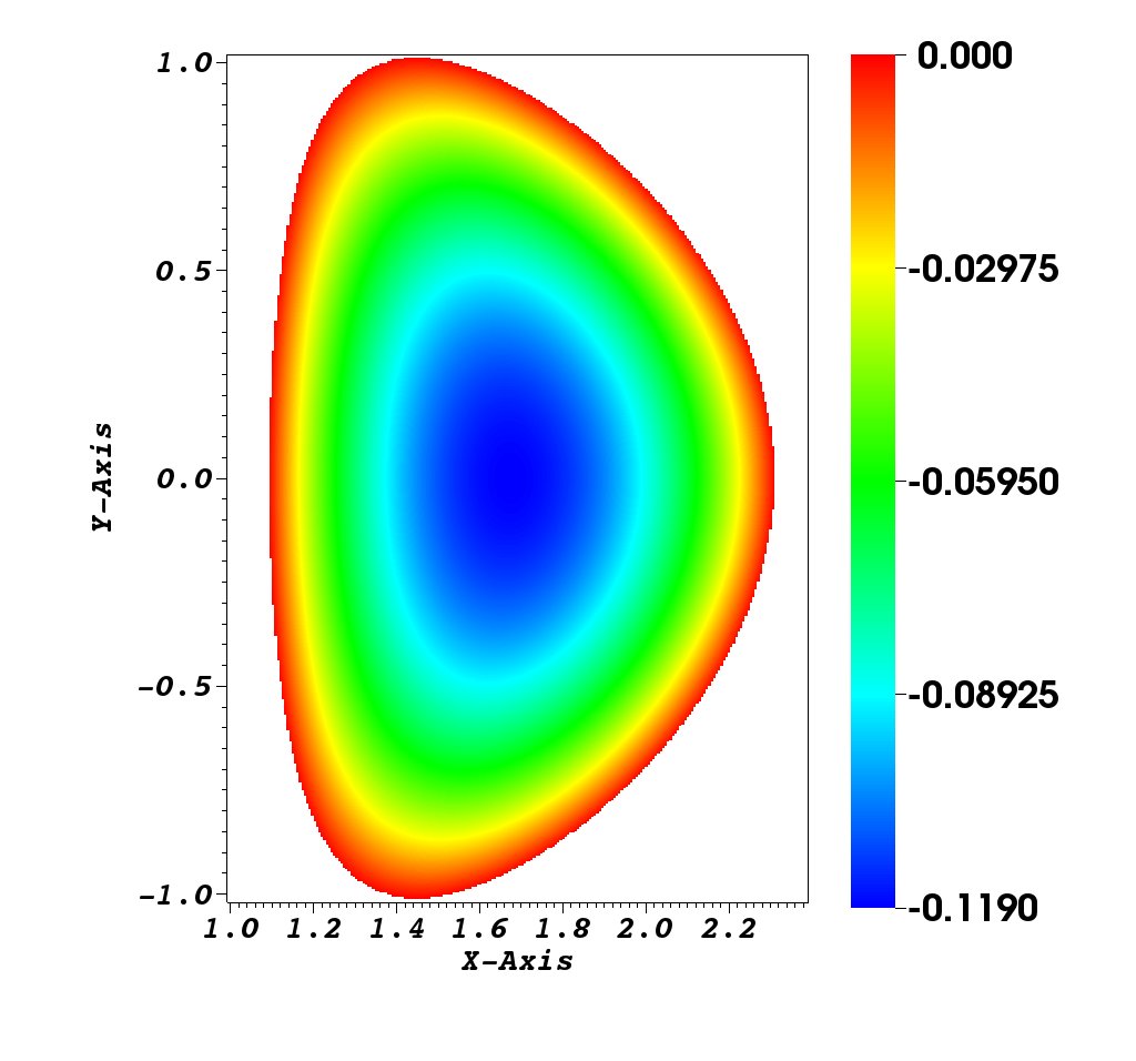 |
 |
| (a) Potential | (b) Density |
Now we verify that is the steady state solution by long time simulation. That is to take the pair as an initial solution for the guiding-center model (2.9), then to compare the difference between and . We will measure these differences by a relative error as
The finite difference method with HWENO reconstruction is used for solving guiding-center equation (2.9). The time step is taken to be . Figure 5 presents the relative errors of the potential and the density . We observe that the solution remains steady for long time simulation with a relative error of magnitude of .
| (a) Potential | (b) Density |
4.2. Test 2 : Numerical simulation of the guiding center model in a D shape
Now we still consider the previous initial data which is a stationary solution of the guiding-center model, but perturb it of magnitude of .
In Figure 4, we have noticed that the streamline is different with respect to the constant line of coordinates . On the other hand, we denote
Then by the definition of streamline, we have
which implies
Thus,
represents a streamline, i.e. the steady state function revolves along the isoline of potential . In this test case, we perturb the function along the streamline, that is
with , and .
Figure 6 illustrates the evolution of density governed by the guiding-center model. We present the difference between the perturbed density and the steady state density, i.e. . We observe that the difference of density revolves, and small filaments appear at time . Until the time , we can clearly identify the filaments.
 |
 |
| (a) | (b) |
 |
 |
| (c) | (d) |
4.3. Test 3 : Drift-kinetic model for ion turbulence simulation
In this subsection, we reproduce the ion turbulence simulation [15]. This simulation has been realized by different methods but in cylindrical coordinates [15, 21]. We will perform the simulation in Cartesian mesh with the numerical methods presented in section 3.
The discretization of the Drift-Kinetic model can be developed very similarly as the one for the guiding-center model. Here, we present some principle discretization steps.
The Vlasov equation of system (2.5) can be split into three equations :
Thus when applying the Semi-Lagrangian method, we use the Strang splitting method [22] for time discretization, and a second order predictor-corrector method for searching the characteristic foot. The Semi-Lagrangian method is suitable for linear phase simulation, because it doesn’t have CFL constraint and it is very accurate. However, it doesn’t preserve well the conservation properties of physical models [25] in nonlinear phase. Therefore, we should use the conservative finite difference method presented in section 3.2, where the 4th order Runge-Kutta method is used for time discretization. The criterion to pass from the Semi-Lagrangian to the finite difference methods is as follows
| (4.2) |
where is the smallest space step.
The quasi-neutrality equation of the system (2.5) is a three-dimensional elliptic problem. Obviously, a direct resolution of this equation is very costly. However, we notice that the diffusion term only depends on , and the second term of the quasi-neutrality equation is vanishing by taking average in -direction. Thus averaging the the quasi-neutrality equation in -direction, we get a 2D average equation
| (4.3) |
Taking difference between the quasi-neutrality equation and the average equation, it yields a fluctuation equation :
| (4.4) |
with . Note that the terms and are independent on . Thus the fluctuation equation (4.4) can be solve slice by slice in -direction. Moreover, the Dirichlet boundary conditions can also be decomposed for the average equation (4.3) and the fluctuation equation (4.4) as follows
Therefore, the resolution for Poisson equation in Section 3.3 can be applied for (4.3) and (4.4).
Now we perform the ion turbulence simulation. The plasma is initialized by exciting a single ion temperature gradient (ITG) model (where is a poloidal mode and is a toroidal mode). The distribution function is thus considered at the initial time as the sum of an equilibrium and a perturbed part: . The equilibrium part is chosen as a local Maxwellian
while the perturbation is determined as
where the profiles , and satisfy
together with the normalization
This gives the formulas
where and .
In this simulation, we choose the following parameters
Let us first compare the different discretization methods. The Semi-Lagrangian methods with cubic Hermite reconstruction and the HWENO reconstruction are used to solve the 4D Drift-Kinetic model, with small time step such that the CFL number is small than 1. Then we compare the numerical results with the one obtained by the mixed Semi-Lagrangian/finite difference method, where large time step (CFL) is used for the Semi-Lagrangian method in linear phase and small time step (CFL) is used in nonlinear phase. We emphasize that the Semi-Lagrangian method switches to the finite difference method automatically by the criterion (4.2).
In Figure 7, we summarize relative errors of the conservation laws for the Drift-Kinetic model for the different methods. We notice that these three methods have almost the same results when , while these results differ significantly when . We thus denote the linear phase for and the nonlinear phase for .
The Semi-Lagrangian methods can not conserve well the mass in the nonlinear phase, while the finite difference method conserve exactly the mass (see Figure 7(a)). Then from Figures 7(b), 7(c), we observe that the Semi-Lagrangian method with Hermite reconstruction loses completely the conservation properties for norm and entropy for long time simulation, since it involves too much spurious oscillation. At contrast, the Semi-Lagrangian method and the finite difference method with HWENO reconstruction work much better. Finally, we see the mixed Semi-Lagrangian/finite difference method has better energy conservation property than the Semi-Lagrangian methods in the nonlinear phase (see Figure 7(d)). Therefore, the mixed Semi-Lagrangian/finite difference method is better than the Semi-Lagrangian methods for long time ion turbulence simulation. Moreover, since the Semi-Lagrangian method is used in linear phase, thus our mixed method is more efficient than the pure finite difference method.
| (a) | (b) |
| (c) | (d) |
We next investigate the norm and entropy convergence properties of the mixed Semi-Lagrangian/finite difference method by refining mesh size in different directions. The results calculated with mesh size is used as a reference solution. In Figure 8, we observe that a significant improvement is obtained by refining in directions. The refinement in direction doesn’t improve the results. The ones obtained by refining in direction is slightly better than the reference solution. Figure 9 presents the refinement results for energy conservations. We see again the refinement in directions improves best the energy conservations.
| (a) | (b) |
| (c) | (d) |
| (e) | (f) |
| (a) | (b) |
| (c) | (d) |
At last, we present the evolution of the distribution function during ion turbulence simulation. We first notice in Figure 10 that the instability develops exponentially in the linear phase, where the growth of instability is measured by the quantity
where . Then the instability reaches a saturation point, which corresponds to the starting point of the nonlinear phase.
In Figure 11, we show the evolution of distribution function at . We see that till the time the instability can not be identified very clearly, that is why the Semi-Lagrangian method can be applied in the linear phase. At time , we reaches the saturation point, and five vortices are developed. These vortices rotate and create small filaments. At time , more small structures appear in the distribution function. At this moment, the Semi-Lagrangian method can not conserve well the invariant quantities, while the conservative finite difference method performs much better. Finally, the instability continues to develop small structures of the distribution function till the mesh size, and we attain to a relatively steady state.
 |
 |
| (a) | (b) |
 |
 |
| (c) | (d) |
 |
 |
| (e) | (f) |
5. Conclusion and perspective
In this paper, we have presented an efficient algorithm for long term plasma simulations. We first derive the 4D drift-kinetic and the 2D guiding-center models, and present their conservative properties. The Hermite WENO reconstructions are applied for solving the Vlasov equations, which was proved to be robust [25] in computational performance. Moreover, to adapt the arbitrary computational domain, we discretize the models on Cartesian meshes, and the special numerical methods for the boundary conditions, as the inverse Lax-Wendroff method for the Vlasov equation [11] and the extrapolation method for the poisson equation [12], are proposed.
Next, we solve the guiding-center model on a D-shape domain. A steady state solution is found numerically. Then we perturb the steady state density along the streamline, and use this perturbed density as the initial condition for the guiding-center model. We observe that the difference of density revolves, and the filaments appear for long term simulation.
Finally, we simulate the 4D drift-kinetic model with the mixed methods, i.e. the semi-Lagrangian method in linear phase and finite difference method during the nonlinear phase. Numerical results show that the mixed method is efficient and accurate in linear phase and it is much stable during the nonlinear phase. Moreover, it preserves well the conservative properties. We thus conclude that our mixed method is efficient for realistic and high dimensional plasma turbulence simulations.
Acknowledgment
Both authors are partially supported by the European Research Council ERC Starting Grant 2009, project 239983-NuSiKiMo and the Inria project Kaliffe. Chang YANG is also supported by National Natural Science Foundation of China (Grant No. 11401138).
References
- [1] F. Aràndiga, A. Baeza, A.M. Belda, and P. Mulet, Analysis of WENO Schemes for Full and Global accuracy, SIAM Journal on Numerical Analysis, 49(2) (2011), pp. 893-915.
- [2] A. Banon Navarro, P. Morel, M. Albrecht-Marc, D. Carati, F. Merz, T. Gorler and F. Jenko, Free energy cascade in gyrokinetic turbulence, Physical Review Letters, 106 (2011): 055001.
- [3] A. J. Brizard and T.S Hahm, Foundations of nonlinear gyrokinetic theory, Reviews of modern physics, 79 (2007), pp. 421–468.
- [4] C. Cercignani, The Boltzmann equation and its applications, Springer-Verlag, Berlin (1988).
- [5] C. Z. Cheng and G. Knorr, The integration of the Vlasov equation in configuration space, Journal of Computational Physics, 22 (1976), pp. 330–351.
- [6] P. Colella, M.R. Dorr, J.A.F. Hittinger and D.F. Martin, High-order, finite-volume methods in mapped coordinates, Journal of Computational Physics, 230 (2011), pp. 2952–2976.
- [7] N. Crouseilles, A. Ratnani, E. Sonnendrücker, An Isogeometric Analysis approach for the study of the gyrokinetic quasi-neutrality equation, Journal of Computational Physics, 231 (2012), 373–393.
- [8] L.C. Evans, Partial Differential Equations, Graduate Studies in Mathematics 19, AMS, 1998.
- [9] M.R. Feix, P. Bertrand, A. Ghizzo, Eulerian codes for the Vlasov equation, Series on Advances in Mathematics for Applied Sciences, Vol. 22, Kinetic Theory and Computing (1994), pp. 45–81.
- [10] F. Filbet, E. Sonnendrückder, Comparison of Eulerian Vlasov solvers, Compter Physics Communications, 150 (2003), 247–266.
- [11] F. Filbet and C. Yang, An inverse Lax-Wendroff method for boundary conditions of Boltzmann equations, Journal of Computional Physics, 245 (2013): 43–61.
- [12] F. Filbet and C. Yang, Numerical Simulations of Kinetic Models for Chemotaxis, SIAM Journal on Scientific Computing, 36(3) (2014) : B348–B366.
- [13] A. Ghizzo, P. Bertrand, M. Shoucri, T.W. Johnston, E. Filjakow, M.R. Feix, A Vlasov code for the numerical simulation of stimulated Raman scattering, Journal of Computional Physics, 90 (1990), pp. 431–457.
- [14] X. Garbet,Y. Idomura, L. Villard and T.H. Watanabe, Gyrokinetic simulations of turbulent transport, Nuclear Fusion, 50 (2010): 043002.
- [15] V. Grandgirard, M. Brunetti, P. Bertrand, N. Besse, X. Garbet, P. Ghendrih, G. Manfredi, Y. Sarazin, O. Sauter, E. Sonnendrücker, J. Vaclavik, L. Villard, A drift-kinetic Semi-Lagrangian 4D code for ion turbulence simulation, Journal of Computational Physics, 217 (2006), 395–423.
- [16] V. Grandgirard, Y. Sarazin, X. Garbet, G. Dif-Pradalier, Ph. Ghendrih, N. Crouseilles, G. Latu, E. Sonnendrücker, N. Besse, P. Bertran, Computing ITG turbulence with a full-f semi-Lagrangian code,Communications in Nonlinear Science and Numerical Simulation, 13 (2008), pp. 81–87.
- [17] A. Herten and S. Osher, Uniformly high-order accurate nonoscillatory schemes. I, SIAM Journal on Numerical Analysis, 24 (1987), pp. 279–309.
- [18] G.-S. Jiang and C.-W. Shu, Efficient implementation of weighted ENO schemes, Journal of computational physics, 126 (1996), pp. 202–228.
- [19] R.L. Miller, M.S. Chu, J.M. Greene, Y.R. Lin-Liu, R.E. Waltz, Noncircular, finite aspect ratio, local equilibrium model, Physical Plasmas, 5(4) (1998), pp. 973–978.
- [20] J. Pétri, Nonlinear evolution of the diocotron instability in a pulsar electrosphere: 2D PIC simulations, Astronomy & Astrophysics, 503 (2009), pp. 1–12.
- [21] R. Samtaney, Numerical aspects of drift kinetic turbulence: ill-posedness, regularization and a priori estimates of sub-grid-scale terms, Computational Science & Discovery, 5 (2012): 014004.
- [22] G. Strang, On the construction and comparison of difference schemes, SIAM Journal on Numerical Analysis, 5 (1968), pp. 506–517.
- [23] E. Sonnendrücker, J. Roche, The semi-Lagrangian method for the numerical resolution of Vlasov equation, Journal of computational physics, 149 (1999), pp. 201–220.
- [24] S. Tan and C.-W. Shu, Inverse Lax-Wendroff procedure for numerical boundary conditions of conservation laws, Journal of Computational Physics, 229 (2010), pp. 8144–8166.
- [25] C. Yang and F. Filbet, Conservative and non-conservative methods based on Hermite weighted essentially-non-oscillatory reconstruction for Vlasov equations, 279 (2014), pp. 18–36.