Backhaul-Constrained Multi-Cell Cooperation Leveraging Sparsity and Spectral Clustering

Rapid growth in wireless data traffic due to wide adoption of mobile devices has reinforced the research and development efforts to boost spectral efficiency of cellular networks. As the cell deployment becomes denser with a smaller cell size, it is recognized that inter-cell interference is a major bottleneck in provisioning desired link quality uniformly in the service area. Multi-cell cooperative processing (MCP), also referred to as network multi-input multi-output (MIMO), has shown promises for alleviating, and in many cases, exploiting, inter-cell interference. The idea is to have the base stations (BSs) collaborate in transmission and reception to/from the mobile stations (MSs), with the necessary coordination among the BSs taking place through the backhaul links [1]. The premise is that heavy interference experienced by the terminals residing at the cell boundaries is mitigated such that overall network throughput as well as fairness among users are improved. Field trials have verified that significant gain is indeed realizable [2, 3].

There are a number of approaches for implementing MCP [4, 3]. The BSs can loosely cooperate to avoid strong interference to/from the cell-edge users by exchanging channel state and scheduling information, and performing judicious power control and spatial filtering. When a high-speed low-latency backhaul network is available, more proactive and tighter coordination can be employed, where the antennas located at different BSs are transformed into a virtual antenna array. In the downlink, collaborating BSs can share transmitted symbols to engage in cooperative MIMO transmission. In the uplink, received signal samples at different BSs can be processed together to jointly decode multiple MSs. Such cooperative transmission and reception allow exploiting inter-cell interference constructively to actually improve link quality. Sophisticated coding strategies may also be adopted to expand the achievable rate region. As the dominant computational burden is still placed on the BSs, MSs can enjoy performance improvement at minimal increase in complexity.

To achieve the promised gain of MCP, important practical issues such as the finite backhaul capacity, latency, and synchronization issues must be addressed [5]. Unlimited backhaul capacity assumed in many of the earlier theoretical works is impractical for large cellular systems [6, 7]. Rather, the backhaul traffic volume must be contained in practice. In the same token, it may be infeasible to connect a large number of BSs to a central coordinator due to limitations in long-range backhauling. Instead, more localized communication structure may be desirable [8, 9]. Also, the channel state information may contain uncertainties due to practical training, quantization, and latency [10]. Maintaining synchronization across multiple cells is challenging. Moreover, complexity of various MCP algorithms may become prohibitive as the size of the network grows, calling for scalable distributed solutions.

The main focus of this work is to incorporate the limited backhaul rates. For instance, in the recent 3GPP (3rd Generation Partnership Project) Long Term Evolution (LTE) and LTE-Advanced cellular standards, the BSs can coordinate their trnasmission and reception by communicating over the logical X2 interface, or the S1 interface (through the core network), in the Coordinated Multi-Point (CoMP) transmission/reception mode [11]. The backhaul rate requirements vary depending on the specific methods of coordination. Coordinated scheduling of multiple BSs in the sub-frame timescale requires backhauling on the order of several hundred kbps [12]. For joint decoding, the requirement goes up to several Mbps [2, 3, 5]. Since analog signal samples (albeit in quantized or compressed formats) received from distributed antennas must be pooled together for joint processing, the backhaul overhead is quite significant in the uplink, compared to the downlink case where digital signals need to be shared [13]. Our focus in this work is on the most backhaul-intensive uplink joint decoding scenario.

Different models have been considered to capture the backhaul rate constraints [14]. A central coordination model assumes that all BSs are connected to a central station through finite-capacity backhaul links [15, 10]. The model is simple and thus amenable to theoretical analysis, but may have scalability and robustness issues in practical implementation. A distributed backhaul model assumes that the BSs can communicate with one another via finite-capacity backhaul links, which may be confined to a neighborhood [16, 17]. The backhaul capacity may be shared among the BSs for successive interference cancellation to achieve rates within a constant number of bits to the theoretical limits [18]. A third approach is to consider clusters of BSs that cooperate tightly, possibly with coordination across the clusters as well to a lesser degree [19, 20, 21].

Our approach is to design a linear combiner for joint decoding with the dual objectives of minimizing the mean-square error (MSE) of the combiner output, as well as the required backhaul rate. To perform joint decoding, a BS collects received signal samples at the neighboring BSs and combine them using a linear equalizer. The amount of the backhaul traffic¹¹ 1 In this work, the control signaling overhead is not explicitly captured in the backhaul overhead calculation, since it is negligible in comparison to the overhead due to sharing analog signal samples for joint decoding. The actual backhaul traffic rate, say in Mbps, depends on many implementation details such as the sampling frequency, quantization resolution, as well as various types of overhead. Therefore, in this work, what we term as the backhaul traffic captures the number of packets€ of samples transported from one BS to another BS through the backhaul network per unit time. Depending on how many samples (e.g. samples from multiple antennas at each BS) quantized with how many bits per sample are contained in one packet, the actual number in terms of Mbps will change. Also, due to this unspecified scaling, the backhaul traffic discussed in this work will not be represented in terms of particular units. incurred in this process is proportional to the number of the neighboring BSs from which the samples are collected. The number of cooperating BSs, in turn, is the same as the number of non-zero entries in the equalizer coefficient vector. To determine which coefficients to allow to be non-zero under the minimization objective requires a combinatorial search in principle. Our pragmatic approach is to adopt a convex relaxation of the problem in the spirit of the recent compressive sensing literature in order to design sparse equalizers [22].

Both distributed and clustered cooperation models are considered. In the distributed cooperation setup, each BS communicates directly with the cooperating BSs to obtain the signal samples. In the clustered scenarios, the BSs are partitioned into a number of non-overlapping clusters, and the signal samples are fully shared among the BSs in a cluster for joint decoding of the served MSs [20, 21]. It is assumed that the inter-cluster backhaul traffic constitutes the bottleneck, rather than the intra-cluster backhaul traffic. When the clusters are given and fixed, the equalizer weights corresponding to the inter-cluster feedback are sparsified. To solve jointly for dynamic clusters and equalizer weights, a spectral clustering approach is derived [23].

MCP in the downlink with limited backhaul rates has been investigated in the literature. Cooperative downlink transmission with per-BS power and Quality-of-Service (QoS) constraints was studied in [24]. A clustered cooperation scheme with linear processing in the downlink was proposed in [21]. In the context of multi-cell MIMO heterogeneous networks, joint BS clustering and beamformer design for downlink transmission were considered in [25, 26]. An energy-constrained beamformer design and BS-MS association for uplink and downlink were considered in [27]. Distributed precoder design and BS selection in a game theoretic framework were proposed in [28]. A semidefinite relaxation-based approach for backhual-limited cooperation in the downlink was proposed in [29]. Particle swarm optimization was used for zero-forcing-type beamformer design in [30]. Our work focuses on the uplink and does not require coordination with MSs, with all MCP burden placed on the BSs.

Direct exchanges of the signal samples between the BSs were considered in the context of 3GPP LTE systems in [13], where distributed cooperation without central control was advocated. Overlapping clusters of BSs were elected based on proximity for uplink MCP in [19]. A greedy algorithm for dynamic clustering was proposed to maximize the uplink sum-rate in [20]. Successive interference cancellation was adopted under limited backhaul traffic in [18], and cooperative group decoding was considered in a similar setting in [31]. Here, our intention is to concentrate on simple linear processing but address the backhaul traffic volume issue in both distributed and clustered cooperation settings in a consistent framework, and also derive distributed algorithms for scalable implementation.

Compared to our conference precursor [32], decentralized implementation of the proposed distributed and clustered cooperation schemes is developed in the present work. Decentralized computation of spatial equalizers and clusters makes MCP scalable to large networks, robust to isolated points of failure, and more resource-efficient than centralized implementation, since pieces of the overall problem are solved concurrently at different BSs, coordinated by peer message exchanges. Decentralized implementation of the component algorithms, such as group-sparse regression, eigenvector computation for network Laplacians, and k-means clustering, is also discussed. In addition, extensive simulations are performed to verify the performance, including the use of multiple antennas, user fairness, and dynamic clustered cooperation scenarios.

The rest of the paper is organized as follows. Sec. II introduces the system model. Sec. III develops backhaul-constrained distributed cooperation, while Sec. IV presents static and dynamic clustered cooperation. Decentralized implementation is the subject of Sec. V. Numerical tests are performed in Sec. VI, and conclusions are provided in Sec. VII.

Consider a multi-cell network uplink with $N_{B}$ BSs and $N_{U}$ MSs (users). Each BS $b\in{\mathcal{B}}:=\{1,2,\ldots,N_{B}\}$ is assumed to be equipped with $A$ antennas. Thus, the total number of BS antennas in the network is $N_{A}:=AN_{B}$. The set of antennas that belong to BS $b$ is denoted as ${\mathcal{A}}_{b}$. Each MS user $u\in{\mathcal{U}}:=\{1,2,\ldots,N_{U}\}$ possesses a single antenna. The serving BS of the $u$-th MS is denoted as $b(u)$. The set of MSs served by BS $b$ is denoted as ${\mathcal{U}}_{b}:=\{u\in{\mathcal{U}}:b(u)=b\}$.

Let $x_{u}$ denote the symbol transmitted by the $u$-th MS in a particular time slot and (sub-)band. Define ${\mathbf{x}}:=[x_{1},x_{2},$ $\ldots,x_{N_{U}}]^{T}$, where ^T stands for transposition. Similarly, the signal samples received by the $N_{A}$ BS antennas are represented as ${\mathbf{y}}:=[y_{1},y_{2},\ldots,y_{N_{A}}]^{T}$, where $y_{a}$ for $a\in{\mathcal{A}}:=\{1,2,\ldots,N_{A}\}$ denotes the sample taken by the $a$-th antenna. The flat-fading channel matrix ${\mathbf{H}}\in\mathbb{C}^{N_{A}\times N_{U}}$ has its $(a,u)$-entry equal to the complex channel coefficient from the $u$-th MS to the $a$-th BS antenna. Thus, the input-output relationship for the uplink can be expressed compactly as

$\displaystyle{\mathbf{y}}={\mathbf{H}}{\mathbf{x}}+{\mathbf{n}}$

(1)

where ${\mathbf{n}}$ represents additive noise and possible interference from outside the network. Vectors ${\mathbf{x}}$ and ${\mathbf{n}}$ are assumed to be zero-mean complex random vectors with covariance ${\mathbf{I}}$, which can be justified through prewhitening and normalization, as well as by absorbing MS transmit-powers into ${\mathbf{H}}$. It is also assumed that ${\mathbf{x}}$ and ${\mathbf{n}}$ are uncorrelated.

With MCP, multiple BSs cooperate to decode ${\mathbf{x}}$. For simplicity of implementation, linear receiver processing is considered. If all $N_{A}$ BS antennas in the network could fully cooperate, an estimate $\hat{\mathbf{x}}$ of ${\mathbf{x}}$ could be obtained using a linear equalizer ${\mathbf{W}}\in\mathbb{C}^{N_{U}\times N_{A}}$ as

$\displaystyle\hat{\mathbf{x}}={\mathbf{W}}{\mathbf{y}}$

(2)

where $\hat{\mathbf{x}}:=[\hat{x}_{1},\ldots,\hat{x}_{N_{U}}]^{T}$. Thus, in order to obtain the estimate $\hat{x}_{u}$ of $x_{u}$ of MS $u\in{\mathcal{U}}$, BS $b(u)$ would need to collect samples received by other BS antennas, and compute ${\mathbf{w}}_{u}^{T}{\mathbf{y}}$, where ${\mathbf{w}}_{u}^{T}$ denotes the $u$-th row of ${\mathbf{W}}$. A widely used linear equalizer, also adopted here, is the linear minimum mean-square error (LMMSE) one, given by

$\displaystyle{\mathbf{W}}_{\mathrm{lmmse}}$

$\displaystyle=({\mathbf{H}}^{\mathcal{H}}{\mathbf{H}}+{\mathbf{I}})^{-1}{\mathbf{H}}^{\mathcal{H}}$

(3)

where ^H denotes Hermitian transposition.

In the simplest cooperation model, henceforth termed distributed cooperation, each BS collects from cooperating BSs the received samples necessary for decoding its served MSs [13]. The set of cooperating BSs may overlap, in the sense that the set of BSs helping BS $b$ may have nonempty intersection with the set of BSs helping BS $b^{\prime}$ for $b\neq b^{\prime}$ [19, 33]. The BSs share the samples over the backhaul network. If unlimited backhaul traffic were allowed, every BS could collect samples from all other BSs to perform full cooperation. Since the backhaul capacity is limited in practice, each BS must judiciously choose the set of BSs whose samples are most helpful in decoding its intended MSs.

Given the equalizer matrix ${\mathbf{W}}$, the amount of backhaul traffic can be characterized. To get the basic idea, consider again the case of decoding MS $u$’s signal by forming ${\mathbf{w}}_{u}^{T}{\mathbf{y}}$. Clearly, collecting the entries in ${\mathbf{y}}$ that are measured by BSs other than the serving BS $b(u)$ must be conveyed to BS $b(u)$ through the backhaul links. These are the samples $\{y_{a}\}$ for $a\in{\mathcal{A}}\backslash{\mathcal{A}}_{b}$. However, if the $a$-th entry $w_{ua}$ of ${\mathbf{w}}_{u}^{T}$ is zero, then the corresponding entry $y_{a}$ need not be collected. Therefore, the actual backhaul traffic amount incurred is proportional to the number of nonzero entries in $\{w_{ua}\}_{a\in{\mathcal{A}}\backslash{\mathcal{A}}_{b(u)}}$.

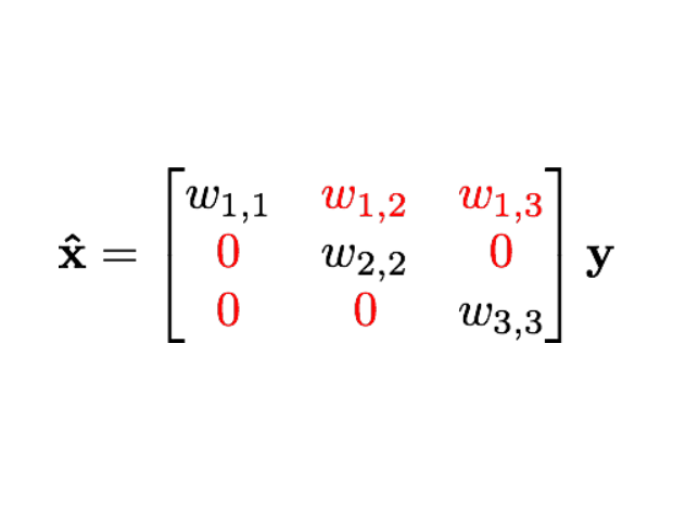
The idea can be applied straightforwardly in the case of single-antenna BSs; that is when $A=1$. Assume that $N_{B}=N_{U}=N_{A}$ with $b(u)=u$ for all $u\in{\mathcal{U}}$, and that the $b$-th antenna belongs to BS $b$; that is ${\mathcal{A}}_{b}=\{b\}$ for $b\in{\mathcal{B}}$. Then, under the distributed cooperation model, the amount of backhaul traffic is proportional to the number of nonzero off-diagonal entries of ${\mathbf{W}}\in\mathbb{C}^{N_{B}\times N_{B}}$. An illustration for the case with 3 BSs is provided in Fig. 1.

In the case of multi-antenna BSs with $A>1$, each BS may well serve more than one MS. There are two considerations to take into account when estimating the amount of backhaul traffic in the case of multi-antenna cell sites.

1. c1)

   Once BS $b$ has collected samples from a cooperating BS $b^{\prime}$ to decode a user $u\in{\mathcal{U}}_{b}$, no additional backhaul traffic is incurred even if these samples are used for decoding other MSs $u^{\prime}\neq u$ that are in ${\mathcal{U}}_{b}$. In other words, once the $(u,a^{\prime})$-entry of ${\mathbf{W}}$ is determined to be nonzero, where $u\in{\mathcal{U}}_{b}$ and $a^{\prime}\notin{\mathcal{A}}_{b}$, one can improve the decoding performance without incurring additional backhaul traffic by allowing $(u^{\prime},a^{\prime})$-entries of ${\mathbf{W}}$ to be nonzero for $u^{\prime}\in{\mathcal{U}}_{b}$.

2. c2)

   When a signal sample received from antenna $a\in{\mathcal{A}}_{b}$ is collected, it may be desirable to collect together the samples from all the antennas in ${\mathcal{A}}_{b}$ associated with that BS in order to economize the overhead due to backhaul packet headers and to maximize the MCP benefit.²² 2 As all-IP networking is advocated for cellular backhauling, the backhaul traffic is often routed using packet switching, which incurs header overhead. Assuming that the multiple antennas at a BS receive the MS signal at similar strengths, it is reasonable to collect all the samples from the multiple antennas together to maximize the MCP benefit. In this case, although the payload size increases linearly in the number of antennas, the header overhead is constant, as the samples may be aggregated into a single packet.

A way to succinctly capture c1) and c2) is to consider the set

$\displaystyle\left\{\sum_{u\in{\mathcal{U}}_{b}}\sum_{a\in{\mathcal{A}}_{b^{\prime}}}|w_{ua}|^{2}\Bigg|b,b^{\prime}\in{\mathcal{B}},\ b\neq b^{\prime}\right\}$

(4)

where it is worth noting that in order for an element to be zero, all squared terms in the sum must be zero. Thus, the backhaul traffic incurred is proportional to the number of nonzero elements in the set in (4).

In the clustered cooperation, BSs are partitioned into a number of non-overlapping clusters, and the received samples are fully shared among the BSs belonging to a cluster so that the MSs are served jointly [20, 21]. Since the clusters do not overlap, the cluster-edge users may suffer from interference [34]. In some cases, natural clustering could emerge by the deployment constraints of the network, such as the hierarchical routing architecture of the backbone network, or the geographical proximity of the cell sites. In other cases, dynamic formation and adaptation of clusters may be beneficial. In the latter case, clusters themselves can be optimized based on channel gains or traffic patterns [20].

It is assumed that inter-cluster backhaul traffic is more costly to the backhaul network than intra-cluster traffic. For example, when multiple cells are controlled by a single cell tower, backhauling between these cell sites are virtually free. Similarly, the particular routing topology of the backhaul implementation may dictate certain backhauling paths are much cheaper than others. Inter-cluster backhaul traffic may pass through multiple layers of routing hierarchy, incurring higher signaling overhead. The precise mathematical backhaul traffic characterization will be presented in Sec. IV. Next, the two modes of MCP operation will be studied one by one.

For simplicity of exposition, consider first the case with $A=1$, $N_{B}=N_{U}=N_{A}$, ${\mathcal{U}}_{b}=\{b\}$ and ${\mathcal{A}}_{b}=\{b\}$ for all $b\in{\mathcal{B}}$, as in Sec. II-B. Since the amount of backhaul traffic is proportional to the number of nonzero off-diagonal entries of ${\mathbf{W}}$, a natural approach to obtain a backhaul-constrained MCP solution is to promote sparsity in the off-diagonal entries of ${\mathbf{W}}$ (that is, favor many zero entries in the off-diagonal positions with minimal sacrifice in the MCP gain). Inspired by recent advances in compressive sensing techniques, the idea here is to optimize the cost functions related to the MMSE criterion, augmented with sparsity-promoting regularization terms [22, 35].

Let $\tilde{\mathbf{W}}\in\mathbb{R}^{N_{B}\times N_{B}}$ denote the matrix with zero diagonal entries, and the off-diagonal entries equal to the absolute values of the corresponding entries in ${\mathbf{W}}$.³³ 3 Since the entries of ${\mathbf{W}}$ are complex numbers, setting an entry to zero amounts to setting both the real and the imaginary parts of the entry to zero. Considering the absolute value of the complex entry satisfies this requirement, and leads later to the group sparsity formulation quite naturally [36]. More discussion on group sparsity will be provided in Sec. III-B. The LMMSE equalizer seeks to minimize the mean-square error (MSE) ${\mathbb{E}}\{||\hat{\mathbf{x}}-{\mathbf{x}}||_{2}^{2}\}=||{\mathbf{I}}-{\mathbf{W}}{\mathbf{H}}||_{F}^{2}+||{\mathbf{W}}||_{F}^{2}$. Thus, one can penalize large values of $\ell_{0}$-“norm” of $\tilde{\mathbf{W}}$ as in

$\displaystyle\min_{{\mathbf{W}}}\|{\mathbf{I}}-{\mathbf{W}}{\mathbf{H}}\|_{F}^{2}+\|{\mathbf{W}}\|_{F}^{2}+\lambda\|\tilde{\mathbf{W}}\|_{0}$

(5)

where $\|\tilde{\mathbf{W}}\|_{0}$ denotes the total number of nonzero entries in $\tilde{\mathbf{W}}$, $\|\cdot\|_{F}$ the Frobenius norm, and $\lambda$ controls the amount of backhaul traffic incurred by the solution.

Since the criterion in (5) is nonconvex, to obtain a solution efficiently, we advocate replacing the $\ell_{0}$-“norm” with the $\ell_{1}$-norm, which offers the tightest convex relaxation of the $\ell_{0}$ counterpart. Thus, the relevant optimization problem is

$\displaystyle\min_{{\mathbf{W}}}||{\mathbf{I}}-{\mathbf{W}}{\mathbf{H}}||_{F}^{2}+||{\mathbf{W}}||_{F}^{2}+\lambda||\tilde{\mathbf{W}}||_{1}$

(6)

which is equivalent to

$\displaystyle\min_{{\mathbf{W}}}\left\|\bar{\mathbf{I}}-{\mathbf{W}}\bar{\mathbf{H}}\right\|_{F}^{2}+\lambda||\tilde{\mathbf{W}}||_{1}$

(7)

where $\bar{\mathbf{I}}:=\big[{\mathbf{I}}\ \ \mathbf{0}\big]$, $\bar{\mathbf{H}}:=\big[{\mathbf{H}}\ \ {\mathbf{I}}\big]$, and $\|\tilde{\mathbf{W}}\|_{1}$ is the sum of the (absolute) values of all entries of $\tilde{\mathbf{W}}$.

Considerations c1) and c2) discussed in Sec. II-B for characterizing the backhaul traffic naturally impose certain structural constraints in sparsifying ${\mathbf{W}}$ in the multi-antenna case. That is, for any pair of BSs $b$ and $b^{\prime}$ with $b\neq b^{\prime}$, the weights $w_{ua}$ for $u\in{\mathcal{U}}_{b}$ and $a\in{\mathcal{A}}_{b^{\prime}}$ should be constrained to be either all zero or all nonzero.

Such a structure can be effected using penalty terms promoting group sparsity [36]. When a vector ${\mathbf{w}}\in\mathbb{R}^{N}$ is partitioned to $J$ subvectors as ${\mathbf{w}}:=[{\mathbf{w}}_{1}^{T},{\mathbf{w}}_{2}^{T},\ldots,{\mathbf{w}}_{J}^{T}]^{T}$ with ${\mathbf{w}}_{j}\in\mathbb{R}^{N_{j}}$ and $\sum_{j=1}^{J}N_{j}=N$, rather than pursuing the sparsity of the individual entries in ${\mathbf{w}}$ independently by using a penalty term of the form $\lambda\|{\mathbf{w}}\|_{1}$, one can encode group structures by using $\lambda\sum_{j=1}^{J}\|{\mathbf{w}}_{j}\|_{2}$. This gives rise to ${\mathbf{w}}_{j}$’s that are either entirely zero or nonzero.

Under these considerations, one can replace the penalty term in (7) with

$\displaystyle\lambda\sum_{b,b^{\prime}\in{\mathcal{B}}:b\neq b^{\prime}}\sqrt{\sum_{u\in{\mathcal{U}}_{b}}\sum_{a\in{\mathcal{A}}_{b^{\prime}}}|w_{ua}|^{2}}$

(9)

where $w_{ua}$ is the $(u,a)$-entry of ${\mathbf{W}}$. The first sum inside the square root collects the entries for all served MSs in BS $b$, and the second one for all the antennas in a cooperating BS $b^{\prime}$. Another way of expressing this is by defining $\tilde{\mathbf{W}}\in\mathbb{R}^{N_{B}\times N_{B}}$ with $(b,b^{\prime})$-entry $\tilde{w}_{bb^{\prime}}$ for $b,b^{\prime}\in{\mathcal{B}}$ given as

$\displaystyle\tilde{w}_{bb^{\prime}}=\begin{cases}\sqrt{\sum_{u\in{\mathcal{U}}_{b}}\sum_{a\in{\mathcal{A}}_{b^{\prime}}}|w_{ua}|^{2}}&\textrm{if }b\neq b^{\prime}\\ 0&\textrm{otherwise}.\end{cases}$

(10)

Then, $\|\tilde{\mathbf{W}}\|_{0}$ represents the amount of backhaul traffic, and the relaxed problem (7) with this new $\tilde{\mathbf{W}}$ can be solved to obtain a group-sparse LMMSE equalizer efficiently. Note that (10) coincides with the definition of $\tilde{\mathbf{W}}$ in Sec. III-A when $A=1$, $N_{B}=N_{U}$, ${\mathcal{U}}_{b}=\{b\}$, and ${\mathcal{A}}_{b}=\{b\}$ $\forall b\in{\mathcal{B}}$.

In the clustered cooperation scenario, the set of BSs is partitioned into $N_{C}$ non-overlapping clusters $\{{\mathcal{B}}_{c}\}_{c=1}^{N_{C}}$, i.e.,

$\displaystyle\bigcup_{c=1}^{N_{C}}{\mathcal{B}}_{c}={\mathcal{B}}\quad\textrm{ and }\quad{\mathcal{B}}_{c}\cap{\mathcal{B}}_{c^{\prime}}=\varnothing\textrm{ for }c\neq c^{\prime}.$

(11)

The BSs belonging to the same cluster fully cooperate by sharing the received signal samples. This can be done in a distributed fashion via broadcasting the samples within each cluster through the backhaul network, or by having a central unit per cluster such as the cluster head, which collects the samples from the cluster members for further processing. In the latter case, with a BS in each cluster elected as the cluster head, the intra-cluster traffic of cluster ${\mathcal{B}}_{c}$ can be modeled as proportional to $|{\mathcal{B}}_{c}|-1$, where $|\cdot|$ denotes the set cardinality. In the former case, the intra-cluster backhaul traffic is proportional to $|{\mathcal{B}}_{c}|(|{\mathcal{B}}_{c}|-1)$, since each BS in a cluster needs samples from all the other BSs in the same cluster. Note that electing cluster heads may incur additional control overhead and implementation issues.

In static clustered cooperation, the clusters $\{{\mathcal{B}}_{c}\}_{c=1}^{N_{C}}$ are given and fixed, regardless of the system operating conditions such as the channel realizations. Static clustering is appealing thanks to its simplicity of implementation. Clustering based on the geographical proximity of cells or the network architectural constraints is natural in this scenario. Cells that are within a fixed radius were clustered together in [19]. The distributed antenna system (DAS) connected to a central control unit makes a straightforward cooperating cluster [38].

Unlike the distributed cooperation discussed in Sec. III, clustered cooperation can have an edge effect. That is, while the users located in the center of a cluster can clearly benefit from the MCP, the users at the cluster edges can suffer from excessive interference [34]. Judicious inter-cluster cooperation can help mitigate such a drawback. To this end, it is necessary to assess the inter-cluster traffic overhead.

The inter-cluster backhaul traffic is proportional to the number of nonzero $(b,b^{\prime})$-entries of $\tilde{\mathbf{W}}$, when BSs $b$ and $b^{\prime}$ belong to different clusters, namely, $b\in{\mathcal{B}}_{c}$ and $b^{\prime}\in{\mathcal{B}}_{c^{\prime}}$ with $c\neq c^{\prime}$. By relaxing this cardinality-based characterization using the $\ell_{1}$-norm, a suitable regularizer is

$$\lambda\sum_{(c,c^{\prime}):c\neq c^{\prime}}s({\mathcal{B}}_{c},{\mathcal{B}}_{c^{\prime}})$$

(12)

where $s({\mathcal{B}}_{c},{\mathcal{B}}_{c^{\prime}}):=\sum_{b\in{\mathcal{B}}_{c}}\sum_{b^{\prime}\in{\mathcal{B}}_{c^{\prime}}}\tilde{w}_{bb^{\prime}}$. Note that in the special case of singleton clusters, i.e., if $N_{C}=N_{B}$ and ${\mathcal{B}}_{b}=\{b\}$ for all $b\in{\mathcal{B}}$, then (12) reduces to (9).

It is useful to view the backhaul penalty in (12) from the perspective of graph cuts.⁴⁴ 4 A graph is an ordered pair of a set of vertices and a set of edges. A weighted graph is a graph, whose edges are assigned with real numbers (weights). A cut of a weighted graph is the sum of the weights associated with the edges, whose endpoints lie in different partitions of vertices. Consider a directed graph with the set of vertices comprising the BSs ${\mathcal{B}}$, and the set of directed edges ${\mathcal{E}}:=\{(b,b^{\prime}):b,b^{\prime}\in{\mathcal{B}}\}$ connecting the vertices. The edge weight associated with edge $(b,b^{\prime})$ is given by $\tilde{w}_{bb^{\prime}}$ for $b,b^{\prime}\in{\mathcal{B}}$; i.e., $\tilde{\mathbf{W}}$ is the affinity matrix. Then, $s({\mathcal{B}}_{c},{\mathcal{B}}_{c^{\prime}})$ is the sum of edge weights that connect the vertices in ${\mathcal{B}}_{c}$ to the vertices in ${\mathcal{B}}_{c^{\prime}}$. Thus, (12) is proportional to the graph cut on ${\mathcal{G}}:=({\mathcal{B}},{\mathcal{E}},\tilde{\mathbf{W}})$ induced by the set of clusters $\{{\mathcal{B}}_{c}\}$, defined as

$\displaystyle{\mathrm{cut}}(\{{\mathcal{B}}_{c}\}):=\sum_{c=1}^{N_{C}}s({\mathcal{B}}_{c},\overline{{\mathcal{B}}}_{c})=\sum_{(c,c^{\prime}):c\neq c^{\prime}}s({\mathcal{B}}_{c},{\mathcal{B}}_{c^{\prime}})$

(13)

where $\overline{{\mathcal{B}}}_{c}:=\cup_{c^{\prime}\neq c}{\mathcal{B}}_{c^{\prime}}$. Thus, static clustered MCP solves

$\displaystyle\min_{{\mathbf{W}}}||\bar{\mathbf{I}}-{\mathbf{W}}\bar{\mathbf{H}}||_{F}^{2}+\lambda\cdot{\mathrm{cut}}(\{{\mathcal{B}}_{c}\})$

(14)

which is a convex optimization problem. Note that in the special case of singleton clusters, i.e., if $N_{C}=N_{B}$ and ${\mathcal{B}}_{b}=\{b\}$ for all $b\in{\mathcal{B}}$, then (14) reduces to the distributed cooperation problem in (7).

When the clusters are not given a priori, or when one is allowed to adapt the clusters dynamically, it is of interest to determine the partitioning that provides the best tradeoff between the system performance and the feedback overhead, possibly with limited inter-cluster coordination. However, finding the best $\{{\mathcal{B}}_{c}\}$ using the regularizer (12) leads to clusters of severely unbalanced sizes. For instance, taking ${\mathcal{B}}_{1}={\mathcal{B}}$ and ${\mathcal{B}}_{c}=\varnothing$ for $c=2,\ldots,N_{C}$ is the degenerate optimum for (12) with full cooperation and zero inter-cluster traffic. Obviously, such unbalanced cluster sizes are undesirable as the intra-cluster traffic can become excessive.

To obtain clusters with balanced sizes, one may consider the ratio cut cost used in spectral graph partitioning [39]:

$\displaystyle{\mathrm{rcut}}(\{{\mathcal{B}}_{c}\}):=\sum_{c=1}^{N_{C}}\frac{s({\mathcal{B}}_{c},\overline{{\mathcal{B}}}_{c})}{|{\mathcal{B}}_{c}|}\;.$

(15)

Here, the clusters of small sizes are penalized as $|{\mathcal{B}}_{c}|$ is in the denominator. Thus, a joint sparse LMMSE equalization and clustering problem is formulated as

$\displaystyle\min_{{\mathbf{W}},\{{\mathcal{B}}_{c}\}_{c=1}^{N_{C}}}\|\bar{\mathbf{I}}-{\mathbf{W}}\bar{\mathbf{H}}\|_{F}^{2}+\lambda\cdot{\mathrm{rcut}}(\{{\mathcal{B}}_{c}\})$

(16)

where $\{{\mathcal{B}}_{c}\}$ must satisfy (11).

Even with fixed ${\mathbf{W}}$, problem (16) is known to be NP-complete [39]. To obtain an approximate solution, it is first noted that with fixed ${\mathbf{W}}$, optimization w.r.t. $\{{\mathcal{B}}_{c}\}$ is precisely the minimum cut problem on graph ${\mathcal{G}}$, whose relaxation is what spectral clustering algorithms aim to solve [23, 40]. On the other hand, given $\{{\mathcal{B}}_{c}\}$, optimization w.r.t. ${\mathbf{W}}$ is a convex problem, as noted in Sec. IV-A. Thus, an iterative approach is pursued, where one alternately optimizes over ${\mathbf{W}}$ and $\{{\mathcal{B}}_{c}\}$ until no more reduction in the cost is obtained.

Spectral clustering has been mostly applied to undirected graphs [23]. To perform spectral clustering on directed graphs, some care must be taken [40]. Define matrix ${\mathbf{D}}\in\mathbb{R}^{N_{B}\times N_{B}}$ to be a diagonal matrix with $b$-th diagonal entry $\sum_{b^{\prime}\in{\mathcal{B}}}\tilde{w}_{bb^{\prime}}$. Define also ${\mathbf{L}}:={\mathbf{D}}-\tilde{\mathbf{W}}$. Consider an $N_{B}\times N_{C}$ cluster indicator matrix $\Phi$ whose $(b,c)$-entry is defined as

$\displaystyle\phi_{bc}=\begin{cases}\frac{1}{\sqrt{|{\mathcal{B}}_{c}|}}&\textrm{ if }b\in{\mathcal{B}}_{c}\\ 0&\textrm{ otherwise}\end{cases}\;.$

(17)

As clusters are non-overlapping, it can be seen that ${\mbox{\boldmath$\Phi$}}^{T}{\mbox{\boldmath$\Phi$}}={\mathbf{I}}$. Then, it follows that [cf. (15)]

$\displaystyle{\mathrm{rcut}}(\{{\mathcal{B}}_{c}\})={\mathrm{tr}}({\mbox{\boldmath$\Phi$}}^{T}{\mathbf{L}}{\mbox{\boldmath$\Phi$}})\;.$

(18)

Thus, a minimum cut graph clustering problem based on the ratio cut objective can be stated as

$\displaystyle\min_{{\mbox{\boldmath$\Phi$}}}{\mathrm{tr}}({\mbox{\boldmath$\Phi$}}^{T}{\mathbf{L}}{\mbox{\boldmath$\Phi$}})\textrm{ subject to }{\mbox{\boldmath$\Phi$}}^{T}{\mbox{\boldmath$\Phi$}}={\mathbf{I}}\textrm{ and \eqref{eq:phi-constr}}.$

(19)

Spectral clustering drops constraint (17) such that $\Phi$ takes real-valued (rather than binary) entries. However, since ${\mathbf{L}}$ is not symmetric, one cannot apply the Rayleigh-Ritz theorem to the resulting relaxed problem directly. Noting that ${\mathrm{tr}}({\mathbf{A}})={\mathrm{tr}}({\mathbf{A}}^{T})$, one can obtain a formulation equivalent to (19) (except for the dropped constraint (17)) as

$\displaystyle\min_{{\mbox{\boldmath$\Phi$}}}{\mathrm{tr}}({\mbox{\boldmath$\Phi$}}^{T}\tilde{\mathbf{L}}{\mbox{\boldmath$\Phi$}})\textrm{ subject to }{\mbox{\boldmath$\Phi$}}^{T}{\mbox{\boldmath$\Phi$}}={\mathbf{I}}$

(20)

where $\tilde{\mathbf{L}}:=({\mathbf{L}}+{\mathbf{L}}^{T})/2$ is symmetric. The optimal solution to (20) is given by setting the columns of $\Phi$ as the eigenvectors of $\tilde{\mathbf{L}}$ corresponding to the $N_{C}$ smallest eigenvalues. Clusters $\{{\mathcal{B}}_{c}\}$ can then be found by running the k-means algorithm on the rows of $\Phi$. The overall algorithm is listed in Table I.

In this section, a decentralized algorithm for solving (14) is developed. First, consider a communication graph ${\mathcal{G}}_{c}:=({\mathcal{B}},{\mathcal{E}}_{c})$, where the BSs $b$ and $b^{\prime}$ can communicate whenever an undirected edge $(b,b^{\prime})\in{\mathcal{E}}_{c}$. Not to count the same edge twice, assume without loss of generality that $b<b^{\prime}$ for all $(b,b^{\prime})\in{\mathcal{E}}_{c}$. It is assumed that ${\mathcal{G}}_{c}$ is connected, which means that there is always a path from any node to any other node. To simplify the exposition, single-antenna BSs ($A=1$) are assumed in the sequel. However, it is straightforward to extend the algorithm to the case with $A>1$. Finally, it is postulated that each BS knows the column of ${\mathbf{H}}$ corresponding to its served MS. This means that the BS knows the channel coefficients from the MS to all other BSs in the network. This is not a very restrictive assumption as the MSs keep track of the channel coefficients of the neighboring BSs to perform tasks like the handoff.

With these assumptions, a decentralized algorithm for (14) can be obtained using the alternating direction method of multipliers (ADMM) [41, 42, 43]. First, it is noted that (14) can be equivalently written as

$\displaystyle\min_{{\mathbf{W}}}\sum_{b=1}^{N_{B}}\left\{\|\bar{\mathbf{I}}(:,b)-{\mathbf{W}}\bar{\mathbf{H}}(:,b)\|_{F}^{2}+\frac{\lambda}{N_{B}}\sum_{(c,c^{\prime}):c\neq c^{\prime}}s({\mathcal{B}}_{c},{\mathcal{B}}_{c^{\prime}})\right\}$

(21)

where ${\mathbf{M}}(:,b)$ denotes the $b$-th column of matrix ${\mathbf{M}}$. Then, a key step in deriving a decentralized solution is to introduce local auxiliary variables that decouple the problem across different BSs. Specifically, consider $\bar{\mathbf{W}}:=\{{\mathbf{W}}_{b}\}_{b\in{\mathcal{B}}}$ and ${\mathbf{U}}=[\{{\mathbf{U}}_{b}\}_{b\in{\mathcal{B}}},\{{\mathbf{U}}_{e}\}_{e\in{\mathcal{E}}_{c}}]$. Then, (21) can be re-written as

	$\displaystyle\min_{\bar{\mathbf{W}},{\mathbf{U}}}$	$\displaystyle\sum_{b=1}^{N_{B}}\ \left[\|\bar{\mathbf{I}}(:,b)-{\mathbf{U}}_{b}\bar{\mathbf{H}}(:,b)\|_{F}^{2}+\frac{\lambda}{N_{B}}\sum_{(c,c^{\prime}):c\neq c^{\prime}}s_{b}({\mathcal{B}}_{c},{\mathcal{B}}_{c^{\prime}})\right]$		(22)
	subject to	$\displaystyle{\mathbf{W}}_{b}={\mathbf{U}}_{b},\quad\forall b\in{\mathcal{B}}$		(23)
		$\displaystyle{\mathbf{W}}_{b}={\mathbf{U}}_{(b,b^{\prime})}={\mathbf{W}}_{b^{\prime}},\quad\forall(b,b^{\prime})\in{\mathcal{E}}_{c}$		(24)

where $s_{b}({\mathcal{B}}_{c},{\mathcal{B}}_{c^{\prime}}):=\sum_{\bar{b}\in{\mathcal{B}}_{c}}\sum_{\bar{b}^{\prime}\in{\mathcal{B}}_{c^{\prime}}}\tilde{w}_{b,\bar{b}\bar{b}^{\prime}}$ and $\{\tilde{w}_{b,\bar{b}\bar{b}^{\prime}}\}$ are defined in the same way as $\{\tilde{w}_{\bar{b}\bar{b}^{\prime}}\}$ are generated, but from ${\mathbf{W}}_{b}$, not ${\mathbf{W}}$. The idea is that each BS $b$ keeps a local copy ${\mathbf{W}}_{b}$ of ${\mathbf{W}}$, and (24) enforces that the local copies of the neighboring BSs coincide. Thus, under the assumption that ${\mathcal{G}}_{c}$ is connected, ${\mathbf{W}}_{b}$ for all $b\in{\mathcal{B}}$ are identical across the network. Also, at each BS $b$, ${\mathbf{U}}_{b}$ and ${\mathbf{W}}_{b}$ are constrained to be the same by (23). Using separate ${\mathbf{W}}_{b}$ and ${\mathbf{U}}_{b}$ leads to decoupling of the MSE and the graph cut terms in (22), yielding closed-form local update rules.

To apply the ADMM technique, the Lagrangian is formed using the Lagrange multipliers ${\mathbf{V}}:=[\{{\mathbf{V}}_{b}\}_{b\in{\mathcal{B}}},\{{\mathbf{V}}_{e},\bar{\mathbf{V}}_{e}\}_{e\in{\mathcal{E}}_{c}}]$ as

	$\displaystyle{\mathcal{L}}_{\rho}(\bar{\mathbf{W}},{\mathbf{U}},{\mathbf{V}})$	$\displaystyle:=\sum_{b=1}^{N_{B}}\left[\|\bar{\mathbf{I}}(:,b)-{\mathbf{U}}_{b}\bar{\mathbf{H}}(:,b)\|_{F}^{2}+\frac{\lambda}{N_{B}}\sum_{(c,c^{\prime}):c\neq c^{\prime}}s_{b}({\mathcal{B}}_{c},{\mathcal{B}}_{c^{\prime}})\right]$
		$\displaystyle+\sum_{b=1}^{N_{B}}\rho\left[\langle{\mathbf{V}}_{b},{\mathbf{W}}_{b}-{\mathbf{U}}_{b}\rangle+\frac{1}{2}\|{\mathbf{W}}_{b}-{\mathbf{U}}_{b}\|_{F}^{2}\right]$
		$\displaystyle+\sum_{(b,b^{\prime})\in{\mathcal{E}}_{c}}\rho\left[\langle{\mathbf{V}}_{(b,b^{\prime})},{\mathbf{W}}_{b}-{\mathbf{U}}_{(b,b^{\prime})}\rangle+\frac{1}{2}\|{\mathbf{W}}_{b}-{\mathbf{U}}_{(b,b^{\prime})}\|_{F}^{2}\right.$
		$\displaystyle\qquad\qquad+\left.\langle\bar{\mathbf{V}}_{(b,b^{\prime})},{\mathbf{W}}_{b^{\prime}}-{\mathbf{U}}_{(b,b^{\prime})}\rangle+\frac{1}{2}\|{\mathbf{W}}_{b^{\prime}}-{\mathbf{U}}_{(b,b^{\prime})}\|_{F}^{2}\right]$		(25)

where $\rho>0$ is a constant parameter and inner-product $\langle{\mathbf{M}}_{1},{\mathbf{M}}_{2}\rangle$ for complex matrices ${\mathbf{M}}_{1}$ and ${\mathbf{M}}_{2}$ is defined as $\langle\mathrm{Re}\{{\mathbf{M}}_{1}\},\mathrm{Re}\{{\mathbf{M}}_{2}\}\rangle+\langle\mathrm{Im}\{{\mathbf{M}}_{1}\},\mathrm{Im}\{{\mathbf{M}}_{2}\}\rangle$ with $\mathrm{Re}\{\cdot\}$ and $\mathrm{Im}\{\cdot\}$ denoting the real and the imaginary parts, respectively.

The ADMM consists of three steps: the ${\mathbf{V}}$-update, the $\bar{\mathbf{W}}$-update and the ${\mathbf{U}}$-update. The update for the Lagrange multipliers ${\mathbf{V}}$ can be done as

		$\displaystyle{\mathbf{V}}_{b}^{(k+1)}={\mathbf{V}}_{b}^{(k)}+[{\mathbf{W}}_{b}^{(k)}-{\mathbf{U}}_{b}^{(k)}],\quad\forall b$		(26)
		$\displaystyle{\mathbf{V}}_{(b,b^{\prime})}^{(k+1)}={\mathbf{V}}_{(b,b^{\prime})}^{(k)}+[{\mathbf{W}}_{b}^{(k)}-{\mathbf{U}}_{(b,b^{\prime})}^{(k)}],\quad\forall(b,b^{\prime})\in{\mathcal{E}}_{c}$		(27)
		$\displaystyle\bar{\mathbf{V}}_{(b,b^{\prime})}^{(k+1)}=\bar{\mathbf{V}}_{(b,b^{\prime})}^{(k)}+[{\mathbf{W}}_{b^{\prime}}^{(k)}-{\mathbf{U}}_{(b,b^{\prime})}^{(k)}],\quad\forall(b,b^{\prime})\in{\mathcal{E}}_{c}$		(28)

where superscript ^(k) signifies that the quantity corresponds to the $k$-th iteration.

The update for $\bar{\mathbf{W}}$ is given by $\bar{\mathbf{W}}^{(k+1)}=\arg\min_{\bar{\mathbf{W}}}{\mathcal{L}}_{\rho}(\bar{\mathbf{W}},{\mathbf{U}}^{(k)},{\mathbf{V}}^{(k+1)})$, which can be decomposed into individual BSs as

	$\displaystyle{\mathbf{W}}_{b}^{(k+1)}$	$\displaystyle=\arg\min_{{\mathbf{W}}_{b}}\left[\frac{\lambda}{N_{B}}\sum_{(c,c^{\prime}):c\neq c^{\prime}}s_{b}({\mathcal{B}}_{c},{\mathcal{B}}_{c^{\prime}})+\frac{\rho}{2}\|{\mathbf{W}}_{b}-{\mathbf{U}}_{b}^{(k)}+{\mathbf{V}}_{b}^{(k+1)}\|_{F}^{2}\right.$
		$\displaystyle\left.+\frac{\rho}{2}\sum_{b^{\prime}:(b,b^{\prime})\in{\mathcal{E}}_{c}}\|{\mathbf{W}}_{b}-{\mathbf{U}}_{(b,b^{\prime})}^{(k)}+{\mathbf{V}}_{(b,b^{\prime})}^{(k+1)}\|_{F}^{2}+\frac{\rho}{2}\sum_{b^{\prime}:(b^{\prime},b)\in{\mathcal{E}}_{c}}\|{\mathbf{W}}_{b}-{\mathbf{U}}_{(b^{\prime},b)}^{(k)}+\bar{\mathbf{V}}_{(b^{\prime},b)}^{(k+1)}\|_{F}^{2}\right]$		(29)

which is essentially a group Lasso problem. The update for ${\mathbf{U}}$ is done similarly as

$\displaystyle{\mathbf{U}}^{(k+1)}=\arg\min_{{\mathbf{U}}}{\mathcal{L}}_{\rho}(\bar{\mathbf{W}}^{(k+1)},{\mathbf{U}},{\mathbf{V}}^{(k+1)})$

(30)

which is equivalent to

	$\displaystyle{\mathbf{U}}_{b}^{(k+1)}$	$\displaystyle=\arg\min_{{\mathbf{U}}_{b}}\|\bar{\mathbf{I}}(:,b)-{\mathbf{U}}_{b}\bar{\mathbf{H}}(:,b)\|_{F}^{2}+\frac{\rho}{2}\|{\mathbf{W}}_{b}^{(k+1)}-{\mathbf{U}}_{b}+{\mathbf{V}}_{b}^{(k+1)}\|_{F}^{2},\quad\forall b\in{\mathcal{B}}$		(31)
	$\displaystyle{\mathbf{U}}_{(b,b^{\prime})}^{(k+1)}$	$\displaystyle=\arg\min_{{\mathbf{U}}_{(b,b^{\prime})}}\frac{\rho}{2}\left(\|{\mathbf{W}}_{b}^{(k+1)}-{\mathbf{U}}_{(b,b^{\prime})}+{\mathbf{V}}_{(b,b^{\prime})}^{(k+1)}\|_{F}^{2}+\|{\mathbf{W}}_{b^{\prime}}^{(k+1)}-{\mathbf{U}}_{(b,b^{\prime})}+\bar{\mathbf{V}}_{(b,b^{\prime})}^{(k+1)}\|_{F}^{2}\right)$
		$\displaystyle=\frac{1}{2}\left({\mathbf{W}}_{b}^{(k+1)}+{\mathbf{W}}_{b^{\prime}}^{(k+1)}+{\mathbf{V}}_{(b,b^{\prime})}^{(k+1)}+\bar{\mathbf{V}}_{(b,b^{\prime})}^{(k+1)}\right),\quad\forall(b,b^{\prime})\in{\mathcal{E}}_{c}.$		(32)

Now, it is observed that by summing up (27)–(28) and plugging in (32), one obtains

$\displaystyle{\mathbf{V}}_{(b,b^{\prime})}^{(k+1)}+\bar{\mathbf{V}}_{(b,b^{\prime})}^{(k+1)}={\mathbf{V}}_{(b,b^{\prime})}^{(k)}+\bar{\mathbf{V}}_{(b,b^{\prime})}^{(k)}+{\mathbf{W}}_{b}^{(k)}+{\mathbf{W}}_{b^{\prime}}^{(k)}-2{\mathbf{U}}_{(b,b^{\prime})}^{(k)}={\bf 0}$

(33)

which can simplify the update equations. Specifically, (27) becomes

$\displaystyle{\mathbf{V}}_{(b,b^{\prime})}^{(k+1)}={\mathbf{V}}_{(b,b^{\prime})}^{(k)}+\frac{1}{2}\left({\mathbf{W}}_{b}^{(k)}-{\mathbf{W}}_{b^{\prime}}^{(k)}\right),\quad\forall(b,b^{\prime})\in{\mathcal{E}}_{c}$

(34)

and (29) becomes

	$\displaystyle{\mathbf{W}}_{b}^{(k+1)}$	$\displaystyle=\arg\min_{{\mathbf{W}}_{b}}\left[\frac{\lambda}{N_{B}}\sum_{(c,c^{\prime}):c\neq c^{\prime}}s_{b}({\mathcal{B}}_{c},{\mathcal{B}}_{c^{\prime}})+\frac{\rho}{2}\|{\mathbf{W}}_{b}-{\mathbf{U}}_{b}^{(k)}+{\mathbf{V}}_{b}^{(k+1)}\|_{F}^{2}\right.$
		$\displaystyle\qquad\qquad+\frac{\rho}{2}\sum_{b^{\prime}:(b,b^{\prime})\in{\mathcal{E}}_{c}}\|{\mathbf{W}}_{b}-\frac{1}{2}\left({\mathbf{W}}_{b}^{(k)}+{\mathbf{W}}_{b^{\prime}}^{(k)}\right)+{\mathbf{V}}_{(b,b^{\prime})}^{(k+1)}\|_{F}^{2}$
		$\displaystyle\left.\qquad\qquad+\frac{\rho}{2}\sum_{b^{\prime}:(b^{\prime},b)\in{\mathcal{E}}_{c}}\|{\mathbf{W}}_{b}-\frac{1}{2}\left({\mathbf{W}}_{b}^{(k)}+{\mathbf{W}}_{b^{\prime}}^{(k)}\right)-{\mathbf{V}}_{(b^{\prime},b)}^{(k+1)}\|_{F}^{2}\right],\quad\forall b\in{\mathcal{B}}.$		(35)

Thus, the updates are necessary only for $\{{\mathbf{V}}_{b}\}_{b\in{\mathcal{B}}}$, $\{{\mathbf{V}}_{e}\}_{e\in{\mathcal{E}}_{c}}$, $\{{\mathbf{W}}_{b}\}_{b\in{\mathcal{B}}}$, and $\{{\mathbf{U}}_{b}\}_{b\in{\mathcal{B}}}$, via (26), (34), (35), and (31), respectively.

The overall algorithm is summarized in Table II. In the begining of each iteration, all BSs transmit their latest copies of ${\mathbf{W}}_{b}^{(k)}$ to their one-hop neighbors. Then, each BS can locally carry out the updates in (26) and (34) to obtain ${\mathbf{V}}_{b}^{(k+1)}$ and ${\mathbf{V}}_{(b,b^{\prime})}^{(k+1)}$, respectively. Note that ${\mathbf{V}}_{(b,b^{\prime})}^{(k+1)}$ may be stored at both BSs $b$ and $b^{\prime}$, which facilitates the subsequent update via (35). After that, each BS can again locally update ${\mathbf{U}}_{b}^{(k+1)}$ using (31). In summary, all updates can be performed locally at individual BSs through exchanging ${\mathbf{W}}_{b}^{(k)}$ only with the one-hop neighbors in ${\mathcal{G}}_{c}$. It can be shown that with $\rho>0$, the iterates $\{{\mathbf{W}}_{b}^{(k)}\}_{b\in{\mathcal{B}}}$ all converge to the solution to (14) [44].

In case of dynamic clustering, solving (16) in a decentralized fashion is of interest. As in the centralized implementation in Table I, alternating minimization is employed, where ${\mathbf{W}}$ and $\{{\mathcal{B}}_{c}\}$ are updated sequentially until no improvement in the cost can be made. The update for ${\mathbf{W}}$ while keeping clusters $\{{\mathcal{B}}_{c}\}$ fixed is essentially an instantiation of static clustered MCP, which can be solved in a decentralized way via the algorithm in Table II, with the only modification that the graph cut penalty $\lambda N_{B}^{-1}\sum_{(c,c^{\prime}):c\neq c^{\prime}}s_{b}({\mathcal{B}}_{c},{\mathcal{B}}_{c^{\prime}})$ in (35) is replaced by that of the ratio cut as $\lambda N_{B}^{-1}\sum_{c=1}^{N_{C}}s_{b}({\mathcal{B}}_{c},\overline{{\mathcal{B}}}_{c})/|{\mathcal{B}}_{c}|$.

After the execution of the algorithm in Table II, all BSs have the same local copies of ${\mathbf{W}}$. Therefore, the BSs can simply use this ${\mathbf{W}}$ to perform spectral clustering to obtain the clusters $\{{\mathcal{B}}_{c}\}_{c=1}^{N_{C}}$. However, this wastes computational resources since the same clustering problem is solved at all BSs. An alternative is to perform decentralized spectral clustering, as explained next.

Spectral clustering involves two basic steps. First, one needs to compute the eigenvectors corresponding to $N_{C}$ smallest eigenvalues of $\tilde{\mathbf{L}}$. Subsequently, the k-means algorithm must be executed on the rows of the matrix containing the $N_{C}$ eigenvectors as columns. Therefore, these two steps should be implemented in a decentralized fashion, as outlined in the next subsections.

References

- [1] M. K. Karakayali, G. J. Foschini, and R. A. Valenzuela, “Network coordination for spectrally efficient communications in cellular systems,” IEEE Wireless Commun., vol. 13, no. 4, pp. 56–61, Aug. 2006.
- [2] P. Marsch, M. Grieger, and G. Fettweis, “Large scale field trial results on different uplink coordinated multi-point (CoMP) concepts in an urban environment,” in Proc. of the WCNC, Cancun, Mexico, Jun. 2011, pp. 1858–1863.
- [3] R. Irmer, H. Droste, P. Marsch, M. Grieger, G. Fettweis, S. Brueck, H.-P. Mayer, L. Thiele, and V. Jungnickel, “Coordinated multipoint: Concepts, performance, and field trial results,” IEEE Commun. Mag., vol. 49, no. 2, pp. 102–111, Feb. 2011.
- [4] D. Gesbert, S. Hanly, H. Huang, S. S. Shitz, O. Simeone, and W. Yu, “Multi-cell MIMO cooperative networks: a new look at interference,” J. Sel. Areas Commun., vol. 28, no. 9, pp. 1380–1408, Dec. 2010.
- [5] C. Yang, S. Han, X. Hou, and A. F. Molisch, “How do we design CoMP to achieve its promised potential?” IEEE Wireless Commun., vol. 20, no. 1, pp. 67–74, Feb. 2013.
- [6] S. V. Hanly and P. Whiting, “Information-theoretic capacity of multi-receiver networks,” Telecommun. Syst., vol. 1, no. 1, pp. 1–42, Dec. 1993.
- [7] S. Shamai and B. M. Zaidel, “Enhancing the cellular downlink capacity via co-processing at the transmitting end,” in Proc. of the 53rd IEEE Vehicular Tech. Conf., vol. 3, May 2001, pp. 1745–1749.
- [8] E. Aktas, J. Evans, and S. Hanly, “Distributed decoding in a cellular multiple-access channel,” IEEE Trans. Wireless Commun., vol. 7, no. 1, pp. 241–250, Jan. 2008.
- [9] O. Simeone, O. Somekh, H. V. Poor, and S. Shamai, “Local base station cooperation via finite-capacity links for the uplink of linear cellular networks,” IEEE Trans. Info. Theory, vol. 55, no. 1, pp. 190–204, Jan. 2009.
- [10] J. Hoydis, M. Kobayashi, and M. Debbah, “Optimal channel training in uplink network MIMO systems,” IEEE Trans. Sig. Proc., vol. 59, no. 6, pp. 2824–2833, Jun. 2011.
- [11] 3rd Generation Partnership Project (3GPP), “Further advancements for E-UTRA physical layer aspects,” Tech. Rep. TR36.814, Mar. 2010.
- [12] S. Brueck, “Backhaul requirements for centralized and distributed cooperation techniques,” presented at ITG Heidelberg, Jul. 2010. [Online]. Available: http://www.ikr.uni-stuttgart.de/Content/itg/fg524/Meetings/2010-07-08-Heidelberg/index.html
- [13] C. Hoymann, L. Falconetti, and R. Gupta, “Distributed uplink signal processing of cooperating base stations based on IQ sample exchange,” in Proc. of the IEEE Intl. Conf. Commun., Dresden, Germany, Jun. 2009.
- [14] S. Shamai, O. Simeone, O. Somekh, A. Sanderovich, B. M. Zaidel, and H. V. Poor, “Information-theoretic implications of constrained cooperation in simple cellular models,” in Proc. IEEE Personal, Indoor, Mobile Radio Commun. Symp. (PIMRC), Cannes, France, Sep. 2008, pp. 1–5.
- [15] A. Sanderovich, O. Somekh, H. V. Poor, and S. Shamai, “Uplink macro diversity of limited backhaul cellular network,” IEEE Trans. Info. Theory, vol. 55, no. 8, pp. 3457–3478, Aug. 2009.
- [16] P. Marsch and G. Fettweis, “A framework for optimizing the uplink performance of a distributed antenna systems under a constrained backhaul,” in Proc. of the IEEE Intl. Conf. Commun., Glasgow, Scotland, Jun. 2007, pp. 975–979.
- [17] ——, “Uplink CoMP under a constrained backhaul and imperfect channel knowledge,” IEEE Trans. Wireless Commun., vol. 10, no. 6, pp. 1730–1342, Jun. 2011.
- [18] L. Zhou and W. Yu, “Uplink multicell processing with limited backhaul via per-base-station successive interference cancellation,” IEEE J. Sel. Areas Commun., vol. 31, no. 10, pp. 1981–1993, Oct. 2013.
- [19] S. Venkatesan, “Coordinating base stations for greater uplink spectral efficiency in a cellular network,” in Proc. of the 18th Annaul IEEE Intl. Symp. on Pers., Indoor and Mobile Radio Commun. (PIMRC), Athens, Greece, Sep. 2007.
- [20] A. Papadogiannis, D. Gesbert, and E. Hardouin, “A dynamic clustering approach in wireless networks with multi-cell cooperative processing,” in Proc. of the IEEE Intl. Conf. Commun., Beijing, China, May 2008, pp. 4033–4037.
- [21] J. Zhang, R. Chen, J. G. Andrews, A. Ghosh, and R. W. Heath Jr., “Networked MIMO with clustered linear processing,” IEEE Trans. Wireless Commun., vol. 8, no. 4, pp. 1910–1921, Apr. 2009.
- [22] R. Tibshirani, “Regression shrinkage and selection via the lasso,” J. R. Statist. Soc. B, vol. 58, no. 1, pp. 267–288, 1996.
- [23] U. von Luxburg, “A tutorial on spectral clustering,” Stat. Comput., vol. 17, no. 4, pp. 395–416, 2007.
- [24] J. Zhao, T. Q. S. Quek, and Z. Lei, “Coordinated multipoint transmission with limited backhaul data transfer,” IEEE Trans. Wireless Commun., vol. 12, no. 6, pp. 2762–2775, Jun. 2013.
- [25] M. Hong, R. Sun, H. Baligh, and Z.-Q. Luo, “Joint base station clustering and beamformer design for partial coordinated transmission in heterogeneous networks,” IEEE J. Sel. Areas Commun., vol. 31, no. 2, pp. 226–240, Feb. 2013.
- [26] W.-C. Liao, M. Hong, Y.-F. Liu, and Z.-Q. Luo, “Base station activation and linear transceiver design for optimal resource management in heterogeneous networks,” IEEE Trans. Sig. Proc., vol. 62, no. 15, pp. 3939–3952, Aug. 2013.
- [27] S. Luo, R. Zhang, and T. J. Lim, “Downlink and uplink energy minimization through user association and beamforming in C-RAN,” IEEE Trans. Sig. Proc., vol. 14, no. 1, pp. 494–508, Jan. 2014.
- [28] M. Hong and Z.-Q. Luo, “Distributed linear precoder optimization and base station selection for an uplink heterogeneous network,” IEEE Trans. Sig. Proc., vol. 61, no. 12, pp. 3214–3228, Jun. 2013.
- [29] F. Zhuang and V. K. N. Lau, “Backhaul limited asymmetric cooperation for MIMO cellular networks via semidefinite relaxation,” IEEE Trans. Sig. Proc,, vol. 62, no. 3, pp. 684–693, Feb. 2014.
- [30] T. R. Lakshmana, C. Botella, and T. Svensson, “Partial joint processing with efficient backhauling in coordinated multipoint networks,” in Proc. of the IEEE 75th Vehicular Technology Conf. (VTC Spring), 2012, pp. 1–5.
- [31] Y. Li, X. Wang, S. Zhou, and S. Alshomrani, “Uplink coordinated multipoint reception with limited backhaul via cooperative group decoding,” IEEE Trans. Wireless Commun., vol. 13, no. 6, pp. 3017–3030, Jun. 2014.
- [32] S.-J. Kim, S. Jain, and G. B. Giannakis, “Backhaul-constrained multi-cell cooperation using compressive sensing and spectral clustering,” in Proc. of the IEEE 13th Workshop on Signal Processing Advances in Wireless Communications (SPAWC), 2012, pp. 65–69.
- [33] C. T. K. Ng and H. Huang, “Linear precoding in cooperative MIMO cellular networks with limited coordination clusters,” J. Sel. Areas Commun., vol. 28, no. 9, pp. 1446–1454, Dec. 2010.
- [34] G. Caire, S. A. Ramprashad, H. C. Papadopoulos, C. Pepin, and C.-E. W. Sundberg, “Multiuser MIMO downlink with limited inter-cell cooperation: Approximate interference,” in Proc. of the 46th Annual Allerton Conf. on Commun., Control, and Computing, Monticello, IL, Sep. 2008, pp. 730–737.
- [35] S. S. Chen, D. L. Donoho, and M. A. Saunders, “Atomic decomposition by basis pursuit,” SIAM J. Scientific Computing, vol. 20, no. 1, pp. 33–61, 1998.
- [36] M. Yuan and Y. Lin, “Model selection and estimation in regression with grouped variables,” J. R. Statist. Soc. B, vol. 68, no. 1, pp. 49–67, Feb. 2006.
- [37] B. Efron, T. Hastie, I. Johnstone, R. Tibshirani et al., “Least angle regression,” The Annals of statistics, vol. 32, no. 2, pp. 407–499, 2004.
- [38] S. Parkvall, E. Dahlman, A. Furuskär, Y. Jading, M. Olsson, S. Wänstedt, and K. Zangi, “LTE-Advanced – Evolving LTE towards IMT-Advanced,” in Proc. IEEE 68th Veh. Techonol. Conf. (VTC)-Fall, Calgary, Canada, Sep. 2008.
- [39] L. Hagen and A. B. Kahng, “New spectral methods for ratio cut partitioning and clustering,” IEEE Trans. Comput.-Aided Design, vol. 11, no. 9, pp. 1074–1085, Sep. 1992.
- [40] M. Meila and W. Pentney, “Clustering by weighted cuts in directed graphs,” in Proc. of the SIAM Intl. Conf. on Data Mining, Minneapolis, MN, Apr. 2007, pp. 135–144.
- [41] I. D. Schizas, A. Ribeiro, and G. B. Giannakis, “Consensus in ad hoc WSNs with noisy link—Part I: Distributed estimation of deterministic signals,” IEEE Trans. Sig. Proc., vol. 56, no. 1, pp. 350–364, Jan. 2008.
- [42] J.-A. Bazerque, G. Mateos, and G. B. Giannakis, “Group-lasso on splines for spectrum cartography,” IEEE Trans. Sig. Proc., vol. 59, no. 10, pp. 4648–4663, 2011.
- [43] S. Boyd, N. Parikh, E. Chu, B. Peleato, and J. Eckstein, “Distributed optimization and statistical learning via the alternating direction method of multipliers,” Foundations and Trends in Machine Learning, vol. 3, no. 1, pp. 1–122, 2011.
- [44] D. P. Bertsekas and J. N. Tsitsiklis, Parallel and Distributed Computation: Numerical Methods. Englewood Cliffs, NJ: Prentice-Hall, 1989.
- [45] D. Kempe and F. McSherry, “A decentralized algorithm for spectral analysis,” J. Comput. and Syst. Sci., vol. 74, no. 1, pp. 70–83, Feb. 2008.
- [46] P. A. Forero, A. Cano, and G. B. Giannakis, “Distributed clustering using wireless sensor networks,” IEEE J. Selected Topics in Sig. Proc., vol. 5, no. 4, pp. 707–724, Aug. 2011.