Supersymmetry Breaking and Inflation from Higher Curvature Supergravity

Supergravity [1, 2, 3, 4] provides a proper theoretical framework to describe cosmic inflation in a supersymmetric set-up. Supersymmetry has to be broken due to the absence of sparticles in the low energy observable sector. Therefore, one usually explicitly introduces two matter sectors which are in general different. The first one is the supersymmetry breaking sector, a hidden sector serving only one purpose, to break supersymmetry. The second one is the inflationary sector which is designed to implement the early universe quasi de Sitter phase [5]. Pursuing a minimal description one can avoid the addition of a matter superfield that accommodates the inflaton field. It is possible that the inflaton has a pure gravitational origin [6, 7, 8, 9], and thus in a supersymmetric setup, it can be a degree of freedom of a pure supergravity theory. Indeed, a class of higher curvature supergravities, like the $R+R^{2}$ theory [10, 11, 12, 13], incorporate supermultiplets which can accommodate the inflaton [14, 15]. In this work we show that apart from inflation, supergravity higher curvature models can implement at the same time the supersymmety breakdown.

In new-minimal supergravity the $R+R^{2}$ theory can be dualized to standard (old-minimal) supergravity coupled to a massive vector multiplet [16], [12, 13] which are solid candidates for single field inflation. Indeed, a single field Starobinsky model utilizing massive vector multiplets was proposed in [14, 15]. This embedding has attracted further attention in a series of papers [17, 19, 18, 20, 21] due to its single field property. In the old-minimal supergravity, the $R+R^{2}$ theory is embedded utilizing two additional chiral multiplets [11]: the inflaton ${\cal T}$ and the (goldstino) ${\cal S}$ . This embedding was further developed in [32, 24, 34, 30, 29, 28, 27, 25, 26, 23, 22, 14, 33, 31, 35]. In both embeddings, there is an inflationary phase driven by a single scalar with a potential exhibiting appropriate plateau and a supersymmetric Minkowski vacuum at the end of the inflationary phase. Alternative methods for embedding the Starobinsky model have been followed in [41, 36, 37, 38, 39, 40] and modified no-scale supergravity models have been presented in [42, 43, 44]. A proposal for a dynamical origin of such a phase has also been investigated in [45, 46, 47]. For supergravity $N=2$ embeddings see [48, 49, 50] and for embedding and related work in superstrings see [51, 52, 54, 53]. Finally for discussion on the UV properties of these models see [55, 56].

Although higher curvature pure supergravity may successfully accommodate the inflaton, as we stressed above, an extra hidden sector with matter superfields is usually introduced to break supersymmetry. However, the vacuum structure of the old-minimal higher derivative supergravity is rich enough [57, 58, 59], and non-trivial vacua of the new degrees of freedom (associated with higher curvature gravity) may also lead to supersymmetry breaking [57, 58]. We find that when the inflaton ends up in an R-symmetric vacuum supersymmetry does not break [21], but when the R-symmetry is violated then proper supersymmetry breaking vacua can be selected. This gives rise to a novel approach: the inflationary and the supersymmetry breaking sector are implemented by the same field configuration which is contained in higher curvature supergravity. In other words, we investigate here the possibility that the inflationary sector and the supersymmetry breaking sector are in fact manifestations of pure higher curvature supergravity. The advantage of this approach is its universality, in the sense that supergravity, and substantially higher curvature supergravity, has to exist in every extension of the supersymmetric low energy physics that includes gravity. The mediation of this supersymmetry breaking to the observable sector requires appropriate couplings [58] of the higher curvature supergravity to the low energy theory. The details of this mediation scheme are left for a future work.

The outcome of this work is that inflation and supersymmetry breaking can be actually realized in a generic pure supergravity setup, described by

$\displaystyle{\cal L}=-3M_{P}^{2}\int d^{4}\theta\,E\,f({\cal R},\bar{\cal R})$

where ${\cal R}$ is the supergravity chiral superfield which contains the Ricci scalar. The standard realization of the Starobinsky model in old-minimal supergarvity is described by

$\displaystyle f({\cal R},\bar{\cal R})=1-2\frac{{\cal R}\bar{\cal R}}{m^{2}}+\frac{1}{9}\zeta\,\frac{{\cal R}^{2}\bar{\cal R}^{2}}{m^{4}}$

which includes only R-symmetric terms. Note that this $f({\cal R},\bar{\cal R})$ does not lead to an $R^{4}$ extension as we will explicitly see below, and still describes $R+R^{2}$ supergravity. The $\zeta$-parameter has to be sufficiently large for single field inflation and leads to a unique Minkowski supersymmetric vacuum. Such a model that exhibits only a unique supersymmetric vacuum appears to be a rather special case. Here we generalize the supergravity Starobinsky model and investigate superspace functions of the form

$\displaystyle f({\cal R},\bar{\cal R})=1+\gamma\frac{{\cal R}+\bar{\cal R}}{m}-2\frac{{\cal R}\bar{\cal R}}{m^{2}}+\beta\frac{{\cal R}\bar{\cal R}^{2}+{\cal R}^{2}\bar{\cal R}}{m^{3}}+\frac{1}{9}\zeta\,\frac{{\cal R}^{2}\bar{\cal R}^{2}}{m^{4}}$

where $\gamma$ and $\beta$ are free coefficients which parametrize the magnitude of the R-violation. In these more generic models, supersymmetry breaking vacua are present and the inflationary trajectory can naturally end up in non-supersymmetric and R-violating vacua which can be chosen to be Minkowski as well.

The paper is organized as follows. In section 2, we discuss generic properties of higher curvature standard minimal supergravity, and the relations between the dual formulations. In section 3, we elaborate on the vacuum structure of the $R+R^{2}$ supergravity in the old-minimal formulation and the importance of the $\zeta$ parameter for R-symmetric models. Section 4 is where we turn on the $\gamma$ and $\beta$ R-symmetry violating terms. The theories we study in the 4th section are still of pure higher curvature supergravity origin but now they can play a dual role as both the inflatonary and the supersymmetry breaking sector. Finally we conclude in section 5.

Poincaré Supergravity, due to the underlying superconformal structure [62, 1, 60, 61, 3, 63, 4], has more than one off-shell formulations. In fact due to the existence of two minimal scalar multiplets which serve as compensators, we find Poincaré minimal supergravity in two flavors: the old-minimal [2] and the new-minimal [64]. In principle these formulations coincide [65] when there are no curvature higher derivatives in the theory, but the duality can not be proven in the presence of such terms, and is expected to break down. In this work we restrict ourselves to the old-minimal formulation.

The most general (without explicit superspace higher derivatives) pure old-minimal supergravity in superspace has the form

$\displaystyle{\cal L}=-3\int d^{4}\theta\,E\,f({\cal R},\bar{\cal R})$

(1)

which can be also written as

$\displaystyle{\cal L}=\frac{3}{8}\int d^{2}\Theta\,2{\cal E}\,(\bar{\cal D}^{2}-8{\cal R})f({\cal R},\bar{\cal R})+c.c.$

(2)

up to total derivatives. Here $\cal R$ is the supergravity chiral superfield and $2{\cal E}$ is the chiral density, while $E$ is the full superspace density. For the moment we set $M_{P}=1$; we will restore dimensions later. Let us remind the reader the superspace fields inside the Lagrangian (2). The Ricci superfield ${\cal R}$ is a chiral superfield

$\displaystyle\bar{{\cal D}}_{\dot{\alpha}}{\cal R}=0$

(3)

with lowest component the auxiliary field $M$

$\displaystyle{\cal R}|=-\frac{1}{6}M.$

(4)

The fermionic component is

$\displaystyle{\cal D}_{\alpha}{\cal R}|=-\frac{1}{6}(\sigma^{a}\bar{\sigma}^{b}\psi_{ab}+ib^{a}\psi_{a}-i\sigma^{a}\bar{\psi}_{a}M)_{\alpha}$

(5)

where $\psi_{m}^{\alpha}$ is the gravitino and $\psi_{mn}^{\alpha}$ is the gravitino field strength. The highest component of this curvature chiral superfield is

$\displaystyle\begin{split}{\cal D}^{2}{\cal R}|=&-\frac{1}{3}R+\frac{4}{9}M\bar{M}+\frac{2}{9}b^{a}b_{a}-\frac{2i}{3}e_{a}^{\ m}{\cal D}_{m}b^{a}+\frac{1}{3}\bar{\psi}\bar{\psi}M-\frac{1}{3}\psi_{m}\sigma^{m}\bar{\psi}_{n}b^{n}\\ &+\frac{2i}{3}\bar{\psi}^{m}\bar{\sigma}^{n}\psi_{mn}+\frac{1}{12}\epsilon^{klmn}[\bar{\psi}_{k}\bar{\sigma}_{l}\psi_{mn}+\psi_{k}\sigma_{l}\bar{\psi}_{mn}].\end{split}$

(6)

The real vector $b_{m}$ is an auxiliary field of the old-minimal supergravity. The superspace field $2{\cal{E}}$ is a chiral density, defined as

$\displaystyle 2{\cal{E}}=e\left\{1+i\Theta\sigma^{a}\bar{\psi}_{a}-\Theta\Theta\Big(\bar{M}+\bar{\psi}_{a}\bar{\sigma}^{ab}\bar{\psi}_{b}\Big)\right\}.$

(7)

Our conventions can be found in [2] and a full list of the components of the curvature superfields of the old-minimal supergravity can be found in [66]. The Lagrangians (1) and (2) represent a pure supergravity theory, and it is easy to see from the structure of the theory and the superfield ${\cal R}$ that in their generic form, they lead to higher derivative gravitation.

These generic pure supergravity self-couplings can be brought in first order form by introducing appropriate Lagrange multipliers, giving rise to an equivalent theory which contains two chiral superfields coupled to standard supergravity, denoted by ${\cal T}$ and ${\cal S}$. It is instructive to reproduce the procedure here in the old-minimal supergravity framework. The Lagrangian

$\displaystyle{\cal L}=\frac{3}{8}\int d^{2}\Theta\,2{\cal E}\,(\bar{\cal D}^{2}-8{\cal R})f({\cal S},\bar{\cal S})+c.c.+6\int d^{2}\Theta\,2{\cal E}\,{\cal T}({\cal S}-{\cal R})+c.c.$

(8)

is the first step. Indeed, from the superspace equations of motion of ${\cal T}$ we have

$\displaystyle{\cal S}={\cal R}$

(9)

which leads to Lagrangian (2). On the other hand we may use the superspace identity

$\displaystyle\begin{split}-6\int d^{2}\Theta\,2{\cal E}\,{\cal T}{\cal R}+c.c.&=\frac{6}{8}\int d^{2}\Theta\,2{\cal E}\,(\bar{\cal D}^{2}-8{\cal R}){\cal T}+c.c.\\ &=-3\int d^{4}\theta\,E\,({\cal T}+\bar{\cal T})\end{split}$

(10)

to rewrite Lagrangian (8) as

$\displaystyle\begin{split}{\cal L}=&\frac{3}{8}\int d^{2}\Theta\,2{\cal E}\,(\bar{\cal D}^{2}-8{\cal R})\left[{\cal T}+\bar{\cal T}+f({\cal S},\bar{\cal S})\right]+c.c.\\ &+6\int d^{2}\Theta\,2{\cal E}\,{\cal T}{\cal S}+c.c.\end{split}$

(11)

which is nothing but standard supergravity

$\displaystyle{\cal L}=\frac{3}{8}\int d^{2}\Theta\,2{\cal E}\,(\bar{\cal D}^{2}-8{\cal R})e^{-\frac{1}{3}{\cal K}}+c.c.+\int d^{2}\Theta\,2{\cal E}\,{\cal W}+c.c.$

(12)

with Kähler potential

$\displaystyle{\cal K}=-3\,\text{ln}\left\{{\cal T}+\bar{\cal T}+f({\cal S},\bar{\cal S})\right\}$

(13)

and superpotential

$\displaystyle{\cal W}=6\,{\cal T}{\cal S}.$

(14)

Thus, the bottom line of the above discussion is that the standard supergravity theory coupled to the chiral superfields ${\cal T}$ and ${\cal S}$ with a Kähler potential given by (13) and a superpotential given by (14) is equivalent to a supergravity theory containing only pure supergravity sector and its higher derivatives. This procedure was initially established in the language of superconformal supergravity in [11], and here we have followed it closely.

The function $f({\cal R},\bar{\cal R})$ in principle may contain terms which violate the R-symmetry (here we denote them $f_{\rm v}({\cal R},\bar{\cal R})$) and can be split as

$\displaystyle f({\cal R},\bar{\cal R})=f_{0}({\cal R},\bar{\cal R})+f_{\text{\rm v}}({\cal R},\bar{\cal R}).$

(15)

These terms have a very rich form, for example

$\displaystyle f({\cal R},\bar{\cal R})=1+\gamma_{n}\frac{{\cal R}^{n}+\bar{\cal R}^{n}}{m^{n}}-2\frac{{\cal R}\bar{\cal R}}{m^{2}}+\frac{1}{9}\zeta\,\frac{{\cal R}^{2}\bar{\cal R}^{2}}{m^{4}}$

(16)

where the R-symmetry violation is parameterized by $\gamma_{n}$, and leads to an equivalent theory with

$\displaystyle{\cal K}=-3\,\text{ln}\left\{1+{\cal T}+\bar{\cal T}+\gamma_{n}\frac{{\cal S}^{n}+\bar{\cal S}^{n}}{m^{n}}-2\frac{{\cal S}\bar{\cal S}}{m^{2}}+\frac{1}{9}\zeta\,\frac{{\cal S}^{2}\bar{\cal S}^{2}}{m^{4}}\right\}$

(17)

and the superpotential is given by (14). A more generic R-symmetry breaking can originate from

$\displaystyle f_{\text{\rm v}}({\cal R},\bar{\cal R})\supset{\cal R}^{p}\bar{\cal R}^{q}$

(18)

for $p\neq q$. Let us also mention another useful equivalence. As we saw the function $f$ can be split such that it has the form

$\displaystyle f({\cal R},\bar{\cal R})=h({\cal R})+\bar{h}(\bar{\cal R})+g({\cal R},\bar{\cal R}).$

(19)

From our previous discussion it is easy to see that the higher derivative supergravity theory in (19) is equivalent to standard supergravity with superpotential (14) and Kähler potential

$\displaystyle{\cal K}=-3\,\text{ln}\left\{{\cal T}+\bar{\cal T}+h({\cal S})+\bar{h}(\bar{\cal S})+g({\cal S},\bar{\cal S})\right\}.$

(20)

But there is another equivalent form this theory may have. By shifting

$\displaystyle{\cal T}\rightarrow{\cal T}-h({\cal S})$

(21)

the Kähler potential (20) becomes (13) (with $f({\cal S},\bar{\cal S})$ replaced by $g({\cal S},\bar{\cal S})$) and the superpotential now reads

$\displaystyle{\cal W}=6\,{\cal T}{\cal S}-6\,{\cal S}\,h({\cal S}).$

(22)

This equivalence has been discussed for the supergravity sector in [57] and also later found to exist in the superconformal supergravity [25]. Note that if we set [67, 68, 30, 34]

$\displaystyle{\cal S}=X_{NL}$

(23)

where

$\displaystyle X_{NL}^{2}=0$

(24)

the most general Kähler potential reads

$\displaystyle{\cal K}=-3\,\text{ln}\left\{{\cal T}+\bar{\cal T}+\gamma X_{NL}+\gamma\bar{X}_{NL}-2X_{NL}\bar{X}_{NL}\right\}$

(25)

but in fact due to the aforementioned equivalence the linear terms $\gamma X_{NL}$ and $\gamma\bar{X}_{NL}$ inside (25) are redundant and vanish. As we will see later, these linear terms play a fundamental role in our work, therefore the use of a constrained superfield (24) is not appropriate, and will have to be modified for our models.

For future reference we write down the bosonic sector of a standard supergravity theory with Kähler potential (13) and superpotential (14)

$\displaystyle e^{-1}{\cal L}=-\frac{1}{2}R-{\cal K}_{ij}\partial z^{i}\partial\bar{z}^{j}-{\cal V}(z^{i},\bar{z}^{i})$

(26)

where we denote collectively the complex scalar fields $T$ (the lowest component of ${\cal T}$) and $S$ (the lowest component of ${\cal S}$) as $z^{i}$ and the potential has the standard form

$\displaystyle{\cal V}=e^{\cal K}\left[({\cal K}^{-1})^{i\bar{j}}({\cal W}_{i}+{\cal K}_{i}{\cal W})(\bar{\cal W}_{\bar{j}}+{\cal K}_{\bar{j}}\bar{\cal W})-3{\cal W}\bar{\cal W}\right].$

(27)

In formula (26) we have

$\displaystyle{\cal K}_{ij}\partial z^{i}\partial\bar{z}^{j}=-3\frac{f_{S\bar{S}}\partial S\partial\bar{S}}{(f+T+\bar{T})}+3\frac{|f_{S}\partial S+\partial T|^{2}}{(f+T+\bar{T})^{2}}$

(28)

and

$\displaystyle\!\!\!\!\!\!{\cal V}=12\frac{|S|^{2}\Big(f-2(f_{S}S+f_{\bar{S}}\bar{S})+4f_{S\bar{S}}|S|^{2}\Big)-(f_{S\bar{S}})^{-1}|T-f_{S}S+2f_{S\bar{S}}|S|^{2}|^{2}}{(f+T+\bar{T})^{2}}.$

(29)

When restoring the canonical dimensions for the fields of the previous formulae one merely has to compensate them with appropriate $M_{P}$ powers, since the new scales are hidden inside the function $f$.

Finally we would like to clarify the relevance of the model (1)

$\displaystyle{\cal L}=-3\int d^{4}\theta\,E\,f({\cal R},\bar{\cal R})$

(30)

in describing $R+R^{2}$ gravity. Writing down the bosonic sector of theory in the pure supergravity picture one finds [57]

$\displaystyle\begin{split}{\cal L}=&-\frac{1}{2}\left(f+Mf_{M}+\bar{M}f_{\bar{M}}-4M\bar{M}f_{M\bar{M}}-2b^{m}b_{m}f_{M\bar{M}}\right)R-\frac{3}{4}f_{M\bar{M}}R^{2}\\ &+3f_{M\bar{M}}\,\partial M\partial\bar{M}-3f_{M\bar{M}}\,(\nabla^{m}b_{m})^{2}+i\left(f_{M}\partial^{m}M-f_{\bar{M}}\partial^{m}\bar{M}\right)b_{m}\\ &-i\left(f_{M}M-f_{\bar{M}}\bar{M}\right)\nabla^{m}b_{m}-\frac{1}{3}M\bar{M}\left\{f-2\left(f_{M}M+f_{\bar{M}}\bar{M}\right)+4M\bar{M}f_{M\bar{M}}\right\}\\ &+\frac{1}{3}b_{m}b^{m}\left\{f+f_{M}M+f_{\bar{M}}\bar{M}-4M\bar{M}f_{M\bar{M}}-b_{n}b^{n}f_{M\bar{M}}\right\}\end{split}$

(31)

where $f=f\left(-\frac{1}{6}M,-\frac{1}{6}\bar{M}\right)$, $f_{M}=\partial f/\partial M$ and $f_{\bar{M}}=\partial f/\partial{\bar{M}}$. A very interesting discussion on (31) can be found in [57]. Note that this is a theory of curvature and curvature square terms only, as far as gravitation is concerned. Nevertheless it does not propagate the same degrees of freedom as standard gravity. The $R+R^{2}$ theory on top of the dynamical degrees of freedom of the metric, also gives rise to an additional real scalar propagating degree of freedom [9] known as the scalaron. For a gravitational theory the counting of the degrees of freedom ends here. For the supergravitational embedding, as can be seen from (31), the scalaron comes with supersymmetric scalar partners. The counting of the total scalar supersymmetric degrees of freedom is [10, 30, 57]

• •

  $M$: 2 real scalar degrees of freedom,

• •

  $\nabla^{m}b_{m}$: 1 real scalar degree of freedom,

• •

  $R^{2}\rightarrow scalaron$: 1 real scalar degree of freedom.

The above degrees of freedom reside inside appropriate supersymmetric multiplets as shown in [10], and are the reason why one needs exactly two chiral superfields (${\cal S}$ and ${\cal T}$) to perform the duality of the theory (31) to standard supergravity; the degrees of freedom should match.

We stress that even though in the following sections we will work with the models in the dual picture, one may always turn to the pure supergravity description by the use of formula (31), but the on-shell properties of the two descriptions and the dynamics will be exactly the same, leading to identical predictions.

The situation during inflation is quite subtle. When the field $M$ is strongly stabilized to $\langle M\rangle=0$ one finds the Starobinsky model. But when $M$ is not strongly stabilized, there will be a slight translation of the vev of $M$ during inflation. The dynamics of these models is in general highly involved but they are related to a well known class of gravitational theories. In fact the situation is similar to [73]. If we start from (31) it is easy to see that for small kinematic terms of $M$

$\displaystyle 3f_{M\bar{M}}\,\partial M\partial\bar{M}\ll-\frac{1}{3}M\bar{M}\left\{f-2\left(f_{M}M+f_{\bar{M}}\bar{M}\right)+4M\bar{M}f_{M\bar{M}}\right\}$

(32)

the field $M$ becomes an auxiliary field leading to algebraic equations of motion. Thus in the limit (32) the equations for $M$ will have solutions of form

$\displaystyle M={\cal M}(R)$

(33)

and after plugging back to the Lagrangian, this theory will be nothing but an ${\cal F}(R)$ gravity

$\displaystyle e^{-1}{\cal L}={\cal F}(R).$

(34)

To summarize:

1. 1.

   For vanishing $\langle M\rangle$, the inflationary phase is described by the Starobinsky model.

2. 2.

   For non-constant $\langle M\rangle$, the inflationary phase is described by a general ${\cal F}(R)$ model.

Thus, even thought this is a theory of quadratic gravitation its inflationary dynamics has various phases depending on the choice of $f({\cal R},\bar{\cal R})$. As we will see, it also has a rich vacuum structure.

There are two different directions towards the embedding of the Starobinsky model of inflation [6] in old-minimal supergravity in a superspace setup. One is essentially the embedding of the inflationary potential

$\displaystyle{\cal V}=\frac{3}{2}m^{2}M_{P}^{2}(1-e^{-\sqrt{\frac{2}{3}}\varphi/M_{P}})^{2}$

(35)

for the real scalar inflaton field $\varphi$, by employing various supemultiplets. The second method is somewhat more geometrical, and it consists of embedding the higher derivative model

$\displaystyle e^{-1}{\cal L}=-\frac{1}{2}M_{P}^{2}R+\frac{M_{P}^{2}}{24m^{2}}R^{2}$

(36)

into supergravity, thus one employes a pure supergravitational sector [14]. Due to the well-known duality [9] between a gravitational theory coupled to a propagating scalar with potential given by (35) and a higher derivative gravitation of the form (36) (which we reproduced in a supergravity framework in the previous section), the two aforementioned methods of embedding the Starobinsky model in supergravity lead to equivalent results. Note that for Starobinsky inflation the new scale $M$ is in general taken as

$\displaystyle m\sim 10^{-5}M_{P}.$

(37)

The $R+R^{2}$ supergravity was initially found in the linearized level in [10]. Later the embedding was extended to the full theory of the old-minimal supergravity [11], and it corresponds to the following superspace Lagrangian

$\displaystyle{\cal L}=-3M_{P}^{2}\int d^{4}\theta\,E\,\left[1-2\frac{{\cal R}\bar{\cal R}}{m^{2}}\right]$

(38)

or in other words to a specific function $f({\cal R},\bar{\cal R})$ inside (1) or (2)

$\displaystyle f({\cal R},\bar{\cal R})=1-2\frac{{\cal R}\bar{\cal R}}{m^{2}}$

(39)

where we have now restored the Planck mass $M_{P}$ for the rest of this article. Taking into account our discussion in the previous section, we see that the equivalent standard supergravity system coupled to matter is described by a Kähler potential

$\displaystyle{\cal K}=-3M_{P}^{2}\,\text{ln}\left\{1+\frac{{\cal T}+\bar{\cal T}}{M_{P}}-2\frac{{\cal S}\bar{\cal S}}{M_{P}^{2}}\right\}$

(40)

and superpotential

$\displaystyle{\cal W}=6m\,{\cal T}{\cal S}$

(41)

where following [57] we have redefined

$\displaystyle{\cal S}\rightarrow\frac{m}{M_{P}}{\cal S}.$

(42)

Indeed for the extremum

$\displaystyle\langle S\rangle=\langle\text{Im}T\rangle=0$

(43)

the potential for the canonical normalized inflaton, which is the appropriately redefined $\text{Re}T$, is given by (35).

In [23] it was pointed out that for the specific Kähler potential (40) and superpotential (41) the extremum (43) during inflation is unstable due to a tachyonic mass for $S$. This instability was proposed to be remedied by introducing an additional term in the Kähler potential which includes the $\zeta$ parameter

$\displaystyle{\cal K}=-3M_{P}^{2}\,\text{ln}\left\{1+\frac{{\cal T}+\bar{\cal T}}{M_{P}}-2\frac{{\cal S}\bar{\cal S}}{M_{P}^{2}}+\frac{1}{9}\zeta\,\frac{{\cal S}^{2}\bar{\cal S}^{2}}{M_{P}^{4}}\right\}.$

(44)

This has a pure supergravity origin in the dual picture since it corresponds to setting

$\displaystyle f({\cal R},\bar{\cal R})=1-2\frac{{\cal R}\bar{\cal R}}{m^{2}}+\frac{1}{9}\zeta\,\frac{{\cal R}^{2}\bar{\cal R}^{2}}{m^{4}}$

(45)

inside (1) or (2).

The $\zeta$ parameter controls the vacuum structure of the models, and there are some specific critical values, which lead to different properties. We wish to discuss this further. The scalar potential is

$\displaystyle\begin{split}{\cal V}=&12m^{2}M_{P}^{2}\Big(1-2(s^{2}+c^{2})+\frac{\zeta}{9}(s^{2}+c^{2})^{2}+2t\Big)^{-2}\times\\ &\Big[(s^{2}+c^{2})\left\{1-2(s^{2}+c^{2})+\zeta(s^{2}+c^{2})^{2}\right\}\\ &+\frac{9}{2}\frac{[t-\frac{2}{3}(s^{2}+c^{2})(3-\zeta(s^{2}+c^{2}))]^{2}+b^{2}}{(9-2\zeta(s^{2}+c^{2}))}\Big]\end{split}$

(46)

where we have set

$\displaystyle\begin{split}\frac{T}{M_{P}}&=t+ib\\ \frac{S}{M_{P}}&=s+ic.\end{split}$

(47)

Note that

$\displaystyle\frac{\partial^{2}{\cal V}}{\partial s^{2}}\Big|_{b=s=c=0}=m^{2}\left\{\frac{2916t^{2}}{(9+18t)^{3}}+\frac{81(4-8t)}{2(9+18t)^{2}}+\frac{18t^{2}\zeta}{(9+18t)^{2}}\right\}$

(48)

which sets a lower bound for the value of $\zeta$ such that the mass of the $s$ field is not tachyonic [23]. In our conventions we find

$\displaystyle\zeta\gtrsim 3.54.$

(49)

In the remainder of this section we further study the structure of the new, supersymmetry breaking vacua. As far as their inflationary properties are concerned, only the models with $\zeta>3.54$ are solid candidates since otherwise the scalar $S$ may lead to instabilities. The model enjoys a rich vacuum structure due to the term

$\displaystyle\frac{1}{9}\zeta\,\frac{{\cal R}^{2}\bar{\cal R}^{2}}{m^{4}}$

(50)

but an inflationary phase exists only for (49). We will show in the next section that turning on R-symmetry violating terms new vacua emerge and also new inflationary trajectories. For now let us return to the vacuum structure of (46).

We shortly review the work of [57] where

$\displaystyle\zeta=1.$

(51)

We use the parametrization (47) for $T$ and the full potential reads [57]

$\displaystyle\begin{split}{\cal V}=&12m^{2}M_{P}^{2}\Big(1-2\frac{|S|^{2}}{M_{P}^{2}}+\frac{1}{9}\frac{|S|^{4}}{M_{P}^{4}}+2t\Big)^{-2}\times\\ &\left[\frac{|S|^{2}}{M_{P}^{2}}\left\{1-2\frac{|S|^{2}}{M_{P}^{2}}+\frac{|S|^{4}}{M_{P}^{4}}\right\}+\frac{9}{2}\frac{\left[t-\frac{2}{3}\frac{|S|^{2}}{M_{P}^{2}}\left(3-\frac{|S|^{2}}{M_{P}^{2}}\right)\right]^{2}+b^{2}}{\left(9-2\frac{|S|^{2}}{M_{P}^{2}}\right)}\right].\end{split}$

(52)

It is easy to see that

$\displaystyle\langle b\rangle=0$

(53)

in the vacuum state and since the potential depends only on $|S|^{2}$ it has a flat direction along the argument of $S$. A plot of the potential (52) with $\langle\text{Im}S\rangle=\langle\text{Im}T\rangle=0$ can be found in Fig. 1. Following the method in [57] we find the following vacua

• •

  Supersymmetric Minkowski vacuum: $\langle S\rangle=\langle T\rangle=0$

• •

  Mikowski vacuum with broken supersymmetry: $\langle|S|\rangle=M_{P}$, $\langle T\rangle=\frac{4}{3}M_{P}$ .

In the supersymmetry breaking vacuum the R-symmetry is broken spontaneously and the flat direction is parameterized by the argument of $S$ which is nothing else but the R-axion. These vacua were originally found in [57] .

We can further develop this setup and investigate the properties of the models with small deviations of $\zeta$ from the special value $\zeta=1$ . We are not in contrast with the work of [70] since here we deform a Minkowski vacuum with broken supersymmetry. If we set

$\displaystyle\zeta\gtrsim 1$

(54)

it is easy to understand that the SUSY-breaking Minkowski vacua will get slightly uplifted leading to a metastable de Sitter vacuum. For $\zeta\lesssim 1$ the SUSY-breaking vacua will get slightly dragged down. This is illustrated in the plots in Fig. 2(a) and Fig. 2(b). Note that in the supersymmetry breaking vacuum the spontaneous breakdown of the R-symmetry gives rise to an R-axion. Metastable supersymmetry breaking vacua have also been encountered in the past in a different setup, as for example in [71, 72].

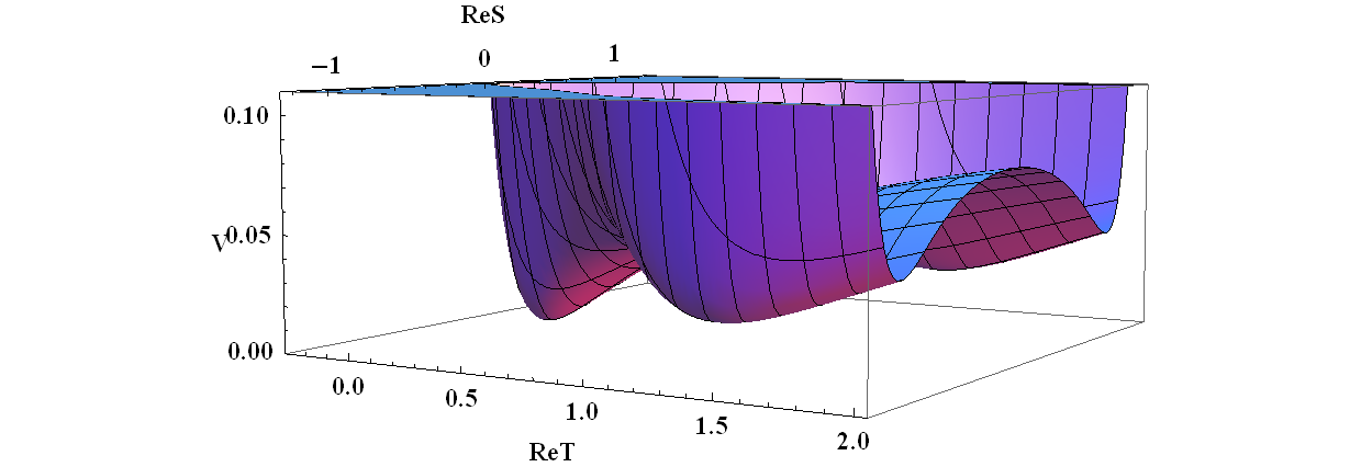
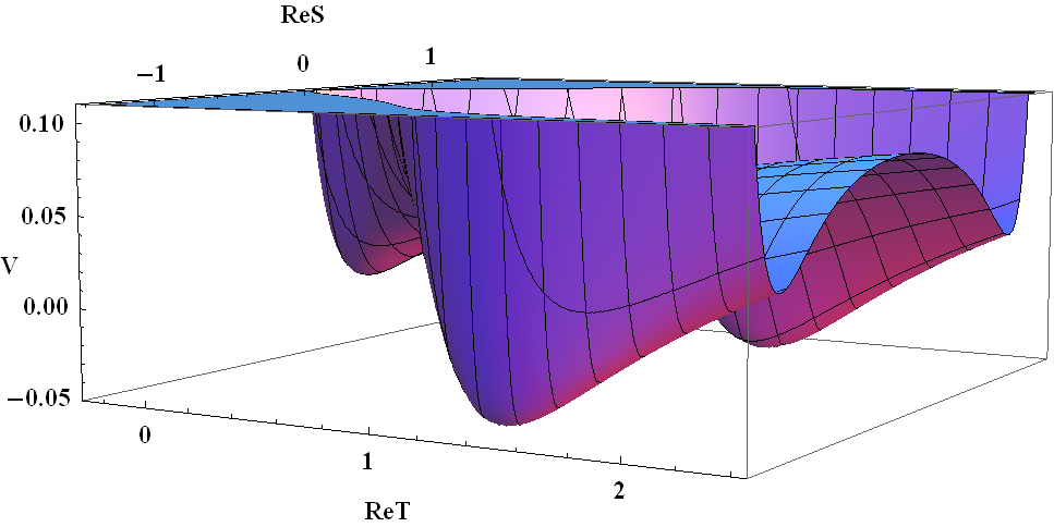
We can summarize the dependence of the vacuum structure of the R-symmetric models (for the relevant field space region) on the various $\zeta$ values

• •

  $\zeta>3.54\ \text{(Kallosh-Linde bound \cite[cite]{\@@bibref{Authors Phrase1YearPhrase2}{Kallosh:2013lkr}{\@@citephrase{(}}{\@@citephrase{)}}})}$: The $S$ field is always stabilized at $\langle S\rangle=0$ and the model has a single supersymmetric Minkowski vacuum for $\langle T\rangle=0$. For larger values of $\zeta$ the mass of the $S$-field increases and becomes bigger than the Hubble scale during inflation, therefore does not influence the dynamics.

• •

  $\zeta\gtrsim 1$: The model has two minima. The Minkowski one with $\langle S\rangle=\langle T\rangle=0$ which preserves supersymmetry and the local de Sitter one with $\langle|S|^{2}\rangle\sim M_{P}^{2}$ and $\langle T\rangle\sim M_{P}$, which breaks both supersymmetry and R-symmetry.

• •

  $\zeta=1\ \text{(Hindawi-Ovrut-Waldram critical value \cite[cite]{\@@bibref{Authors Phrase1YearPhrase2}{Hindawi:1995qa}{\@@citephrase{(}}{\@@citephrase{)}}})}$: The model has two degenerate Minkowski local minima. The trivial $\langle S\rangle=\langle T\rangle=0$ which preserves supersymmetry and the new one with $\langle|S|^{2}\rangle=M_{P}^{2}$ and $\langle T\rangle=\frac{4}{3}M_{P}$, which breaks both supersymmetry and R-symmetry with vanishing cosmological constant.

• •

  $\zeta\lesssim 1$: The model has two minima. The trivial Minkowski one $\langle S\rangle=\langle T\rangle=0$ which preserves supersymmetry and the global anti-de Sitter one with $\langle|S|^{2}\rangle\sim M_{P}^{2}$ and $\langle T\rangle\sim M_{P}$, which breaks both supersymmetry and R-symmetry.

• •

  $\zeta=0\ \text{(Cecotti critical value \cite[cite]{\@@bibref{Authors Phrase1YearPhrase2}{Cecotti:1987sa}{\@@citephrase{(}}{\@@citephrase{)}}})}$: The model has only one stable vacuum, the trivial Minkowski one which preserves supersymmetry. For $\zeta<0$ the model will in principle suffer from instabilities.

The above results have been collected in the following table 1.

In the previous section we saw higher curvature supergravity may have Minkowski vacua with broken supersymmetry, but this led to two drawbacks. Firstly, for a Minkowski vacuum one has to set $\zeta=1$ and therefore the same model can not describe a single field inflationary phase. Secondly, these vacua led to the spontaneous breaking of the R-symmetry, giving rise to the massless R-axion. Even for a de Sitter vacuum with a small cosmological constant these problems persist. In this section we introduce R-symmetry violating terms and we show how single field inflation and supersymmetry breaking can be realized in this class of models avoiding at the same time the R-axion massless mode.

References

- (1) S. J. Gates, M. T. Grisaru, M. Rocek and W. Siegel, “Superspace Or One Thousand and One Lessons in Supersymmetry,” hep-th/0108200.
- (2) J. Wess and J. Bagger, “Supersymmetry and supergravity,” Princeton, USA: Univ. Pr. (1992) 259 p
- (3) I. L. Buchbinder and S. M. Kuzenko, “Ideas and methods of supersymmetry and supergravity: Or a walk through superspace,” Bristol, UK: IOP (1998) 656 p
- (4) D. Z. Freedman and A. Van Proeyen, “Supergravity,” Cambridge, UK: Cambridge Univ. Pr. (2012) 607 p
- (5) D. H. Lyth and A. Riotto, “Particle physics models of inflation and the cosmological density perturbation,” Phys. Rept. 314, 1 (1999) [hep-ph/9807278].
- (6) A. A. Starobinsky, “A New Type of Isotropic Cosmological Models Without Singularity,” Phys. Lett. B 91, 99 (1980).
- (7) V. F. Mukhanov and G. V. Chibisov, “Quantum Fluctuation and Nonsingular Universe. (In Russian),” JETP Lett. 33, 532 (1981) [Pisma Zh. Eksp. Teor. Fiz. 33, 549 (1981)].
- (8) A. A. Starobinsky, “The Perturbation Spectrum Evolving from a Nonsingular Initially De-Sitter Cosmology and the Microwave Background Anisotropy,” Sov. Astron. Lett. 9, 302 (1983).
- (9) B. Whitt, “Fourth Order Gravity as General Relativity Plus Matter,” Phys. Lett. B 145, 176 (1984).
- (10) S. Ferrara, M. T. Grisaru and P. van Nieuwenhuizen, “Poincare and Conformal Supergravity Models With Closed Algebras,” Nucl. Phys. B 138, 430 (1978).
- (11) S. Cecotti, “Higher Derivative Supergravity Is Equivalent To Standard Supergravity Coupled To Matter. 1.,” Phys. Lett. B 190, 86 (1987).
- (12) S. Cecotti, S. Ferrara, M. Porrati and S. Sabharwal, “New Minimal Higher Derivative Supergravity Coupled To Matter,” Nucl. Phys. B 306, 160 (1988).
- (13) S. Cecotti, S. Ferrara and L. Girardello, “Massive Vector Multiplets From Superstrings,” Nucl. Phys. B 294, 537 (1987).
- (14) F. Farakos, A. Kehagias and A. Riotto, “On the Starobinsky Model of Inflation from Supergravity,” Nucl. Phys. B 876, 187 (2013) [arXiv:1307.1137].
- (15) S. Ferrara, R. Kallosh, A. Linde and M. Porrati, “Minimal Supergravity Models of Inflation,” Phys. Rev. D 88 (2013)085038, arXiv:1307.7696 [hep-th].
- (16) A. Van Proeyen, “Massive Vector Multiplets in Supergravity,” Nucl. Phys. B 162 (1980) 376.
- (17) S. Ferrara, R. Kallosh, A. Linde and M. Porrati, “Higher Order Corrections in Minimal Supergravity Models of Inflation,” JCAP 1311, 046 (2013) [arXiv:1309.1085 [hep-th]].
- (18) S. Ferrara, P. Fre and A. S. Sorin, “On the Topology of the Inflaton Field in Minimal Supergravity Models,” JHEP 1404, 095 (2014) [arXiv:1311.5059 [hep-th]].
- (19) S. Ferrara, P. Fre and A. S. Sorin, “On the Gauged Kähler Isometry in Minimal Supergravity Models of Inflation,” Fortsch. Phys. 62, 277 (2014) [arXiv:1401.1201 [hep-th]].
- (20) F. Farakos and R. von Unge, “Naturalness and Chaotic Inflation in Supergravity from Massive Vector Multiplets,” arXiv:1404.3739 [hep-th].
- (21) S. Ferrara and M. Porrati, “Minimal Supergravity Models of Inflation Coupled to Matter,” arXiv:1407.6164 [hep-th].
- (22) R. Kallosh, A. Linde and T. Rube, “General inflaton potentials in supergravity,” Phys. Rev. D 83, 043507 (2011) [arXiv:1011.5945 [hep-th]].
- (23) R. Kallosh and A. Linde, “Superconformal generalizations of the Starobinsky model,” JCAP 1306, 028 (2013) [arXiv:1306.3214 [hep-th]].
- (24) R. Kallosh and A. Linde, “Universality Class in Conformal Inflation,” JCAP 1307, 002 (2013) [arXiv:1306.5220 [hep-th]].
- (25) S. Ferrara, R. Kallosh and A. Van Proeyen, “On the Supersymmetric Completion of Gravity and Cosmology,” JHEP 1311, 134 (2013) [arXiv:1309.4052 [hep-th]].
- (26) S. V. Ketov and T. Terada, “Old-minimal supergravity models of inflation,” JHEP 1312, 040 (2013) [arXiv:1309.7494 [hep-th]].
- (27) R. Kallosh, A. Linde and D. Roest, “Universal Attractor for Inflation at Strong Coupling,” Phys. Rev. Lett. 112, no. 1, 011303 (2014) [arXiv:1310.3950 [hep-th]].
- (28) R. Kallosh, A. Linde and D. Roest, “Superconformal Inflationary -Attractors,” JHEP 1311, 198 (2013) [arXiv:1311.0472 [hep-th]].
- (29) S. Cecotti and R. Kallosh, “Cosmological Attractor Models and Higher Curvature Supergravity,” JHEP 1405, 114 (2014) [arXiv:1403.2932 [hep-th]].
- (30) I. Antoniadis, E. Dudas, S. Ferrara and A. Sagnotti, “The Volkov-Akulov-Starobinsky supergravity,” Phys. Lett. B 733, 32 (2014) [arXiv:1403.3269 [hep-th]].
- (31) S. Ferrara, A. Kehagias and A. Riotto, “The Imaginary Starobinsky Model,” Fortsch. Phys. 62, 573 (2014) [arXiv:1403.5531 [hep-th]].
- (32) K. Kamada and J. Yokoyama, “Topological inflation from the Starobinsky model in supergravity,” arXiv:1405.6732 [hep-th].
- (33) S. Ferrara and A. Kehagias, “Higher Curvature Supergravity, Supersymmetry Breaking and Inflation,” arXiv:1407.5187 [hep-th].
- (34) S. Ferrara, R. Kallosh and A. Linde, “Cosmology with Nilpotent Superfields,” arXiv:1408.4096 [hep-th].
- (35) M. Ozkan and Y. Pang, “ Extension of Starobinsky Model in Old Minimal Supergravity,” arXiv:1402.5427 [hep-th].
- (36) S. V. Ketov and A. A. Starobinsky, “Embedding ()-Inflation into Supergravity,” Phys. Rev. D 83, 063512 (2011) [arXiv:1011.0240 [hep-th]].
- (37) S. V. Ketov and A. A. Starobinsky, “Inflation and non-minimal scalar-curvature coupling in gravity and supergravity,” JCAP 1208, 022 (2012) [arXiv:1203.0805 [hep-th]].
- (38) S. V. Ketov and S. Tsujikawa, “Consistency of inflation and preheating in F(R) supergravity,” Phys. Rev. D 86, 023529 (2012) [arXiv:1205.2918 [hep-th]].
- (39) Y. Watanabe and J. Yokoyama, “Gravitational modulated reheating and non-Gaussianity in supergravity inflation,” Phys. Rev. D 87, no. 10, 103524 (2013) [arXiv:1303.5191 [hep-th]].
- (40) S. V. Ketov and T. Terada, “Inflation in Supergravity with a Single Chiral Superfield,” Phys. Lett. B 736, 272 (2014) [arXiv:1406.0252 [hep-th]].
- (41) S. V. Ketov and T. Terada, “Generic Scalar Potentials for Inflation in Supergravity with a Single Chiral Superfield,” arXiv:1408.6524 [hep-th].
- (42) J. Ellis, D. V. Nanopoulos and K. A. Olive, “No-Scale Supergravity Realization of the Starobinsky Model of Inflation,” Phys. Rev. Lett. 111, 111301 (2013) [arXiv:1305.1247 [hep-th]].
- (43) J. Ellis, D. V. Nanopoulos and K. A. Olive, “Starobinsky-like Inflationary Models as Avatars of No-Scale Supergravity,” JCAP 1310, 009 (2013) [arXiv:1307.3537].
- (44) J. Ellis, M. A. G. Garcia, D. V. Nanopoulos and K. A. Olive, “A No-Scale Inflationary Model to Fit Them All,” arXiv:1405.0271 [hep-ph].
- (45) J. Ellis and N. E. Mavromatos, “Inflation induced by Gravitino Condensation in Supergravity,” Phys. Rev. D 88, 085029 (2013) [arXiv:1308.1906 [hep-th]].
- (46) J. Alexandre, N. Houston and N. E. Mavromatos, “Starobinsky-type Inflation in Dynamical Supergravity Breaking Scenarios,” Phys. Rev. D 89, 027703 (2014) [arXiv:1312.5197 [gr-qc]].
- (47) J. Alexandre, N. Houston and N. E. Mavromatos, “Inflation via Gravitino Condensation in Dynamically Broken Supergravity,” arXiv:1409.3183 [gr-qc].
- (48) S. V. Ketov, “Starobinsky Model in N=2 Supergravity,” Phys. Rev. D 89, 085042 (2014) [arXiv:1402.0626 [hep-th]].
- (49) A. Ceresole, G. Dall’Agata, S. Ferrara, M. Trigiante and A. Van Proeyen, “A search for an inflaton potential,” Fortsch. Phys. 62, 584 (2014) [arXiv:1404.1745 [hep-th]].
- (50) P. Fré, A. S. Sorin and M. Trigiante, “The -map, Tits Satake subalgebras and the search for inflaton potentials,” arXiv:1407.6956 [hep-th].
- (51) K. Forger, B. A. Ovrut, S. J. Theisen and D. Waldram, “Higher derivative gravity in string theory,” Phys. Lett. B 388, 512 (1996) [hep-th/9605145].
- (52) D. Roest, M. Scalisi and I. Zavala, “Kähler potentials for Planck inflation,” JCAP 1311, 007 (2013) [arXiv:1307.4343].
- (53) N. Kitazawa and A. Sagnotti, “Pre-inflationary clues from String Theory?,” JCAP 1404, 017 (2014) [arXiv:1402.1418 [hep-th]].
- (54) C. Kounnas, D. Lüst and N. Toumbas, “ inflation from scale invariant supergravity and anomaly free superstrings with fluxes,” arXiv:1409.7076 [hep-th].
- (55) E. Kiritsis, “Asymptotic freedom, asymptotic flatness and cosmology,” JCAP 1311, 011 (2013) [arXiv:1307.5873 [hep-th]].
- (56) E. J. Copeland, C. Rahmede and I. D. Saltas, “Asymptotically Safe Starobinsky Inflation,” arXiv:1311.0881 [gr-qc].
- (57) A. Hindawi, B. A. Ovrut and D. Waldram, “Four-dimensional higher derivative supergravity and spontaneous supersymmetry breaking,” Nucl. Phys. B 476, 175 (1996) [hep-th/9511223].
- (58) A. Hindawi, B. A. Ovrut and D. Waldram, “Soft supersymmetry breaking induced by higher derivative supergravitation in the electroweak standard model,” Phys. Lett. B 381, 154 (1996) [hep-th/9602075].
- (59) S. Ferrara, A. Kehagias and M. Porrati, “Vacuum structure in a chiral modification of pure supergravity,” Phys. Lett. B 727, 314 (2013) [arXiv:1310.0399 [hep-th]].
- (60) T. Kugo and S. Uehara, “Conformal and Poincare Tensor Calculi in Supergravity,” Nucl. Phys. B 226, 49 (1983).
- (61) T. Kugo and S. Uehara, “ Superconformal Tensor Calculus: Multiplets With External Lorentz Indices and Spinor Derivative Operators,” Prog. Theor. Phys. 73, 235 (1985).
- (62) U. Lindstrom, A. Karlhede and M. Rocek, “The Component Gauges in Supergravity,” Nucl. Phys. B 191, 549 (1981).
- (63) D. Butter, “N=1 Conformal Superspace in Four Dimensions,” Annals Phys. 325, 1026 (2010) [arXiv:0906.4399 [hep-th]].
- (64) S. Ferrara and S. Sabharwal, “Structure of New Minimal Supergravity,” Annals Phys. 189, 318 (1989).
- (65) S. Ferrara, L. Girardello, T. Kugo and A. Van Proeyen, “Relation Between Different Auxiliary Field Formulations of Supergravity Coupled to Matter,” Nucl. Phys. B 223, 191 (1983).
- (66) S. Ferrara and M. Villasante, “Curvatures, Gauss-Bonnet and Chern-simons Multiplets in Old Minimal Supergravity,” J. Math. Phys. 30, 104 (1989).
- (67) U. Lindstrom and M. Rocek, “Constrained Local Superfields,” Phys. Rev. D 19, 2300 (1979).
- (68) F. Farakos and A. Kehagias, “Decoupling Limits of sGoldstino Modes in Global and Local Supersymmetry,” Phys. Lett. B 724, 322 (2013) [arXiv:1302.0866 [hep-th]].
- (69) S. P. de Alwis, “A Local Evaluation of Global Issues in SUSY breaking,” JHEP 1301, 190 (2013) [arXiv:1211.3913 [hep-th]].
- (70) R. Kallosh, A. Linde, B. Vercnocke and T. Wrase, “Analytic Classes of Metastable de Sitter Vacua,” arXiv:1406.4866 [hep-th].
- (71) I. Dalianis and Z. Lalak, “Cosmological vacuum selection and metastable susy breaking,” JHEP 1012, 045 (2010) [arXiv:1001.4106 [hep-ph]].
- (72) I. Dalianis and Z. Lalak, “Cosmological vacuum selection, metastable susy breaking and moduli,” Fortsch. Phys. 59, 1103 (2011).
- (73) A. Kehagias, A. M. Dizgah and A. Riotto, “Comments on the Starobinsky Model of Inflation and its Descendants,” Phys. Rev. D 89, 043527 (2014) [arXiv:1312.1155 [hep-th]].
- (74) P. A. R. Ade et al. [Planck Collaboration], “Planck 2013 results. XXII. Constraints on inflation,” arXiv:1303.5082 [astro-ph.CO].