Slow poisoning and destruction of networks: Edge proximity and its implications for biological and infrastructure networks

Considerable research has been done on the importance of various metrics in complex networks [1, 2, 3, 4]. The importance of nodes and remarkable effects of their targeted removal using various network metrics like betweenness and degree is now well known. In comparison, the role of edges has received less attention [5, 6, 7]. In this context, one may ask if it is possible to prognose situations where not even a single node is pruned from the network for a long time and yet tremendous damage is inflicted on it by selective targeting of specific edges. Indeed, as we show here, such a process might initially appear inconspicuous or even deceptively innocuous. Using a simple metric, which we call edge proximity, we are able to identify specific edges whose removal can slowly poison networks and silently wreak havoc in them. Furthermore, we show that ${\cal P}_{e}$ can be used to design strategies to consistently rupture networks into two nearly equal parts. Thus, this could eventually be far more destructive than currently available strategies for targeting network edges including those where rapid disconnection can be achieved due to detachment of small subgraphs from the parent network.

The most well-known edge-based measure, edge betweenness, ${\cal B}_{e}$, attempts to capture the frequency of an edge lying on the shortest paths between all pairs of vertices in a network [5, 6]. Edges with the highest ${\cal B}_{e}$ are most likely to lie between subgraphs, rather than inside them. Thus, targeting by node or edge betweenness ensures rapid disconnection of networks by a small number of deletions [8, 9].

Herein, we introduce a new edge-based network metric, edge proximity, ${\cal P}_{e}$. The ${\cal P}_{e}$ of an edge, $e\in{\cal E}$, is the inverse of the sum of its shortest distance $d(e,f)$, with every other edge, $f\in{\cal E}$, in a connected network, $\cal G(V,E)$. $\cal Vand\cal E$ denote the set of nodes and edges, respectively, in $\cal G$. $\cal N=|V|$ and $\cal M=|E|$ are the total number of nodes and edges in $\cal G$, respectively. ${\cal P}_{e}$ lends clues as to how close each edge is to every other edge in ${\cal G}$ through the shortest paths between them. Thus, for $e\in{\cal E}$,

The Average shortest path length, $\cal L_{G}$, is the average of all the shortest path lengths between any pair of nodes in ${\cal G}$ and is defined as,

The Diameter of ${\cal G}$ is defined as,

$d(s,t)$ being the shortest path from $s$ to $t$. From the definition of $\cal L_{G}$ and $\cal D$ it is clear that $\cal L_{G}$ and $\cal D$ become infinite when $\cal G$ becomes disconnected.

When edges are targeted by ${\cal B}_{e}$, the damage done to the network in the form of increases in $\cal L_{G}$ and $\cal D$ might initially seem to be greater. However, we observe here that ${\cal P}_{e}$ helps in identifying those crucial edges of undirected networks whose deletion ensures the highest increase in $\cal L_{G}$ and $\cal D$ in ${\cal G}$ (or its largest connected component, $\cal G^{\prime}$) compared to other methods of edge deletion. This appears to be true for both the first disconnection and well beyond. In fact, when targeting by ${\cal P}_{e}$ no node is disconnected from the network for a very long time. Here, we study the effect of various edge deletion strategies on real-world undirected networks like the E.U. and U.S. power grid network (PGNs) and the protein-protein interaction networks (PPINs) of S. cerevisiae and E. coli till the first disconnection. We also scrutinize the effect of these strategies, long after the first disconnection (till only about $30\%$ of the edges remain in $\cal G^{\prime}$), on various models like the Erdös-Rényi (ER) [10], Barabasi-Albert (BA) [11], and small-world (SW) [12, 13] networks. We also study a variety of directed biological networks, namely, the macaque brain network, the C. elegans neural network, and a number of food webs. We find that in each case ${\cal P}_{e}$ successfully provides meaningful biological information.

There have been lots of studies on disconnection of networks by malicious targeting. However, it is obvious that significant damage would be caused to the network when each disconnection causes the network to rupture into two nearly equal parts rather than having a small chunk disconnected from it. We demonstrate that ${\cal P}_{e}$ can be remarkably successful in consistently achieving this, compared to other methods of edge removal.

An edge with higher ${\cal P}_{e}$ should possess the potential to reach many other edges in directed networks. Of late, there has been considerable research on node controllability in networks [14, 15]. Switchboard dynamics (SBD) of edges has also been recently proposed to study edge controllability of directed networks and to identify the minimal set of driven edges [16]. We conclude by examining the natural potential that ${\cal P}_{e}$ possesses in the context of controllability of directed networks.

Figure 1 uses a toy example to illustrate the construction of a line graph $\cal L(G)$ from $\cal G$. The first step for creating $\cal L(G)$ is that every node in $\cal L(G)$ represents an edge in the original graph $\cal G$. An edge is drawn between any two nodes in $\cal L(G)$ if the corresponding edges in $\cal G$ share a common node. For directed graphs, an edge in $\cal L(G)$ represents a directed path of length $2$ in $\cal G$. Each node of $\cal L(G)$ is an edge of $\cal G$. Thus, ${\cal P}_{e},e\in\cal E$ can be obtained from closeness centrality of corresponding node in $\cal L(G)$.

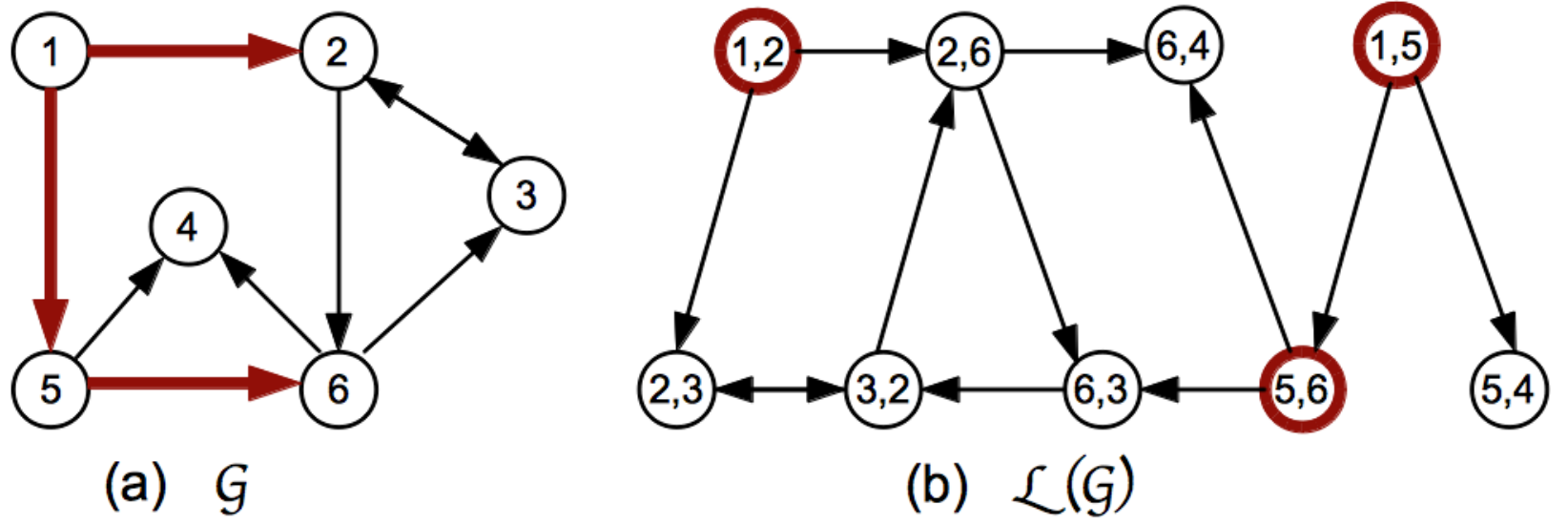
As is well known, the computational complexity of node closeness is ${\cal O~(|V|}~log~{\cal|V|+|E|})$. The number of nodes in $\cal L(G)$ is $\cal|E|$. The number of two-path lengths in $\cal G$ is the number of edges in $\cal L(G)$. Therefore the computational complexity for ${\cal P}_{e}$ is ${\cal O~(|E|}~log~{\cal|E|+|E|}^{2})$ and can be computed easily. All networks were analyzed here using NetworkX [17].

The very same edge-based metric, $\cal X(G)$, can be modelled with nodes involved in definition, as ${\cal X}_{1}{\cal(G)}$, or without nodes as ${\cal X}_{2}{\cal(G)}$. $|{\cal X}_{1}{\cal(G)}\sim{\cal X}_{2}{\cal(G)}|$ might not be very significant, especially when ${\cal G}$ is large. The computation time for ${\cal X}_{2}{\cal(G)}$ might be slightly longer than that for ${\cal X}_{1}{\cal(G)}$.

We investigate a number of edge deletion strategies which affect $\cal L_{G}$ and $\cal D$ in ${\cal G}$. The strategies adopted here consist of independently deleting successive edges: (i) with $max({\cal P}_{e})$, (ii) with $max({\cal B}_{e})$, (iii) connected to the node of the highest degree in ${\cal G}$ $[max({\cal K}_{e})]$, and, (iv) purely at random (${\cal R}_{e}$). To illustrate further, we construct four identical copies of ${\cal G(V,E)}$; $\{{\cal G}_{i}({\cal V}_{i},{\cal E}_{i})\},i\in\{1,2,3,4\}$. We then remove the edge with $max({\cal P}_{e})$, $max({\cal B}_{e})$, $max({\cal K}_{e})$, $e\in{\cal E}_{i},i\in\{1,2,3\}$, from ${\cal G}_{1}$, ${\cal G}_{2}$, ${\cal G}_{3}$, respectively. In case there is more than one edge with $max({\cal P}_{e})$, $max({\cal B}_{e})$, and $max({\cal K}_{e})$, we randomly choose one among them. We recalculate the values of ${\cal P}_{e}$, ${\cal B}_{e}$ and ${\cal K}_{e}$, $e\in{\cal E}_{i},i\in\{1,2,3\}$; for ${\cal G}_{1}$, ${\cal G}_{2}$, and ${\cal G}_{3}$, respectively. For all real-world networks studied here, we repeat this removal and recalculation process, until the first node is disconnected. In ${\cal G}_{4}$ edges are always deleted randomly.

We test these strategies for PGNs of the European Union [18] and United States [us-power] by recording change in $\cal L_{G}$ and $\cal D$ till the first node disconnection. As shown in Fig. 2, deletion of edges by ${\cal B}_{e}$ has a strong effect on the increase in $\cal D$ (and $\cal L_{G}$), initially. Random edge deletion does not lead a significant increase in $\cal D$ (and $\cal L_{G}$) of the PGNs. Similarly, targeting by $max({\cal K}_{e})$ does not lead to a significant increase in $\cal D$ (and $\cal L_{G}$), at least for the U.S. PGN. The most striking increase in $\cal D$ (and $\cal L_{G}$) is, however, seen for successive deletions using $max({\cal P}_{e})$. Thus ${\cal P}_{e}$ identifies specific edges whose existence is crucial for the network. Damage to these edges affects $\eta$, $\cal L_{G}$, and $\cal D$ significantly in PGNs.

We also calculate the efficiency, $\eta$, which is the average of the inverse of all shortest path lengths between any pair of nodes in $\cal G$ [19]:

Both E.U. and U.S. PGNs become disconnected by a small number of random edge deletions with insignificant loss of $\eta$, as shown in Fig. 3. Notably, connectedness is still maintained for both E.U. and U.S. PGNs when targeted by $max({\cal K}_{e})$. However, maximum loss of $\eta$ (and increase in $\cal D$ and $\cal L_{G}$) is observed when edges are targeted by $max({\cal P}_{e})$. Of course, loss of $\eta$ in the E.U. PGN is comparable for $max({\cal K}_{e})$ and $max({\cal P}_{e})$ strategies. However, it is not comparable for the U.S. PGN. Thus, in general, $max({\cal P}_{e})$ edges could be very different from $max({\cal K}_{e})$ edges.

We keep deleting edges even after the first node disconnection, until $\cal G^{\prime}$ contains only $30\%$ of the edges of $\cal G$, as shown in Fig. 4 for BA, ER and SW networks. Further edge deletions are not conducted because in very small graphs ${\cal P}_{e}$ loses its meaning, as every edge is usually quite close to most other edges. ${\cal D_{S}}$ fluctuates most in ER networks due to the larger number of disconnections. Effects due to ${\cal P}_{e}$ are higher in networks with higher clustering. Thus ${\cal P}_{e}$ should be important for many real-world networks.

Great harm can be caused to a network if it can be broken into two nearly equal parts at each disconnection rather than having a small part disconnected from it. As demonstrated in Figure. 5, for BA, ER, and SW networks, targeting by ${\cal P}_{e}$ can be a remarkably successful way to consistently achieve this outcome.

For all biological networks studied here, we scrutinise the biological significance of edges with the highest ${\cal P}_{e}$ and ${\cal B}_{e}$. For this purpose, we calculate

$\mu({\cal Q})$ is the mean and, $\sigma({{\cal Q}})$, the standard deviation of the ${\cal Q}$ distribution. For consistency, we restrict ourselves to the top $2\%$ of edges with ${\cal Z(Q})\geq 1$.

First, we observe the effect of edge deletion in $\cal G^{\prime}$ of yeast  [20] and E. coli [21] PPINs till first disconnection. As shown in Figs. 2 (c) and (d), removal of interactions by ${\cal P}_{e}$ increases $\cal L_{G}$ and $D$ of PPINs the most. In the E. coli PPIN, an essential protein, $60kDa$ chaperonin is consistently present at one end of ${\cal Z(P}_{e})\geq 1$ edges. This 60kDa protein exhibits a specific stress dependent co-expression with its connected proteins via these ${\cal Z(P}_{e})\geq 1$ edges [22], alike date hubs [23].

Tropic interactions and energy flow directions in food web networks (FWNs) are represented by directed edges from prey to predators [24]. The cascade of extinction and role of keystone species are well documented depending on the species- or node-based approach of FWNs [25, 26]. Tropic interactions or the edge-based approach might be beneficial for identifying important interactions in the FWN. Herein, we analyze three coral reef FWNs of Cayman Island, Cuba and Jamaica [27] and four FWNs in South Florida ecosystems [28, 29]. ${\cal B}_{e}$ and ${\cal P}_{e}$ identify different sets of edges for these FWNs. The root interactions of the dominator tree of corresponding FWNs [25, 30] are considered to be important interactions of primary consumers with producers or interactions with the outside environment. These are located at the initial positions in long food chains. Removal of these interactions may lead to secondary extinction of many species [25] or may stop the sending of input energy into the FWN from the outer environment [28, 29]. ${\cal P}_{e}$ seems to identify these root interactions correctly. ${\cal Z(P}_{e})\geq 1$ edges include such interactions as primary consumers interacting with planktonic bacteria, phytoplanton, or macrophytes and the environmental input to primary producers and epiphytes. ${\cal B}_{e}$ identifies other interactions between keystone species such as Diadema, bivalves, vertebrate detritus, meso-invertebrates, etc [31, 6, 32, 33, 34, 35, 36], successfully. Thus, many food chains possess ${\cal Z(B}_{e})\geq 1$ edges and their removal might hamper many tropic interactions [31].

There has been significant research on detecting emergent behavioral patterns from networks of interconnected neurons. Functional and structural aspects of neural networks are rather well studied in the case of the C. elegans network. The connectivity data have been obtained from reconstruction of electron microscopy [37]. To detect functionally and structurally important synapses, we analyze the network using ${\cal P}_{e}$ and ${\cal B}_{e}$. ${\cal Z(B}_{e})\geq 1$ identifies RME, AIB, RIA, RIF, AIM, and AEV synapses. These are ring motors and interneurons associated with thermotaxis and backward movement [38, 39, 40]. However, ${\cal Z(P}_{e})\geq 1$ identifies various synapses of AVEL which are solely associated with backward movement of C. elegans [38].

We also study the brain network of monkeys formed from connectivity data on macaque brain (CoCoMac data sets), where neural fibers connecting different portions of the brain are represented by directed edges [41]. Analyzing all neural connections by ${\cal B}_{e}$ and ${\cal P}_{e}$, we find that two rather different types of edges in hierarchical information processing pathways are identified by these two metrics. ${\cal Z(B}_{e})\geq 1$ identifies interactions which are essentially localized in the intermediate regions of the brain like the prefrontal cortex [42]. Interestingly, ${\cal Z(P}_{e})\geq 1$ corresponds to various connections from cortex to thalamus, frontal lobe and temporal lobe, which are the starting interactions of longer information processing pathways from the cortex to other regions of the brain [42].

Finally, under SBD of edge controllability, each node is conceived as acting similarly to a small switchboard-like device [16]. Nodes map the input signals of the inbound edges to the outbound edges. Figure. 1 depicts an example akin to Ref. [16]. The maximum matching algorithm is used for the line graph, $\cal L(G)$, constructed from the original network $\cal G=G(V,E)$ for identifying all possible sets of driven edges, ${\cal E}^{{}^{\prime}}=\{{\cal E}_{i}^{{}^{\prime}}:i\in{\mathbb{Z}_{+}}\}$, in $\cal G$ under SBD; ${\cal E}_{i}^{{}^{\prime}}\subseteq{\cal E}$. We calculate ${\cal P}_{e}$ and ${\cal B}_{e}$, $e\in{\cal E}$ in Fig. 1. Intuitively, edges with higher ${\cal P}_{e}$ could be driven edges for edge controllability under SBD. This is consistent with Table 1 where ${\cal P}_{e}>0$ for ${\cal E}_{1}^{{}^{\prime}}\in{\cal E^{\prime}}$. ${\cal E}_{2}^{{}^{\prime}}=\{(2,6),(3,2),(6,3)\}$ also shows ${\cal P}_{e}>0$, thus raising the question whether ${\cal E}_{2}^{{}^{\prime}}\in{\cal E^{\prime}}$? However, ${\cal E}_{2}^{{}^{\prime}}\in{\cal E}_{f}$, where $\{{\cal E}_{f}\}$ denotes all sets of edges participating in feedback loops of ${\cal G}$. Thus, ${\cal E}_{i}^{{}^{\prime}}\in\{{\cal E}_{f}\},i\in{\mathbb{Z}_{+}}\Longrightarrow{\cal E}_{i}^{{}^{\prime}}\notin{\cal E^{\prime}}$, because if ${\cal E}_{i}^{{}^{\prime}}\in\{{\cal E}_{f}\}$, ${\cal E}_{i}^{{}^{\prime}}$ is self-controllable. Again either of $(5,4)$, $(2,3)$, or $(6,4)$ is not a good driven edge because each of these edges can only control itself. We observe that ${\cal P}_{e}=0$ for them. This proof-of-concept example illustrates the potential utility of ${\cal P}_{e}$ to act as an index of edge control centrality of individual edges under SBD.

Even though infrastructure and biological networks have been examined in-depth in this paper, ${\cal P}_{e}$ would play a prominent role in most real-world and random networks, especially large ones. For very small networks, ${\cal P}_{e}$ becomes irrelevant because almost all edges are then mutually close. The slow poisoning effect due to ${\cal P}_{e}$ increases with clustering in undirected graphs. Therefore, ${\cal P}_{e}$ would be important in a wide variety of real-world networks. As with almost any other network metric, its importance would be rather limited in very dense graphs.

S.J.B. and S.S. thank CSIR, India and UGC, India respectively for financial support.

References

- [1] R. Albert and A.-L. Barabasi Rev. Mod. Phys. 74, 47 (2002).
- [2] M. E. J. Newman, Networks: An Introduction, Oxford Univ. Press, UK (2010).
- [3] V. Filkov et al., Europhys. Lett. 86, 28003 (2009)
- [4] S. Roy and V. Filkov, Phys. Rev. E 80, 040902(R) (2009)
- [5] M. E. Newman and M. Girvan, Phys. Rev. E 69, 026113 (2004).
- [6] M. Girvan, and M. E. Newman, Proc. Natl. Acad. Sci. (U.S.A) 99, 7821 (2002).
- [7] M. W. Berry et al., J Complex Networks 1, 93 (2013).
- [8] D. R. Wuellner, S. Roy and R. M. D’Souza, Phys. Rev. E 82, 056101 (2010).
- [9] S. Roy, Syst. Synth. Biol. 6 31 (2012).
- [10] P. Erdös and A. Rényi, Publicationes Mathematicae 6 290 (1959)
- [11] A.-L. Barabási and R. Albert, Science 286, 509 (1999).
- [12] D. Watts, S.H. Strogatz, Nature (London) 393 440 (1998).
- [13] S. Roy and S. M. Bhattacharjee, Phys. Lett. A 352, 13 (2006)
- [14] Y. Y. Liu, J. J. Slotine and A.L. Barabási, Nature (London) 473, 167 (2011).
- [15] S. J. Banerjee and S. Roy, arXiv: 1209.3737 (2012).
- [16] T. Nepusz and T. Vicsek, Nature Phys. 8, 568 (2012).
- [17] http://networkx.lanl.gov/
- [18] Q. Zhou and J. W. Bialek, IEEE Trans. on Power Systems 20, 782 (2005).
- [19] I. Vragović, E. Louis and A. Díaz-Guilera, Phys. Rev. E 71, 036122 (2005).
- [20] H.Jeong, S. P. Mason, A. L. Barabási and Z. N. Oltvai, Nature (London) 411 41 (2001).
- [21] J. M. Peregr-Alvarez, X. Xiong, C. Su and J. Parkinson, PLoS Comp. Biol. 5(10). (2009).
- [22] P. V. Viitanen, A. A. Gatenby and G. H. Lorimer, Protein Sci. 1, 363 (1992).
- [23] J. D. J. Han et al., Nature (London) 430, 88 (2004).
- [24] J. A. Dunne, R. J. Williams and N. D. Martinez, Proc. Natl. Acad. Sci. (U.S.A) 99, 12917 (2002).
- [25] S. Allesina and A. Bodini, J. Theo. Biol. 230, 351 (2004).
- [26] L. S. Mills, M. E. Soule and D. F. Doak, BioSci. 43, 219 (1993).
- [27] P. D. Roopnarine and R. Hertog, Dataset Papers in Ecology 2013, 857470 (2013).
- [28] R. E. Ulanowicz, J. J. Heymans and M. S. Egnotovich, FY 99: The Graminoid Ecosystem. Annual Report of the Biological Resources Division of the U.S. Geological Service (2000).
- [29] V. Batagelj and A. Mrvar, Pajek datasets. URL: http://vlado.fmf.uni-lj.si/pub/networks/data/ (2006).
- [30] E. Mones, L. Vicsek and T. Vicsek, PLoS ONE 7(3) e33799 (2012).
- [31] G. K. Bielmyer, K. V. Brix, T. R. Capo and M. Grosell, Aquat. Toxicol. 74, 254 (2005).
- [32] P. W. Sammarco, J. Exp. Mar. Biol. Ecol. 45, 245 (1980).
- [33] R. F. D. Dame, Ecology of Marine Bivalves: an Ecosystem Approach 2’nd Ed., CRC Press, NY (2011).
- [34] S. Z. Rahman and R. A. Khan, Ind. J Pharmacol. 38, 229 (2006).
- [35] J. Mauchline, The Biology of Calanoid Copepods, Advances in Marine Biology, 33, Eds. Blaxter, J. H., Southward and A. J, Tyler, P. A., Acad. Press London (1998).
- [36] R. F. Dame and T. C. Prins, Aquat. Ecol. 31, 409 (1997).
- [37] J. G. White, E. Southgate, J. N. Thomson and S. Brenner, Phil. Trans. Royal Soc. London B 314, 1(1986).
- [38] D. L. Riddle, T. Blumenthal, B. J. Meyer and J. R. Preiss, Introduction to C. elegans – C. elegans II, Cold Spring Harbor Lab. Press, NY (2’nd Ed.) (1997).
- [39] T. Wakabayashi, I. Kitagawa and R. Shingai, Neurosci. Res. 50, 103 (2004).
- [40] N. Ohnishi et al., EMBO journal 30, 1376 (2011).
- [41] K. E. Stephan et al., Phil. Trans. Royal Soc. London B 356, 1159 (2001).
- [42] D. S. Modha and R. Singh, Proc. Natl. Acad. Sci. (U.S.A) 107, 13485 (2010).