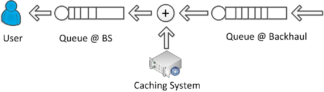
Denote $\mathcal{B}$ as the set of BSs including both MBSs and SCBSs and $\mathcal{A}$ as the coverage area of all BSs. Here, a BS refers to either a MBS or a SCBS. Since BSs are equipped with cache, users’ data requests can be fulfilled by the cache system if the requested content is cached; otherwise, the requested content is retrieved from Internet. Retrieving contents from Internet generates traffic loads in a BS’s backhaul. Therefore, we model the traffic delivery process as a queuing system as shown in Fig. 2.

The performance of a cache system is commonly evaluated based on the cache hit ratio that is defined as the ratio between the number of cache hits and the total requests observed over a period of time [24]. Many analytical models have been proposed to estimate the hit ratio of a cache system and various content caching strategies have been designed to optimize the performance of cache systems [24, 25, 26, 27, 28]. Thus, in the paper, we assume that the hit ratio of a cache system in a BS can be estimated for the time duration of one user association process and denote $0\leq\alpha_{j}\leq 1$ as the hit ratio of the cache system in BS $j$. Note that how to optimize and estimate the hit ratio is out of the scope of this paper.

Let a mobile user at location $x$ associate with BS $j$. We assume that the traffic arrives at BS $j$’s backhaul toward the user according to a Poisson process with the arrival rate equaling to $\tilde{\lambda}(x)$, and the traffic loads per arrival (packet sizes per arrival) have an exponential distribution with the average traffic load of $\nu(x)$. We assume that the users associated with BS $j$ are uniformly distributed in its coverage area and the traffic arrival processes are independent. For presentation simplicity, we further assume that no users share the same locations, i.e., only one user at location $x$. Since the traffic arrival toward a location is a Poisson process, the traffic arrival in BS $j$’s backhaul, which is the sum of the traffic arrivals from its coverage area, is also a Poisson process. Although BSs may adopt different access technologies as their backhaul, it is reasonable to assume the expected data rates of the backhaul are constant in the time duration of one user association process [21]. Since the traffic load per arrival follows an exponential distribution, the traffic delivery time (service time) of the backhaul is also an exponential distribution. Therefore, the traffic delivery in backhaul simply realizes an M/M/1 queuing system.

Denoting $R_{j}$ as the average data rate of BS $j$’s backhaul. To fulfill the traffic demand of the user at location $x$ , the required service time in BS $j$’s backhaul is

$$\tilde{\gamma}(x)=\frac{\nu(x)}{R_{j}}.$$

(1)

The average traffic load density generated by a user at location $x$ in BS $j$’s backhaul is

$$\tilde{\varrho}_{j}(x)=\frac{\tilde{\lambda}(x)\nu(x)\eta_{j}(x)}{R_{j}}$$

(2)

Here, $\eta_{j}(x)=\{0,1\}$ is an indicator function. If $\eta_{j}(x)=1$, the user at location $x$ is associated with BS $j$; otherwise, the user is not associated with BS $j$. Since mobile users are uniformly distributed in the area, the traffic load in BS $j$’s backhaul can be expressed as

$$\tilde{\rho}_{j}=\int_{x\in\mathcal{A}}\tilde{\varrho}_{j}(x)dx.$$

(3)

According to the properties of the M/M/1 queue [29], the average waiting time for traffic load $\nu(x)$ in BS $j$’s backhaul is

$$\tilde{W}_{j}(x)=\frac{\tilde{\rho}_{j}\nu(x)}{R_{j}(1-\tilde{\rho}_{j})}.$$

(4)

Denote $\tilde{\mu}_{j}(x)$ as the latency ratio that measures how much time a user at location $x$ must be sacrificed in waiting for per unit service time in BS $j$’s backhaul.

$$\tilde{\mu}_{j}(x)=\frac{\tilde{W}_{j}(x)}{\tilde{\gamma}(x)}=\frac{\tilde{\rho}_{j}}{1-\tilde{\rho}_{j}}.$$

(5)

Since $\tilde{\mu}_{j}(x)$ only depends on the traffic load in BS $j$’s backhaul, all the users associated with BS $j$ have the same latency ratio. Thus, we define

$$\tilde{\mu}_{j}(\tilde{\rho_{j}})=\frac{\tilde{\rho_{j}}}{1-\tilde{\rho_{j}}}$$

(6)

as the latency ratio of BS $j$’s backhaul. A smaller $\tilde{\mu}_{j}(\tilde{\rho_{j}})$ indicates that BS $j$’s backhaul introduces less latency to its associated users.

According to Burke’s Theorem [29], the traffic departure process at a BS’s backhaul is a Poisson process with average departure rate equaling to the average traffic arrival rate. Therefore, the average traffic arrival rate in BS $j$ toward a user at location $x$ equals to $\tilde{\lambda}(x)$. Since the hit ratio of BS $j$’s cache system is $\alpha_{j}$, the data traffic from the backhual accounts for $(1-\alpha_{j})$ of the total traffic load toward the user at location $x$. Therefore, the average traffic arrival rate in BS $j$ toward the user at location $x$ is

$$\lambda(x)=\frac{\tilde{\lambda}(x)}{(1-\alpha_{j})}.$$

(7)

Since $\alpha_{j}$ is assumed to be a constant during one user association process, the traffic arrival process toward the user at location $x$ is a Poisson process. In BS $j$, users at different locations may have different data rates depending on channel conditions. When associating with BS $j$, the user’s data rate, $r_{j}(x)$, can be generally expressed as a logarithmic function of the perceived SINR, $SINR_{j}(x)$, according to the Shannon-Hartley Theorem [6],

$$r_{j}(x)=log_{2}(1+SINR_{j}(x)).$$

(8)

Here,

$$SINR_{j}(x)=\frac{P_{j}g_{j}(x)}{\sigma^{2}+\sum_{k\in\mathcal{B},k\neq j}P_{k}g_{k}(x)}.$$

(9)

Here, $P_{j}$ is the transmission power of BS $j$, and $\sigma^{2}$ denotes the noise power level. Since the users’ data rate is generally distributed, the service time in BS $j$ follows a general distribution. Therefore, a BS’s downlink transmission process realizes a M/G/1 processor sharing (PS) queue, in which multiple users share the BS’s downlink radio resource [29].

In mobile networks, various downlink scheduling algorithms have been proposed to enable proper sharing of the limited radio resource in a BS. According to the scheduling algorithm, users may be assigned different priorities on sharing the radio resource. For analytical simplicity, we assume that mobile users are served based on the round robin (RR) fashion. Then, the average traffic load density at location $x$ in BS $j$ is calculated as

$$\varrho_{j}(x)=\frac{\lambda(x)\nu(x)\eta_{j}(x)}{r_{j}(x)}$$

(10)

The traffic load in BS $j$ can be expressed as

$$\rho_{j}=\int_{x\in\mathcal{A}}\varrho_{j}(x)dx.$$

(11)

This value of $\rho_{j}$ indicates the fraction of time during which BS $j$ is busy. To fulfill the traffic demand of a user located at $x$, the required service time in BS $j$ is

$$\gamma(x)=\frac{\nu(x)}{r_{j}(x)}.$$

(12)

Since the traffic delivery process in a BS realizes a M/G/1-RR queue, the average traffic delivery time for the user in BS $j$ [29] is

$$T_{j}(x)=\frac{\nu(x)}{r_{j}(x)(1-\rho_{j})}.$$

(13)

The average waiting time for traffic load $\nu(x)$ in BS $j$ is

$$W_{j}(x)=T_{j}(x)-\gamma(x)=\frac{\rho_{j}\nu(x)}{r_{j}(x)(1-\rho_{j})}.$$

(14)

Denote $\mu_{j}(x)$ as the latency ratio of BS $j$ for a user at location $x$.

$$\mu_{j}(x)=\frac{W_{j}(x)}{\gamma(x)}=\frac{\rho_{j}}{1-\rho_{j}}.$$

(15)

$\mu_{j}(x)$ only depends on the traffic load in BS $j$. Therefore, all the users associated with BS $j$ have the same latency ratio. Thus, we define

$$\mu_{j}(\rho_{j})=\frac{\rho_{j}}{1-\rho_{j}}$$

(16)

as the latency ratio of BS $j$. A smaller $\mu_{j}(\rho_{j})$ indicates that BS $j$ introduces less latency to its associated users. In this paper, we use $\mu_{j}$ and $\tilde{\mu}_{j}$ to reflect the traffic delivery latency in BS $j$ and its backhual, respectively, we adopt $\mu_{j}(\rho_{j})+\tilde{\mu}_{j}(\tilde{\rho}_{j})$ as the QoS model that indicates the latency of delivering traffic through BS $j$.

In the network, BSs have their own renewable energy systems (solar panels) for generating electricity. Meanwhile, BSs are connected with the power grid for electricity supplies. Thus, BSs are powered by hybrid energy sources: green power and brown power. A BS consumes brown power when green power is not sufficient. We assume that the green power systems in MBSs have a higher energy generation capacity than that of SCBSs because MBSs usually consume more energy than SCBSs owing to a relatively large coverage area. Fig. 3 shows a reference design of a hybrid energy powered BS [14].

The charge controller optimizes the green power utilization based on the solar power intensity, the power consumption of BSs, and prices of energy drawn from the power grid. Based on the optimization, the charge controller determines how much green power should be utilized to power a BS during a specific time period, e.g., the time duration between two consecutive traffic load balancing procedures [16]. In this paper, we focus on how to balance traffic load among BSs to reduce the traffic delivery latency as well as the brown power consumption within the duration of a traffic balancing procedure. Investigating how to optimize the green power utilization over the time horizon is out of the scope of this paper. Thus, we assume that the amount of available green power for powering a BS within the duration of one user association process is given by the charge controller as a constant [16]. This assumption is reasonable because the traffic load balancing process is at a time scale of several minutes [6] while solar power generation is usually modeled at a time scale of a hour [30]. Denote $e_{j}$ as the amount of green power for powering BS $j$ in a user association procedure. If BS $j$’s power consumption is larger than $e_{j}$, the BS consumes brown power. Otherwise, we simply model the BS’s brown power consumption are zero¹¹ 1 We do not consider the redistribution of the residual green power in our model, which is out of the scope of this paper..

The BS’s power consumption includes two parts: the static power consumption and the dynamic power consumption [31]. The static power consumption is the power consumption of a BS without carrying any traffic load. The dynamic power consumption refers to the additional power consumption incurred by traffic load in the BS, which can be well approximated by a linear function of the traffic load [31]. Denote $p^{s}_{j}$ as BS $j$’s static power consumption. Then, BS $j$’s power consumption is

$$p_{j}=\beta_{j}\rho_{j}+p^{s}_{j}.$$

(17)

Here, $\beta_{j}$ is the load-power coefficient that reflects the relationship between BS $j$’s traffic load and its dynamic power consumption. The BS power consumption model can be adjusted to model the power consumption of either MBSs or SCBSs by incorporating and tweaking the static power consumption and the load-power coefficient [16]. The BS $j$’s brown power consumption is

$$p^{b}_{j}=\max{(p_{j}-e_{j},0)}.$$

(18)

In determining the user association, the network aims to not only enhance the network QoS by reducing the traffic delivery latency but also reduce the brown power consumption by improving the green power utilization. Owing to the dynamics of the data traffic and green power, the user association that minimizes the traffic delivery latency does not necessarily maximize the green power utilization. Thus, the traffic load balancing problem strives for a trade-off between the traffic delivery latency and the brown power consumption.

According to E.q. (18), brown power is consumed only when green power is not sufficient ($e_{j}<p_{j}$). Given $e_{j}$, the maximum traffic load can be supported by green power in BS $j$ is

$$\hat{\rho}_{j}=max(0,min(\frac{e_{j}-p_{j}^{s}}{\beta_{j}},1-\epsilon)).$$

(19)

Here, $\epsilon$ is an arbitrary small positive constant to guarantee $0\leq\hat{\rho}_{j}<1$. Define $\hat{\rho}_{j}$ as BS $j$’s green traffic capacity. When BS $j$’s traffic load is larger than $\hat{\rho}_{j}$, BS $j$ consumes brown power. In this case, it is desirable to offload data traffic from BS $j$ to alleviate its brown power consumption. Let

$$\bar{\rho}_{j}=\rho_{j}-\hat{\rho}_{j}.$$

(20)

When $\bar{\rho}_{j}>0$, BS $j$’s traffic load is larger than its green power capacity and thus it is desirable to offload traffic from BS $j$ to save brown power; when $\bar{\rho}_{j}<0$, it is desirable to let BS $j$ carry additional traffic load to enhance the usage of green power and thus reduce other BSs’ brown power consumption. However, balancing traffic purely based on the energy consumption may lead to heavy traffic congestion that increases the traffic delivery latency in BSs. In order to strive a balance, we introduce latency weights for individual BSs. Denote

$$w_{j}(\rho_{j})=e^{\kappa\bar{\rho}_{j}}$$

(21)

as BS $j$’s latency weight. $\kappa\geq 0$ is a system parameter that adjusts the value of the latency weight.

Aiming to save brown power as well as to reduce the traffic delivery latency of the network, the traffic load balancing problem is formulated as

	$\displaystyle\min_{\boldsymbol{\eta}}$		$\displaystyle\sum_{j\in\mathcal{B}}w_{j}(\rho_{j})(\mu_{j}(\rho_{j})+\tilde{\mu}_{j}(\tilde{\rho}_{j}))$		(22)
	$\displaystyle subject\;to:$		$\displaystyle\rho_{j}=\int_{x\in\mathcal{A}}\frac{\lambda(x)\nu(x)\eta_{j}(x)}{r_{j}(x)}dx,$		(23)
			$\displaystyle\tilde{\rho}_{j}=\int_{x\in\mathcal{A}}\frac{\tilde{\lambda}(x)\nu(x)\eta_{j}(x)}{R_{j}}dx,$
			$\displaystyle 0\leq\rho_{j}\leq 1-\epsilon,$
			$\displaystyle 0\leq\tilde{\rho}_{j}\leq 1-\epsilon,$
			$\displaystyle\eta_{j}(x)=\{0,1\},\forall j\in\mathcal{B},x\in\mathcal{A}.$

Here, $\boldsymbol{\eta}=\{\boldsymbol{\eta}_{j}|j\in\mathcal{B}\}$ and $\boldsymbol{\eta}_{j}=\{\eta_{j}(x)|x\in\mathcal{A}\}$. Based on the formulation, if BS $j$ has sufficient green power ($\tilde{\rho_{j}}\geq\rho_{j}$), ${0<w_{j}(\rho_{j})\leq 1}$; otherwise, $w_{j}(\rho_{j})>1$. A large latency weight grants a BS a high priority in minimizing Eq. (22) as compared with those of the BSs having a small latency weight. In other words, a large latency weight grants a BS a high priority in offloading traffic. As compared with $w_{j}(\rho_{j})\leq 1$, $w_{j}(\rho_{j})>1$ enables BS $j$ to achieve a smaller latency ratio. Since $\frac{d\mu_{j}(\rho_{j})}{d\rho_{j}}>0$ and $\frac{d\tilde{\mu}_{j}(\tilde{\rho}_{j})}{d\tilde{\rho}_{j}}>0$, a small latency ratio indicates that BS $j$ carries a lighter traffic load, which is desirable for a BS which is consuming brown power ($w_{j}(\rho_{j})\leq 1$). $\kappa$ is a system parameter that enables the network dynamically controlling the trade-off between the brown power consumption and the traffic delivery latency.

The traffic load balancing procedures can be implemented in either a distribute or a centralized fashion [16]. For a distributed traffic load balancing, users select their serving BSs based on the operating parameters, e.g., traffic loads and data rates received from BSs. This will incur several interactions between BSs and users for updating the operating parameters and BS selections, respectively. For a centralized traffic load balancing scheme, the network collects the operating status information from both BSs and users, and determines the user association for individual users. A distributed traffic load balancing scheme can be implemented in a centralized fashion by leveraging virtualization techniques [16]. Thus, we propose a distributed traffic offloading procedure that includes four phases. The first phase is the initial user association and network utility measurements. When entering the network, a user simply attaches to any BS to retrieve network utility information. According to the initial user association, BSs measure their traffic load and estimate the traffic load in their backhaul. Based on the measurements, BSs, in the second phase, advertise their network utility information. Denote $\psi(\boldsymbol{\eta})=\sum_{j\in\mathcal{B}}w_{j}(\rho_{j})(\mu_{j}(\rho_{j})+\tilde{\mu}_{j}(\tilde{\rho}_{j}))$. In the third phase, the users select their serving BSs according to the advertised network utility information and the downlink data rates to minimize $\psi(\boldsymbol{\eta})$. In the fourth phase, the BSs and users iteratively update their network utilities (the second phase) and BS selections (the third phase), respectively, until the user association converges.

The network utility aware user association scheme consists of a user side algorithm and a BS side algorithm. The user side algorithm based on the network utility advertisement selects the optimal serving BS for individual users while the BS side algorithm updates individual BSs’ network utility advertisements based on the user association. In designing the network utility aware user association scheme, we make the following assumptions:

1. 1.

   We assume that the time scale of the traffic arrival and departure process is faster relative to that of BSs in advertising their network utility information. That is to say, BSs advertise their network utility information after the system exhibits the stationary performance.

2. 2.

   We assume that the green power generation rate is consistent during the time period of establishing a stable user association [23].

3. 3.

   We assume that all the BSs are synchronized and advertise their network utility simultaneously and the system parameter $\kappa$ does not change during one user association process.

4. 4.

   We assume that a BS’s cache hit ratio is constant within the duration of one user association.

The feasible set for the traffic load balancing problem in Eq. (22) is

	$\displaystyle\mathcal{F}=\{$	$\displaystyle\boldsymbol{\eta}|0\leq\tilde{\rho}_{j}\leq 1-\epsilon,$
		$\displaystyle 0\leq\rho_{j}\leq 1-\epsilon,\;\sum_{j\in\mathcal{B}}\eta_{j}(x)=1,$
		$\displaystyle\eta_{j}(x)=\{0,1\},\;\forall j\in\mathcal{B},\;\forall x\in\mathcal{A}\}$		(24)

Since $\eta_{j}(x)=\{0,1\}$, $\psi(\boldsymbol{\eta})$ is not continuous differentiable. In order to derive the user side algorithm and the BS side algorithm for the NUA traffic load balancing scheme, we relax the feasible set by letting $0\leq\eta_{j}(x)\leq 1$. Then, the relaxed feasible set is

	$\displaystyle\tilde{\mathcal{F}}=\{$	$\displaystyle\boldsymbol{\eta}|0\leq\tilde{\rho}_{j}\leq 1-\epsilon,$
		$\displaystyle 0\leq\rho_{j}\leq 1-\epsilon,\;\sum_{j\in\mathcal{B}}\eta_{j}(x)=1,$
		$\displaystyle 0\leq\eta_{j}(x)\leq 1,\;\forall j\in\mathcal{B},\;\forall x\in\mathcal{A}\}$		(25)

After presenting the NUA traffic load balancing scheme, we will prove that the proposed scheme achieves an optimal user association in the feasible set of the traffic load balancing problem.

We define the time interval between two consecutive network utility advertisements as a time slot. Let $\eta_{j}^{k}(x)$ denote whether a user at location $x$ associates with BS $j$ in the $k$th time slot. Denote $\rho_{j}(k)$ and $\tilde{\rho}_{j}(k)$ as the traffic load in BS $j$ and its backhaul in the $k$th time slot, respectively. Let

	$\displaystyle\phi_{j}(k)$	$\displaystyle=\frac{d\psi(\boldsymbol{\eta})}{d\eta_{j}(x)}$
		$\displaystyle=\frac{\lambda(x)\nu(x)}{r_{j}(x)}e^{\kappa(\rho_{j}(k)-\hat{\rho}_{j})}(\frac{\kappa\rho_{j}(k)}{1-\rho_{j}(k)}+\frac{\kappa\tilde{\rho}_{j}(k)}{1-\tilde{\rho}_{j}(k)}+\frac{1}{(1-\rho_{j}(k))^{2}})$
		$\displaystyle+\lambda(x)\nu(x)e^{\kappa(\rho_{j}(k)-\hat{\rho}_{j})}\frac{1-\alpha_{j}}{R_{j}(1-\tilde{\rho}_{j}(x))^{2}}.$		(26)

Define

$$\theta^{a}_{j}(k)=e^{\kappa(\rho_{j}(k)-\hat{\rho}_{j})}(\frac{\kappa\rho_{j}(k)}{1-\rho_{j}(k)}+\frac{\kappa\tilde{\rho}_{j}(k)}{1-\tilde{\rho}_{j}(k)}+\frac{1}{(1-\rho_{j}(k))^{2}})$$

(27)

and

$$\theta^{b}_{j}(k)=e^{\kappa(\rho_{j}(k)-\hat{\rho}_{j})}\frac{1-\alpha_{j}}{R_{j}(1-\tilde{\rho}_{j}(x))^{2}}.$$

(28)

Since $\theta^{a}_{j}(k)$ and $\theta^{b}_{j}(k)$ are calculated based on BS $j$’s network utility, we define $\theta^{a}_{j}(k)$ and $\theta^{b}_{j}(k)$ as the network utility information advertised by BS $j$ in the $k$th time slot.

In this subsection, we prove the convergence and the optimality of the proposed NUA traffic load balancing scheme. Since users select serving BSs based on BSs’ network utility advertisements, the user association converges when BSs’ network utility advertisements are stablilized. A BS’s network utility advertisements are determined by its intermediate traffic loads in the BS and its backhaul. On calculating the intermediate traffic loads, the intermediate user association is the only variable. Therefore, when the intermediate user association converges, the intermediate traffic load is stabilized and so are the network utility advertisements. Therefore, we first prove any BS’s network utility advertisements are stabilized by proving that its intermediate user association converges and then show that the user association based on the stabilized network utility advertisements minimizes $\psi(\boldsymbol{\eta})$.

Let $\bar{\boldsymbol{\eta}}^{k}=\{\bar{\boldsymbol{\eta}}^{k}_{j}|j\in\mathcal{B}\}$ and $\triangle\bar{\boldsymbol{\eta}}^{k}=\bar{\boldsymbol{\eta}}^{k}-\bar{\boldsymbol{\eta}}^{k-1}$.

Denote $\bar{\boldsymbol{\eta}}^{*}$ as the optimal intermediate user association.

The system parameter, $\kappa$, controls the tradeoff between the green power utilization and the traffic delivery latency. When $\kappa=0$, $w_{j}(\rho_{j})=1$. In this case, the green power utilization is not modeled in the objective function. Thus, the NUA traffic load balancing scheme determines the user association based only on the traffic delivery latency. As $\kappa$ increases, the awareness of green power utilization in determining the user association enhances. In other words, with a larger $\kappa$, the green power utilization plays a more important role in determining the user association. If $\kappa$ is large enough, the NUA traffic load balancing scheme achieves a user association that approximates the user association that only cares about the green power utilization.

We set up system level simulations to investigate the performance of the NUA traffic load balancing scheme for the downlink traffic load balancing in backhaul constrained SCNs. In the simulation, three MBSs and seven SCBSs are randomly deployed in a $2000m\times 2000m$ area. The total bandwidth is 10 $MHz$ and the frequency reuse factor is one. The channel propagation model is based on COST 231 Walfisch-Ikegami [32]. The channel model and parameters are summarized in Table I. Here, $PL_{MBS}$ and $PL_{SCBS}$ are the path loss between the users and MBSs and SCBSs, respectively. $d$ is the distance between users and BSs. The transmit power of an MBS and an SCBS are 43 $dBm$ and 33 $dBm$, respectively.

The static power consumptions of an MBS and an SCBS are 750 $W$ and 37 $W$, respectively [31]. The load-power coefficients of the MBS and the SCBS are 500 and 4, respectively [31]. The solar cell power efficiency is $17.4\%$ [33]. We assume that the weather condition is the standard condition which specifies a temperature of 25 ${}^{o}C$, an irradiance of 1000 $W/m^{2}$, and an air mass of 1.5 spectrum [34]. Thus, the green power generation rate is 174 $W/m^{2}$. The solar panel sizes are randomly selected but ensure the green power generation capacity of MBSs from 750 $w$ to 1300 $w$ while that of SCBSs from 37 $w$ to 48 $w$. BSs’ energy-latency coefficients are set to be the same. In the simulation, the average data rate of SCBSs’ backhaul is $5$ Mbps. The hit ratio³³ 3 The cache hit ratio is randomly selected from 0.1 to 0.3. For the analytical simplicity, we fix the hit ratio of BSs in the simulations. of BSs’ cache system is shown in Table II.

In the simulations, we investigate the performance of traffic load balancing schemes with different levels of network utility awareness. The network utilities considered in this paper are green power, the traffic delivery latency in BSs, the traffic delivery latency in backhaul, and the cache hit ratio. We implement three traffic load balancing schemes in the simulations. The first scheme is vGALA [16]. Adapting the parameters of vGALA ($\kappa$ and $\theta$), we realize the three traffic load balancing schemes: 1) BS latency aware, 2) green power aware, and 3) BS latency and green power aware. The second scheme is the NUA traffic load balancing scheme that simulates four traffic load balancing schemes: 1) BS latency and backhaul latency aware, 2) BS latency, backhaul latency and cache hit ratio aware, 3) BS latency, backhaul latency and green power aware, and 4) all network utilities aware. For the NUA scheme, when $\alpha_{j}=0,\;\forall j\in\mathcal{B}$, a BS estimates the traffic delivery latency in backhaul purely based on the traffic arrival rates in the BS. In fact, if the cache system is considered, the traffic load in backhaul should be less than that in the BS. Therefore, the NUA scheme with $\alpha_{j}=0,\;\forall j\in\mathcal{B}$, simulates the cache unaware traffic load balancing scheme. The third scheme is the data rate bias (DRB) scheme [19]. In the implementation, we assume that BSs in the same tier have the data rate bias. MBSs are in the first tier while SCBSs are in the second tier. In the data rate bias scheme, a user selects the serving BS to maximize the biased data rate. The data rate bias of an MBS is set to one. We vary the data rate bias of an SCBS to investigate the performance of the scheme. We set $\psi(\boldsymbol{\eta})$ as the performance metric for selecting the optimal data rate bias. Thus, the implemented DRB scheme is aware of all network utilities and is referred to as DRB-NU (the data rate bias with network utility awareness). The network utility awareness of the schemes with different settings are shown in Table III.

Fig. 4 shows the convergence of the NUA scheme and its energy-latency tradeoff with different $\kappa$. Fig. 4(a) shows the the value of $\psi(\boldsymbol{\eta})$ converges with less than 100 iterations, and so do the traffic delivery latency (Fig. 4(b)) and the brown power consumption (Fig. 4(c)). Figs. 4(b) and 4(c) show the energy-latency tradeoff. As $\kappa$ increases, the network emphasizes the green power utilization in determining the user association. As a result, with a large $\kappa$, e.g., $\kappa=7$, the network consumes less brown power at the cost of introducing additional traffic delivery latency. The vGALA with a large $\kappa$ and $\theta$, e.g., $\kappa=6$ and $\theta=1$, realizes the user association that is only aware of green power utilization [16]. Fig. 4(c) shows that as $\kappa$ increases, the performance of the NUA scheme in terms of the brown power consumption approaches that of the traffic load balancing scheme that optimizes the green power utilization (only aware of green power utilization).

Fig. 5 shows the performance of the NUA scheme versus different solar panel efficiency. Fig. 5(b) shows that the brown power consumption reduces as the solar panel efficiency increases. This is because a higher solar panel efficiency enables solar panels to generate a larger amount of electricity and thus lessen the brown power consumption. As shown in Fig 5(c), the performance of the traffic delivery latency divides into four regions. In first region (R1), the traffic delivery latency does not change. This is because the green power generated in individual BSs is less than their static power consumption when the solar panel efficiency is in R1. In other words, the green capacity of all BSs is zero when the solar panel efficiency is within R1. As a result, increasing the solar panel efficiency in R1 does not impact the traffic delivery latency, and neither does the value of $\psi(\boldsymbol{\eta})$. In the second region, as shown in Fig. 5(c), the traffic delivery latency increases as the solar panel efficiency increases. When the solar panel efficiency is within this region, the network trades the traffic delivery latency for reducing the brown power consumption. In the third region (R3), the network trades the power consumption for reducing the traffic delivery latency. This can be seen from Fig. 5(b). The rate of brown power consumption reduction decreases when the solar panel efficiency is about 17% (the start point of R3) as shown in Fig. 5(c). This indicates that the network emphasizes on reducing the traffic delivery latency when the solar panel efficiency is within R3. In both R2 and R3, the energy-latency tradeoff reduces the value of $\psi(\boldsymbol{\eta})$ as shown in Fig. 5(a). When the solar panel efficiency is within the fourth region (R4), the solar panel efficiency is high enough to enable zero brown power consumption in all BSs while minimizing the traffic delivery latency.

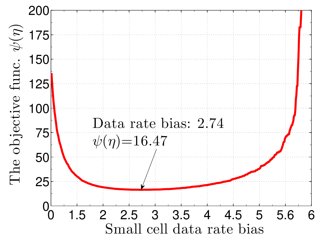
Fig. 6 shows the value of $\psi(\boldsymbol{\eta})$ versus the small cell data rate biases under the DRB-NU scheme. The value of $\psi(\boldsymbol{\eta})$ is minimized when the small cell data rate bias equals to 2.74. Given the data rate bias, the network’s traffic delivery latency is 17.24 and the brown power consumption is 480.9 $w$. Under the NUA scheme with $\kappa=2$, the network’s traffic delivery latency and the brown power consumption are 15.74 and 383.35 $w$, respectively. Therefore, as compared with the DRB-NU scheme, the NUA scheme reduces the traffic delivery latency and the brown power consumption by 8.7% and 20.28%, respectively. The NUA scheme has achieved enhanced performance because it allows individual BSs to adapt their network utility advertisements while the DRB-NU scheme only allows to change the data rate bias for an entire tier rather rather than for individual BSs. Another drawback of the DRB-NU scheme is that it does not dynamically respond to the network utility changes. The small cell data rate bias is optimized based on the previous instead of current network conditions, e.g., traffic intensities, backhaul constraints, and green power availabilities.

In Figs. 7, 9, 8, and 10, we compare the performance of three traffic load balancing schemes with varying network conditions. The first scheme is the green power and BS latency aware traffic load balancing scheme realized by vGALA with $\kappa=4$ and $\theta=0.5$ [16]. The second one is the NUA scheme that is aware of all network utilities. The third one, referred to as NUA-NC (no cache), is the NUA without awareness of the cache hit ratio. This scheme is realized by the NUA scheme with $\alpha_{j}=0,\;\forall j\in\mathcal{B}$. Fig. 7 shows the performance of these traffic load balancing schemes versus different backhaul data rates. When the backhaul data rate is very low, e.g., less than 5 Mbps in the simulation, the value of $\psi(\boldsymbol{\eta})$ and the traffic delivery latency under vGALA is very large. This indicates that, without the awareness of backhaul data rates, the traffic load balancing under vGALA congests some BSs in the network. The brown power consumption under vGALA does not change versus the backhaul data rates because vGALA does not consider the traffic delivery latency in backhaul as a performance metric in determining the user association. As the backhaul data rates increase, the value of $\psi(\boldsymbol{\eta})$ under these schemes converges because the backhaul constraint is gradually mitigated. However, the NUA scheme achieves smaller traffic delivery latency as compared with the vGALA scheme because of the awareness of the traffic delivery latency in backhaul.

In the simulation, the value of $\psi(\boldsymbol{\eta})$ is minimized by the NUA scheme. However, the NUA-NC scheme achieves the minimal traffic delivery latency as shown in Fig. 7(c). This is because the NUA scheme aims to minimize the value of $\psi(\boldsymbol{\eta})$ and thus strikes a tradeoff between the traffic delivery latency and the brown power consumption. As a result, compared with the NUA-NC scheme, the NUA scheme consumes less brown power at the cost of an increase of the traffic delivery latency.

The BSs’ coverage areas under these schemes are shown in Fig. 8. The NUA-NC scheme is aware of the backhaul limitation and thus reduces the coverage area of the backhaul constrained SCBS, e.g., SCBS 8. However, owing to the unawareness of the cache hit ratio, the NUA-NC scheme overestimates the traffic load in backhaul and constrains the coverage area of SCBSs, e.g., SCBS 8. The NUA scheme, being aware of the cache hit ratio of individual BSs, accurately estimates the traffic load in the backhaul and thus derives optimal coverage areas for BSs, e.g., increasing the coverage area of SCBS 8, to minimize the value of $\psi(\boldsymbol{\eta})$.

As shown in Fig. 9, when the backhaul data rate of a SCBS changes, e.g., $R_{5}$ reduces from 5 $Mbps$ to 1 $Mbps$, the NUA and NUA-NC scheme are able to adapt the traffic load balancing according to the backhaul data rate changes. However, the vGALA scheme, without the awareness of backhaul data rate, incurs excessive traffic delivery latency which is 667% of the traffic delivery latency of the NUA scheme as shown in Fig.9(c). As shown in Fig. 10, both the NUA and NUA-NC schemes are able to reduce the coverage area of SCBS 5. The NUA-NC scheme, because of the unawareness of the cache hit ratio, shrinks the coverage area more than the NUA scheme does.

Fig. 11 shows the the impact of the cache awareness on the traffic delivery latency. In the simulation, we set $\kappa=0$ for both the NUA scheme and the NUA-NC scheme to focus on the performance of the traffic delivery latency. Thus, both schemes are unaware of the green power utilization. As shown in Fig. Fig. 11, when the backhaul data rate is small, the cache awareness helps to reduce the traffic delivery latency.

References

- [1] T. Han, N. Ansari, M. Wu, and H. Yu, “On accelerating content delivery in mobile networks,” Communications Surveys Tutorials, IEEE, vol. 15, no. 3, pp. 1314–1333, Third 2013.
- [2] J. Andrews, S. Singh, Q. Ye, X. Lin, and H. Dhillon, “An overview of load balancing in HetNets: old myths and open problems,” Wireless Communications, IEEE, vol. 21, no. 2, pp. 18–25, April 2014.
- [3] T. Nakamura, S. Nagata, A. Benjebbour, Y. Kishiyama, H. Tang, X. Shen, N. Yang, and N. Li, “Trends in small cell enhancements in lte advanced,” Communications Magazine, IEEE, vol. 51, no. 2, pp. 98–105, February 2013.
- [4] H.-S. Jo, Y. J. Sang, P. Xia, and J. Andrews, “Heterogeneous cellular networks with flexible cell association: A comprehensive downlink SINR analysis,” IEEE Transactions on Wireless Communications, vol. 11, no. 10, pp. 3484–3495, Oct. 2012.
- [5] Q. Ye, B. Rong, Y. Chen, M. Al-Shalash, C. Caramanis, and J. Andrews, “User association for load balancing in heterogeneous cellular networks,” Wireless Communications, IEEE Transactions on, vol. 12, no. 6, pp. 2706–2716, June 2013.
- [6] H. Kim, G. de Veciana, X. Yang, and M. Venkatachalam, “Distributed optimal user association and cell load balancing in wireless networks,” IEEE/ACM Transactions on Networking, vol. 20, no. 1, pp. 177–190, Feb. 2012.
- [7] E. Aryafar, A. Keshavarz-Haddad, M. Wang, and M. Chiang, “RAT selection games in HetNets,” in INFOCOM, 2013 Proceedings IEEE, April 2013, pp. 998–1006.
- [8] X. Wang, M. Chen, T. Taleb, A. Ksentini, and V. Leung, “Cache in the air: exploiting content caching and delivery techniques for 5G systems,” Communications Magazine, IEEE, vol. 52, no. 2, pp. 131–139, February 2014.
- [9] K. Poularakis, G. Iosifidis, and L. Tassiulas, “Approximation algorithms for mobile data caching in small cell networks,” Communications, IEEE Transactions on, vol. PP, no. 99, pp. 1–1, Aug. 2014.
- [10] K. Shanmugam, N. Golrezaei, A. Dimakis, A. Molisch, and G. Caire, “Femtocaching: Wireless content delivery through distributed caching helpers,” Information Theory, IEEE Transactions on, vol. 59, no. 12, pp. 8402–8413, Dec 2013.
- [11] J. Monserrat, H. Droste, O. Bulakci, J. Eichinger, O. Queseth, M. Stamatelatos, H. Tullberg, V. Venkatkumar, G. Zimmermann, U. Dotsch, and A. Osseiran, “Rethinking the mobile and wireless network architecture: The METIS research into 5G,” in Networks and Communications (EuCNC), 2014 European Conference on, June 2014, pp. 1–5.
- [12] T. Han and N. Ansari, “On greening cellular networks via multicell cooperation,” IEEE Wireless Communications Magazine, vol. 20, no. 1, pp. 82–89, 2013.
- [13] Z. Hasan, H. Boostanimehr, and V. Bhargava, “Green cellular networks: A survey, some research issues and challenges,” IEEE Communications Surveys and Tutorials, vol. 13, no. 4, pp. 524–540, 2011.
- [14] T. Han and N. Ansari, “Powering mobile networks with green energy,” Wireless Communications, IEEE, vol. 21, no. 1, pp. 90–96, February 2014.
- [15] Ericson Inc., “Sustainable energy use in mobile communications,” Aug. 2007, white Paper.
- [16] T. Han and N. Ansari, “A traffic load balancing framework for software-defined radio access networks powered by hybrid energy sources,” CoRR, vol. abs/1407.7780, 2014. [Online]. Available: http://arxiv.org/abs/1407.7780
- [17] ——, “On optimizing green energy utilization for cellular networks with hybrid energy supplies,” IEEE Transactions on Wireless Communications, vol. 12, no. 8, pp. 3872–3882, Aug. 2013.
- [18] L. Wang and G.-S. Kuo, “Mathematical modeling for network selection in heterogeneous wireless networks: A tutorial,” Communications Surveys Tutorials, IEEE, vol. 15, no. 1, pp. 271–292, First 2013.
- [19] A. Damnjanovic, J. Montojo, Y. Wei, T. Ji, T. Luo, M. Vajapeyam, T. Yoo, O. Song, and D. Malladi, “A survey on 3GPP heterogeneous networks,” Wireless Communications, IEEE, vol. 18, no. 3, pp. 10–21, June 2011.
- [20] S. Singh, H. Dhillon, and J. Andrews, “Offloading in heterogeneous networks: Modeling, analysis, and design insights,” Wireless Communications, IEEE Transactions on, vol. 12, no. 5, pp. 2484–2497, May 2013.
- [21] F. Pantisano, M. Bennis, W. Saad, and M. Debbah, “Cache-aware user association in backhaul-constrained small cell networks,” in the 12th International Symposium on Modeling and Optimization in Mobile, Ad Hoc, and Wireless Networks (WiOpt 2014), May 2014, pp. 37–42.
- [22] J. Zhou, M. Li, L. Liu, X. She, and L. Chen, “Energy source aware target cell selection and coverage optimization for power saving in cellular networks,” in Proceedings of the 2010 IEEE/ACM Int’l Conference on Green Computing and Communications, Hangzhou, China, Dec. 2010.
- [23] T. Han and N. Ansari, “Green-energy aware and latency aware user associations in heterogeneous cellular networks,” in Proceedings of IEEE Global Telecommunications Conference (GLOBECOM’13), Atlanta, GA, USA, Dec 2013, pp. 4946–4951.
- [24] H. Gomaa, G. Messier, C. Williamson, and R. Davies, “Estimating instantaneous cache hit ratio using markov chain analysis,” Networking, IEEE/ACM Transactions on, vol. 21, no. 5, pp. 1472–1483, Oct 2013.
- [25] L. Breslau, P. Cao, L. Fan, G. Phillips, and S. Shenker, “Web caching and Zipf-like distributions: evidence and implications,” in the Eighteenth Annual Joint Conference of the IEEE Computer and Communications Societies., vol. 1, Mar 1999, pp. 126–134 vol.1.
- [26] P. Rodriguez, C. Spanner, and E. W. Biersack, “Analysis of web caching architectures: Hierarchical and distributed caching,” IEEE/ACM Transactions on Networking, vol. 9, no. 4, pp. 404–418, Aug. 2001.
- [27] P. Jelenkovic and A. Radovanovic, “Asymptotic insensitivity of least-recently-used caching to statistical dependency,” in the Twenty-Second Annual Joint Conference of the IEEE Computer and Communications., vol. 1, March 2003, pp. 438–447 vol.1.
- [28] Y. Zhang, N. Ansari, M. Wu, and H. Yu, “On wide area network optimization,” Communications Surveys Tutorials, IEEE, vol. 14, no. 4, pp. 1090–1113, Fourth 2012.
- [29] L. Kleinrock, Queueing Systems: Computer applications. Wiley-Interscience, 1976, ISBN: 978-0471491118.
- [30] A. Farbod and T. D. Todd, “Resource Allocation and Outage Control for Solar-Powered WLAN Mesh Networks,” IEEE Transactions on Mobile Computing, vol. 6, no. 8, pp. 960–970, Aug. 2007.
- [31] G. Auer, V. Giannini, C. Desset, I. Godor, P. Skillermark, M. Olsson, M. Imran, D. Sabella, M. Gonzalez, O. Blume, and A. Fehske, “How much energy is needed to run a wireless network?” Wireless Communications, IEEE, vol. 18, no. 5, pp. 40 –49, Otc. 2011.
- [32] “Evolution of land mobile radio (including personal) ccommunications: COST 231.” [Online]. Available: http://www.awe-communications.com/Propagation/Urban/COST/
- [33] “HIT photovoltaic module.” [Online]. Available: http://us.sanyo.com/dynamic/product/Downloads/Panasonic%20HIT%20220A%20Data%20Sheet_WEB-10609680.pdf
- [34] C. Riordan and R. Hulstron, “What is an air mass 1.5 spectrum? [solar cell performance calculations],” in Photovoltaic Specialists Conference, 1990., Conference Record of the Twenty First IEEE, May 1990, pp. 1085–1088.