Efimov-like phase of a three-stranded DNA and the renormalization-group limit cycle

Tanmoy Pal Affiliation: Institute of Physics, Bhubaneswar 751005 India email: tanmoyp@iopb.res.in Poulomi Sadhukhan Affiliation: Institute of Physics, Bhubaneswar 751005 India Affiliation: Present address: Institut für Theoretische Physik, Universität Göttingen, Friedrich-Hund-Platz 1, 37077 Göttingen, Germany Somendra M. Bhattacharjee Affiliation: Department of Physics, Ramakrishna Mission Vivekananda University, Belur Math, West Bengal 711202, India email: somen@iopb.res.in; somen@rkmvu.ac.in Affiliation: Institute of Physics, Bhubaneswar 751005 India

Abstract

A three-stranded DNA with short range base pairings only is known to exhibit a classical analog of the quantum Efimov effect, viz., a three-chain bound state at the two chain melting point where no two are bound. By using a non-perturbative renormalization-group method for a rigid duplex DNA and a flexible third strand, with base pairings and strand exchange, we show that the Efimov-DNA is associated with a limit cycle type behavior of the flow of an effective three-chain interaction. The analysis also shows that thermally generated bubbles play an essential role in producing the effect. A toy model for the flow equations shows the limit cycle in an extended three-dimensional parameter space of the two-chain coupling and a complex three-chain interaction.

I Introduction

As the storehouse of the genetic code, DNA is one of the most important molecules in biology [1]. Structurally it is a polymer made of bases, normally of four kinds, A, T, G, and C, whose sequence along the chain codes for the amino acids of proteins. DNA is generally found in a double helical (dsDNA) form with two strands attached to each other by the classic Watson-Crick type of hydrogen bonding of A with T, and G with C; still many other alternative conformations are known [2]. One such example is the triplex or triple stranded DNA which can also be of several types. In one form, for special sequences, the third strand binds to a dsDNA via the Hoogsteen base pairing and forms a triple helix structure [3, 4, 5]. In another case, one dsDNA locally melts forming a bubble and one strand of the bubble may pair with a third strand, provided it has a sequence of matching complementary bases. This is called strand exchange [6]. It was argued in Refs. [7, 8, 9, 10] that near the thermal melting of a dsDNA, the formation of large bubbles enhances the possibility of a strand exchange involving each strand of the bubble. This leads to an effective long range attraction of the original pair, mediated by the third strand. As a result, a three-strand bound state is formed where no two are bound. Such a novel state of DNA, produced by fluctuations, has been called an Efimov-DNA in analogy with the Efimov effect in three-body quantum mechanics [11, 12, 13, 14, 15].

DNA is nothing but two polymers, each one made of monomers (bases) connected linearly, and with interaction between two monomers of the two polymers only if they have the same contour length measured from one physical end. This interaction is called the native DNA interaction, and it produces the bound dsDNA. Thermal fluctuations can break hydrogen bonds locally, making bubbles in the bound state. When all the base pairs are broken, either by thermal fluctuations or by a force, releasing the two chains, one gets a melting or an unzipping transition of DNA [16, 17, 18, 19]. These transitions are of importance in biology for their inherent functional utility, and in polymer physics, as examples of “few-chain” problems involving the interplay of polymer correlations and mutual interactions (as opposed to polymer solutions [20]). To this list of few-chain problems, is now added the fluctuation-driven Efimov-DNA.

The Efimov effect was studied originally as a three-body quantum mechanics problem by solving the Schrödinger equation in the Fadeev approach [11, 12, 13, 14, 15]. Several approximate methods were also used, most notable among which is the use of the Born-Oppenheimer approximation for a separable short range potential [21]. Such calculations show the emergence of the scale-free $1/r^{2}$ attraction at the quantum critical point of unbinding, as does the polymer scaling of Ref. [7]. Field theoretic methods were initiated much later on as an effective field theory for few-body quantum mechanics. Some successes were met in the diatom approach where the effect was studied in the scattering of a single particle from a diatom [15, 22]. The major effort in these attempts was to see the Efimov effect as a universal effect, emerging from a diverging length scale, here the scattering length. It led to the idea of a limit cycle renormalization group (RG) flow [23], which was introduced in a different context in Ref. [24]. The characteristic signature of the effect is the geometric sequence ( $E_{n}=a^{n}E_{0}$ ) of energy eigenvalues, the Efimov tower, and it is believed to emanate from this limit cycle behaviour. It occurs only at the point where the length scale diverges. For nearby points one still gets three-body bound states but with a finite number of states. Although proposed in nuclear physics, experimental signatures for the Efimov effect started pouring in only after the technological developments in handling cold atoms [25, 26, 27].

The possibility of an Efimov-DNA was first pointed out by using a scaling argument and by a real space renormalization group approach to three polymers that can be implemented exactly for hierarchical lattices [7, 8]. That the melting transition with a large or diverging length scale is crucial (equivalent to infinite scattering length in the quantum version) was clearly brought out by the polymer scaling, that reproduces the $1/r^{2}$ interaction, where $r$ is the distance between two polymers. This interaction owes its origin to the long range polymer correlations in a big bubble. The importance of the transition was also made clear in studies of the DNA problem in lower dimensional fractal lattices. In fact, a mixed phase different from the Efimov dna was predicted, for which a quantum analog is not known [9]. On the polymer front, the strangeness of the long-range interaction is evident from the renormalization-group analysis of two polymers with $-g/r^{2}$ interaction in the presence of a short range attraction [28, 29, 30]. The unbinding transition is described, as usual, by a fixed point, but that is not all. First, the fixed point is $g$ -dependent, and, second, the order of the transition is determined by the reunion exponent of the bubbles at the $g$ -dependent fixed point describing the unbound phase [31]. More unusual is the possibility of complex fixed points. This happens for $g>1/4$ . The complex fixed points are responsible for certain periodicity of various thermodynamic quantities and is similar to the origin of the Efimov tower. A direct proof of the long range interaction is still not possible but the emergence of a limit cycle behaviour in Euclidean three dimensions was reported in Ref. [10].

The similarity between the zero temperature quantum problem and the classical thermal system of polymers actually follows from an imaginary time transformation of the quantum problem in the path integral approach [7]. For example, a path integral computation of the quantum problem could identify polymer like phases [32]. The fluctuations in the size of the polymer bubbles near the melting point of dsDNA play a similar role as that of quantum fluctuations near the unbinding transition of a pair of particles. The DNA bubbles correspond to the paths in the classically forbidden region of the short range potential [33]. In this paper, we elaborate on the link between the Efimov-DNA and a limit cycle behaviour in a renormalization group approach. Our results show that there are many other similarities of the results for a DNA with the diatom trick used in the quantum version and it reinforces the idea that the features of the quantum Efimov effect could be observed in a classical setting of DNA in a solution.

The idea of RG is to look at a problem based on length scales and not on the numerical values of the parameters per se. How the various parameters change with the length scale then tells us the behaviour of the macroscopic system in the large size limit. The procedure is to (i) integrate out the small length scale fluctuations, especially bubbles and (ii) then by rescaling generate a similar system but with renormalized parameters. The flows of the parameters as the scale is changed give us all the crucial large length-scale results. The interpretation of the RG flows adopted here, discussed in detail below, is different from the one generally done for polymers [34, 28, 29] but similar in spirit as done in quantum field theories, especially in the context of the Efimov effect [15]. In general, an RG approach is expected to lead to fixed points and separatrices, at most lines of fixed points. The fixed points represent states of the system which show scale invariance under a continuous rescaling of lengths. As pointed out above, it is rather rare to see a limit-cycle-like behaviour because its periodicity would produce a discrete scale invariance only.

Refer to caption — Figure 1: (Color online) Schematic diagram of a strand exchange and the equivalent coarse-grained three-chain interaction $g_{3}$ . (a) A single strand [blue line marked (1)] pairs with one strand of a bubble on a duplex [brown lines marked (2)]. The short vertical (green) lines indicate base pairings, with the energy per unit length $\epsilon$ . The junction weight $g_{2}$ is associated with each fork or the interface on a duplex. In (a) there are four interfaces as indicated by the arrows. (b) A coarse-grained version of (a) where the duplex is represented by a thick line interacting with the single line. The filled circle represents the three-chain interaction $g_{3}$ .

Polymer problems traditionally start with a random walk or a Gaussian polymer as the primary representation of a polymer. Most of the DNA melting theories are of this type where the free model represents the unbound states. In the Gaussian polymer model (no self-interaction), the melting transition is continuous [35, 36] so that the closer one is to the melting temperature, the larger is the size of the thermally generated bubbles. In this approach the two-chain and the three-chain problems have critical dimensionality $d=2$ and $d=1$ respectively [34]. Evidently a strand exchange for a small bubble in a three-chain system would, on scales larger than the bubble size, look like a three-strand interaction (Fig. 1). Therefore, in three dimensions, one needs to consider irrelevant variables and, so, a straightforward perturbative RG fails here. This makes a complete analysis of the three-chain problem formidable. To circumvent this, a different approach is adopted here. Instead of flexible Gaussian or semiflexible polymer representations, we model the dsDNA as a sequence of rigid rod like bound segments and bubbles made of flexible Gaussian chains at finite temperature. Thus the melting point is approached from the bound state side via the formation of bubbles. We allow strand exchange in the bubble region of a pair and study the behaviour of the three-body interaction generated as the short distance cutoff is taken to zero. In the Fourier space, the limit corresponds to the upper cutoff $\Lambda\to\infty$ . The resulting RG flow equation shows a limit cycle behaviour, due to critical fluctuations, via nonphysical complex fixed points. Unlike the cases with special long range forces, here all the interactions are strictly short ranged (like hydrogen bonds for DNA).

The effect of fluctuations is not just restricted to the melting point itself. Even above the melting point, the bound state persists, eventually melting at a temperature higher than the duplex melting temperature. The limit cycle that occurs at the melting point is actually unstable as we move away from this special point. The number of turns in a way determines the number of bound states. Beyond a certain point all such states vanish. This point or temperature will be the melting point of the Efimov DNA.

The outline of the paper is given below. The model is defined in Sec. II.1 in real space. It involves the bound state of dsDNA as a rigid chain and the third strand as a flexible chain. The interfacial term that helps in bubble formation through forking, and the three chain interaction are defined here too. A brief overview of what is expected in a limit cycle RG is given in Sec. II.2. The calculations are done in the Fourier-Laplace space. The necessary rules for diagrams and the form of the partition functions are given in Sec. II.3. We approach from the bound to the unbound side. For the two-chain bound state at finite temperatures, forking is allowed with some energy cost. Two successive forkings result in the formation of a bubble which can be infinite in number. The corresponding duplex partition function and the melting of the rigid DNA are discussed in Sec. III. The three-chain case where we consider the duplex–free-chain interaction can be found in Sec. IV. Two cases are considered there. A case with no bubbles in the dsDNA is in Sec. IV.1 while the whole three-chain part is analyzed at the two body critical point in Sec. IV.2. A few details can be found in the appendixes. In particular, Appendix C is about a toy example that extrapolates between the flow equations for the three chain interaction with no bubbles and the same at the critical melting point. We end with a discussion of the results and their experimental consequences in Sec. V and a short summary in Sec. VI.

II Model and result

II.1 Model

Our model of three polymer chains is defined, à la Poland-Scheraga, through their partition functions. Every monomer lives in a $d$ -dimensional space. All chains are of equal length $N$ . They are tied at one end at origin in space while the other end may also be tied together at a point ${\bf r}$ , though the latter constraint may be relaxed. One end needs to be kept together to prevent any chain from flying away, thereby facilitating the bookkeeping for entropy. The monomers on different chains interact only when they are at the same space ( $\bf r$ ) and length ( $z$ ) coordinates. Such an attractive interaction corresponds to the native base pairing of DNA.

The basic constituents of the model are the partition functions for a single chain, for a bound pair, the weight $g_{2}$ for dissociation of a pair or joining of two chains (Y forks), and the interaction $g_{3}$ between a single chain and a bound pair. The two important parameters in this problem are $g_{2}$ and $g_{3}$ .

We first define the basic partition functions, viz., (i) ${\sf Z}({\bf r},N)$ for a single chain, and (ii) ${\sf Z}_{b}({\bf r},N)$ for a pure bound state of two strands.

II.1.1 Single chain

A single strand is a flexible Gaussian chain with

{\sf Z}({\bf r},N)={\mu^{N\Lambda^{2}}}\ \frac{1}{(2\pi N)^{d/2}}\ e^{-\frac{{\bf r^{2}}}{2N}},

(1)

where $\mu^{N\Lambda^{2}}$ is the total number of configurations, and $\Lambda^{-1}$ is a short distance or microscopic cutoff. For a Gaussian chain the overall size $R$ of a polymer scales as

R^{2}\sim N,

(2)

which allows us to set the dimension of $N$ as

[N]={\rm L}^{2},\quad{\rm when\ }[r]=[\Lambda^{-1}]={\rm L},

(3)

the square bracket $[...]$ indicating the dimensionality of the enclosed entity. In Eq. (1), $\Lambda$ is used to make $N$ dimensionless in the $\mu$ -dependent factor. The unconstrained entropy of a free chain is taken as $\propto\ln\mu$ per unit length to avoid the problem of an infinite entropy of a continuous chain. The Gaussian factor in Eq. (1) is the probability density of finding the end of the polymer at ${\bf r}$ , so that the total partition function after integration over all space is dimensionless.

II.1.2 Bound state, Y fork, duplex, and $g_{2}$

The second partition function needed is for the two-chain bound state which is taken as a rigid rod with $\epsilon\Lambda^{2}$ as the binding energy per unit length. The bound DNA with one end fixed can rotate in space as a whole but can not bend. The partition function of the bound state of length $N$ is given by

{\sf Z}_{\sf b}({\bf r},N)=\frac{1}{4\pi}\;e^{-\epsilon N\Lambda^{2}}\;\delta({\bf r}-N\Lambda\hat{\bf n}),

(4)

where $\hat{\bf n}$ is a unit vector giving the direction of the rigid rod.

Now, there are finite temperature fluctuations in the form of pair breaking. The bound state then locally dissociates into two single strands to form a Y fork. The two free strands may rejoin to produce a bubble. We assign an interface weight $g_{2}$ in the partition function for every Y fork. This is like an extra interfacial contribution and is referred to as the “co-operativity factor” [9]. It is shown below Eq. (20), that dimensionwise


$\displaystyle[g_{2}^{2}]$	$\displaystyle=$	$\displaystyle[\Lambda]^{4-d},$	(5a)
	$\displaystyle=$	$\displaystyle[\Lambda]^{1},\quad(d=3).$	(5b)

The importance of bubbles is well-recognized both in the biological functions and in physical properties of DNA. There have been many studies, in recent times, both theoretical and experimental, on the nature and functions of the bubbles under various situations, like DNA under a force or topological constraints [37, 38, 39, 40, 41], in breathing dynamics [42, 43, 44, 45], in hysteresis [46, 47], with semiflexibility [48], etc.

The introduction of finite temperature bubbles makes the bound state flexible and as a result it can bend. We name this bound state with bubbles a duplex. The $g_{2}$ -dependent partition function ${\sf Z}_{\sf d}$ is discussed in Sec III. We see there that the formation of large bubbles, by thermal fluctuations leads to the melting of a duplex into two free chains, at a critical value of $g_{2}=g_{2c}$ . The role of $g_{2}$ may be represented by the sequence of partition functions

\underbrace{\sf Z_{b}}_{\{g_{2}=0\}}\stackrel{{\scriptstyle{\rm crossover}}}{{\longrightarrow}}\underbrace{\sf Z_{d}}_{\{g_{2}<g_{2c}\}}\stackrel{{\scriptstyle{\rm melting}}}{{\longrightarrow}}\underbrace{\sf Z^{2}}_{\{g_{2}>g_{2c}\}},

(6)

where the change from a rigid to an elastic one by $g_{2}$ is a crossover (not a transition).

II.1.3 Strand exchange and $g_{3}$

For the three-polymer system, we consider the situation where a pair is in the bound or duplex state and the other one is free. The third chain is allowed to interact with a free strand of a bubble allowing it to form a duplex locally. This is called strand exchange. Figure 1 illustrates this process schematically.

The pair interaction together with the strand exchange would, in principle, be sufficient to formulate the three-chain DNA problem, but in a renormalization group approach, the three-chain bound state is described by a three-chain interaction. Therefore, in anticipation of its generation, we allow a three-chain interaction (between a single chain and a duplex) $g_{3}$ . This interaction parameter is our three-body coupling. We see below Eq. (28) that it has the dimensionality


$\displaystyle[g_{3}]$	$\displaystyle=$	$\displaystyle[\Lambda]^{2-d},$	(7a)
	$\displaystyle=$	$\displaystyle[\Lambda]^{-1}\quad(d=3).$	(7b)

The dimensionless three-chain parameter may now be constructed as [49]

\displaystyle H(\Lambda)

\displaystyle=

\displaystyle-\;\frac{g_{3}}{4g_{2}^{2}}\Lambda^{2},

(8)

with a factor of $4$ for convenience.

The partition function for three chains depends on both $g_{2}$ and $g_{3}$ but for a duplex it depends only on $g_{2}$ .

II.2 Qualitative description

Our aim is to see the effect of strand exchange on the three-chain system near the duplex melting point where large sized bubbles are expected. Right at the melting point, we may concentrate on how $g_{3}$ or $H$ evolves as $\Lambda\to\infty$ for large $N$ . A flow of $H$ from zero to $+\infty$ is an indication of a three-chain bound state [note the negative sign in Eq. (8)], the Efimov-DNA case of a bound three-chain system where no two are bound.

In the RG approach the flows of parameters are obtained in a few steps. With a reciprocal space upper cutoff $\Lambda$ (a short distance scale $\sim\Lambda^{-1}$ ), the effects over a range $\Lambda$ to $\Lambda-d\Lambda$ are taken into account by redefining the problem for scales up to $\Lambda-d\Lambda$ . A subsequent rescaling brings back the problem to the original scale with renormalized parameters. The changes in the parameters, as continuous variables, gives us the flow equations or $\beta$ functions

\Lambda\frac{\partial H}{\partial\Lambda}=\beta(H).

(9)

The behaviour of a system is then characterized by the flows which generally terminate at stable fixed points (or at infinity) separated by unstable fixed points. The fixed points represent the phases and the phase transitions in the system. This is the generic picture of RG and this is where the three-chain problem stands out.

In our approach, $g_{2}$ is the control parameter for the duplex melting. We first determine the critical point of melting by locating the critical value $g_{2c}$ at which a suitably defined length scale $\xi$ diverges. At this particular point we determine the RG flow or the $\beta$ function for $H(\Lambda)$ . Quantitatively this is implemented by calculating the third virial coefficients, obtained from the connected three-chain partition function (i.e., for polymers connected by the interactions).

A naive use of the definition, Eq. (8), suggests the form

	$\beta(H)=2H,\quad({\rm{naive}}).$	(10a)
This however gets modified by the effects of strand exchange and other fluctuations to a form
	$\beta(H)=2H+{\cal F}(H),\quad({\rm with\ renormalization}),$	(10b)

and all the nontriviality comes from these additional terms. In general, it has a form

\beta(H)=-AH^{2}+BH+C,

(11)

$A,B,C$ being all real. In conventional cases, $B$ is mainly determined by the naive dimensional analysis, while a nonzero $A$ is the extra addition of length rescaling and renormalization. A constant term $C$ is unusual and appears if there are marginal parameters, which do not change with length scales. An example of a marginal parameter is $g$ of the inverse square interaction mentioned in the Introduction. This identification may be turned around to argue that a constant term in the $\beta$ function signals the presence of some, may be hidden, marginal parameter in the problem.

If $C$ in Eq. (11) is such that there are two real roots of $\beta(H)=0$ , the standard picture remains valid with one stable and one unstable fixed points, but not so if the roots are complex conjugate pairs [for $C<-B^{2}/(4A)$ ]. Such is the case for the problem in hand. We find

\Lambda\frac{\partial H}{\partial\Lambda}=-A(H-H_{0})(H-H_{0}^{*}),

(12)

where $H_{0},H_{0}^{*}$ form a complex-conjugate pair.

The procedure we adopt to derive Eq. (12) is different from the conventional RG way. The traditional approach is to take into account the effects at the short distance level to redefine the parameters on a larger length scale. Instead of such an approach we determine the effective parameter as an integral equation and then use a thin-shell integration method to get the $\Lambda$ dependence of $H$ by demanding the existence of a cutoff independent limit. From this we reconstruct the $\beta$ function. Then we argue that at the duplex melting point the $\beta$ function of the dimensionless scaled three-body interaction parameter $H$ has the same form as that of Eq. (12) and the limit cycle describes the three-body bound Efimov states.

The nonconformity with the standard picture of fixed points has a far reaching consequence of converting the continuous scaling symmetry at the unstable fixed point to a discrete symmetry. The continuous scaling symmetry at a real fixed point leads to power law behaviours of physical quantities. Contrary to that, complex fixed points invoke a limit-cycle-type behaviour in the RG flow trajectories. An outcome of the generated periodicity is a discrete scaling symmetry and the relevant parameter, here $H$ , repeats itself in a log periodic manner. In the quantum language, this discrete symmetry leads to the Efimov tower of the energies.

II.3 Diagrammatic definitions and rules

Since we shall be using diagrammatic representations for many equations, it is prudent to define our model in terms of diagrams and the rules for computations. To take advantage of the convolution property of the Fourier and the Laplace transforms, we work in the Fourier-Laplace space $({\bf k},s)$ instead of $({\bf r},N)$ . The conventions for these transforms are

	$\displaystyle{\hat{Z}}({\bf k},N)$	$\displaystyle=$	$\displaystyle\int{\sf Z}({\bf r},N)e^{-i{\bf k.r}}\;d^{d}r,$		(13)
	$\displaystyle Z({\bf k},s)$	$\displaystyle=$	$\displaystyle\int_{0}^{\infty}{\hat{Z}}({\bf k},N)e^{-Ns}dN,$		(14)

with the inverse transforms defined as

	$\displaystyle{\sf Z}({\bf r},N)=\frac{1}{(2\pi)^{d}}\int{\hat{Z}}({\bf k},N)e^{i{\bf k.r}}d^{d}k,$		(15)
	$\displaystyle Z({\bf k},N)=\frac{1}{2\pi i}\oint Z({\bf k},s)e^{Ns}ds.$		(16)

The contour for the integration in Eq. (16) is the usual Mellin’s contour.

The dimensionalities of the partition functions, as per our conventions, are as follows


	$\displaystyle[{\sf Z}({\bf r},N)]={\rm L}^{-d},[{\hat{Z}}({\bf k},N)]={\rm L}^{0},$		(17a)
	$\displaystyle[Z({\bf k},s)]={\rm L}^{2},{\rm\ with\ }[s]={\rm L}^{-2}.$		(17b)

These $L$ dependencies are used to identify the dimensionalities of the remaining parameters.

II.3.1 Free chain

In the Fourier-Laplace space the single chain partition function, Eq. (1), becomes

Z({\bf k},s)=\frac{1}{s-\Lambda^{2}\ln\mu+\frac{k^{2}}{2}}.

(18)

To be noted here is that the free energy per unit length comes from the pole of Eq. (18) in the complex- $s$ plane. This partition function, Eq. (18), to be called a propagator, is represented by a solid line in Fig. 2(a).

II.3.2 Bound state

The rigid bound state of Eq. (4) is direction dependent. For simplicity we take an average over all directions by integrating over the solid angle subtended by $\hat{\bf n}$ (see Appendix A). The corresponding Fourier-Laplace transformed partition function is given by

Z_{\sf b}({\bf k},s)=\frac{1}{k\Lambda}\arctan\frac{k\Lambda}{s+\epsilon\Lambda^{2}}\stackrel{{\scriptstyle k\rightarrow 0}}{{=}}\frac{1}{s+\epsilon\Lambda^{2}}.

(19)

The $k\rightarrow 0$ form of $Z_{\sf b}({\bf k},s)$ can be used close to the melting defined shortly. Here also the pole in the complex $s$ plane gives the free energy of the rigid bound state. The bound-state partition function of Eq. (19) is represented by an unfilled rectangular box in Fig. 2(b).

At finite temperatures, the inclusion of the Y forks gives the duplex partition function $Z_{\sf d}({\bf k},s)$ represented by a filled black box in Fig. 3(a).

The Y-fork junction, $g_{2}$ , is represented in Fig. 2(c) by a vertex where a rectangular box (a bound pair) and two solid lines (free chains) meet. The diagram in Fig. 3(c) represents an interaction between a duplex and a free chain. The interaction is the three-body coupling constant given by $g_{3}$ .

II.4 ${\bf k}$ and $s$ Conservation

As all the partition functions have translation invariance we have ${\bf k}$ conservation at each vertex. Following the standard nomenclature, the ${\bf k}$ vectors are called “momentum.” So momentum is conserved at each vertex. Also cutoff $\Lambda$ is called a momentum cutoff.

The Y fork and the three-chain interaction can take place anywhere along the length of the polymers which are infinitely long. This invariance (translational invariance along the contour) leads to an $s$ -conservation at any point. In other words, at a junction $s$ -values get distributed, but the total remains the same. More details are discussed in Appendix B.

III Two Chains

At first let us find the duplex partition function. In the grand canonical ensemble (Laplace space) the singularity of the partition function closest to the origin gives the free energy of the system; contributions from others are suppressed in the thermodynamic limit. Whenever there is a switching of the nearest singularity due to a change in some parameter of the system, we have a phase transition. Henceforth all the calculations are done in $d=3$ .

Considering an arbitrary number of bubbles we can write the finite temperature bound state as a sum of an infinite number of diagrams shown in Fig. 3(a). In terms of the Laplace variable $s$ , the duplex partition function, denoted by $Z_{\sf d}({\bf k},s),$ can be written as a geometric series

	$\displaystyle Z_{\sf d}({\bf k},s)$	$\displaystyle=$	$\displaystyle Z_{\sf b}({\bf{k}},s)+g_{2}^{2}\;Z_{\sf b}({\bf{k}},s)\;I_{0}\;Z_{\sf b}({\bf{k}},s)+....$		(20)
		$\displaystyle=$	$\displaystyle\frac{1}{\frac{1}{Z_{\sf b}({\bf{k}},s)}-g_{2}^{2}I_{0}},$		(20)

where $I_{0}$ , the single bubble contribution, is given by

	$\displaystyle I_{0}$	$\displaystyle=$	$\displaystyle\int\frac{d{\bf q}}{(2\pi)^{3}}\;\frac{d\bar{s}}{2\pi i}\;Z\left(\frac{{\bf k}}{2}-{\bf q},\bar{s}\right)\;Z\left(\frac{{\bf k}}{2}+{\bf q},s-\bar{s}\right)$		(21)
		$\displaystyle=$	$\displaystyle\frac{1}{2\pi^{2}}\left[\Lambda-\sqrt{s^{\prime}+k^{2}/4}\;\arctan\frac{\Lambda}{\sqrt{s^{\prime}+k^{2}/4}}\right],$		(21)

and $s^{\prime}=s-2\Lambda^{2}\ln\mu$ . Equation (20), with Eqs. (17a) and (17b), sets the dimension of $g_{2}$ as quoted in Eq. (5a).

To evaluate $I_{0}$ we do the $\bar{s}$ integral by the method of residues. See Appendix B for details. The only contribution comes from the simple pole at $\bar{s}=\Lambda^{2}\ln\mu-({\bf k}/2-{\bf q})^{2}/2$ . In the limit $(s^{\prime}+k^{2}/4)\rightarrow 0$ and $\Lambda$ finite, which is the relevant limit near the transition point, we have

I_{0}=\frac{1}{2\pi^{2}}\left[\Lambda-\frac{\pi}{2}\sqrt{s^{\prime}+k^{2}/4}\right].

(22)

So the duplex partition function becomes

Z_{d}({\bf k},s)=\left\{s+\epsilon\Lambda^{2}-\frac{1}{2\pi^{2}}g_{2}^{2}\left[\Lambda-\frac{\pi}{2}\sqrt{s^{\prime}+k^{2}/4}\right]\right\}^{-1}.

(23)

We identify here three different singularities in the partition function $Z_{\sf d}$ , which correspond to three distinct states. The branch point singularity of Eq. (23) at $s=2\Lambda^{2}\ln\mu$ , owing its origin to $Z$ , gives the completely unbound (denatured) state. This is the high temperature phase. The singularity at $s=-\epsilon\Lambda^{2}$ corresponds to the completely bound state when $g_{2}=0$ . This, being the singularity of $Z_{\sf b}$ , is the zero temperature phase and does not survive when $g_{2}\neq 0$ . The third singularity $s^{\prime}_{*}$ comes from the zero of the denominator of $Z_{\sf d}(0,s)$ . As $s^{\prime}_{*}$ continuously evolves with $g_{2}$ from $s=-\epsilon\Lambda^{2}$ , it corresponds to a bound state with bubbles. In the absence of $g_{2}$ , i.e., in absence of any interface or junction point, there can be two states only; the system stays either in the completely bound state or in the completely unbound state. There could be a denaturation transition, necessarily first order, by changing $\epsilon$ or $\mu$ . This case is of no interest to us. The presence of the interface alters the nature of the bound state because of the bubbles and also makes the transition critical [see Eq. 6].

Our main aim is to concentrate on the behaviour of the system near duplex melting where the contributions from the bubbles (loops) of large sizes dominate the duplex partition function. In the small $s^{\prime}$ limit with $k=0$ , $s^{\prime}_{*}$ is given by

\sqrt{s^{\prime}_{*}}=-\frac{\Delta t}{2\pi^{2}g_{2}^{2}\Lambda^{-2}},

(24)

where $\Delta t\equiv(2\pi)^{3}(2\ln\mu+\epsilon)-4\pi g_{2}^{2}\Lambda^{-1}$ . $s^{\prime}_{*}$ can be identified as the difference of free energies between duplex and two free chain states. So, $\Delta t$ is a measure of deviation from the duplex melting point. The equation $\Delta t=0$ [50] gives the critical point as

g_{2c}=\sqrt{2\pi^{2}(2\ln\mu+\epsilon)\Lambda}.

(25)

The thermal melting of a dsDNA can also be illustrated from this model [51]. Using Eq. (24), we define a diverging length scale $\xi$ in the following way

s^{\prime}_{*}\sim\xi^{-2},\ {\rm with}\ \xi\sim|\Delta t|^{-1}.

(26)

If we now make a scale change such that, for arbitrary $b$ , ${\bf k}\rightarrow b^{-1}{\bf k}$ , the length scale changes as $\xi\rightarrow b\xi$ . And as $s^{\prime}_{*}$ is the free energy difference, the free energy scales as $f\rightarrow b^{-2}f$ . This is the continuous scale invariance satisfied at the thermal dsDNA melting.

By tuning $g_{2}$ the length scale $\xi$ can be made divergent for some critical value of $g_{2}$ , $g_{2c}$ . Beyond it, the system goes to a stable high temperature phase with two free chains. The full duplex partition function can be written for small $s^{\prime}$ as

Z_{\sf d}({\bf k},s)=\frac{(2\pi)^{3}}{{2\pi^{2}g_{2}^{2}\left[-{\xi}^{-1}+\sqrt{s^{\prime}+k^{2}/4}\right]}},

(27)

which explicitly shows the $\xi$ dependence.

IV Three Chains

Now consider the three-chain problem. The effect of thermal fluctuations (bubbles) are very important in our model. To make this more clear, we first consider the case where the bubbles are not allowed. Next, we consider the case with bubbles.

IV.1 No bubbles: $g_{2}=0$

Let us first consider the case of a free chain interacting with a bound state. Here we set $g_{2}=0$ such that there are no bubbles in the bound state. This problem with interaction up to all orders can be solved by solving the diagrammatic integral equation shown in Fig. 4 (see Appendix B).

The bare single chain bound state contact interaction is $g_{3}$ and we denote the corresponding renormalized interaction by $V$ . Evaluations of Fig. 4 in $d-$ dimensions give us

V=-g_{3}-g_{3}V\int\frac{d{\bf q}}{(2\pi)^{d}}\;\frac{d\bar{s}}{2\pi i}\;Z({\bf q},\bar{s})\;Z_{\sf b}({\bf-q},s-\bar{s}).

(28)

Here $V$ is taken as a function of $\Lambda$ but not ${\bf q},s$ . The above equation can be used to obtain the dimension of $g_{3}$ as quoted in Eq. (7a). The $\bar{s}$ integral is evaluated by the method of residues as

V=-g_{3}-g_{3}V\int_{0}^{\Lambda}\frac{\Omega_{d}}{(2\pi)^{d}}\frac{q^{d-1}dq}{s-\Lambda^{2}\ln\mu+\Lambda^{2}\epsilon+q^{2}/2},

(29)

where $\Omega_{d}$ is the surface area of the $d$ -dimensional unit hyper sphere. The unbound phase consists of two independent members, a rigid bound pair and a free polymer, with the system free energy determined by $s=\Lambda^{2}(\epsilon-\ln\mu)$ . Considering the system to be in this unbound state we get

\hat{V}=-\hat{g_{3}}-\hat{g_{3}}\frac{\hat{V}}{d-2},

(30)

where

\hat{g_{3}}=\frac{2\Omega_{d}\Lambda^{d-2}}{(2\pi)^{d}}g_{3},\quad\hat{V}=\frac{2\Omega_{d}\Lambda^{d-2}}{(2\pi)^{d}}V,

(31)

are dimensionless quantities. Equation (30) can be rewritten as

\hat{g}_{3}=-\frac{\hat{V}}{1+\frac{\hat{V}}{d-2}}.

(32)

The RG flow equation of $\hat{g}_{3}$ is obtained simply by differentiating with respect to $\Lambda$ , keeping $V$ constant. The result is

\Lambda\frac{\partial\hat{g}_{3}}{\partial\Lambda}=(d-2)\hat{g}_{3}+\hat{g}_{3}^{2},

(33)

where the linear term on the right hand side can be linked to dimensional analysis, Eq. (31). The quadratic term is the loop contribution. A small loop, quadratic in $g_{3}$ , on a bigger scale would look like an effective interaction, modifying the coupling constant.

Writing down the RG flow equation in terms of $\Lambda$ for the bare values is similar to the use in quantum problems. Here one studies the flow of the bare values for a fixed renormalized coupling, while the converse is done in the usual polymer RG. Consequently the stability of the fixed points are of opposite nature compared to the polymer RG fixed points of say Ref. [34, 28, 29]. The limit of $\Lambda\to\infty$ with say $\hat{g}_{3}$ constant corresponds to the limit of an infinitely strong potential but of shrinking width, approaching a $\delta$ function. Compared to this depth of the potential the binding energy $V$ is very small, i.e. $V/g_{3}\to 0$ . In this situation as the range is taken to be zero, the bound state looks like it is close to the threshold. In the terms of bubbles, the length-scale for the bubbles, be it above or below the transition ( $V\lessgtr 0$ ), looks much larger compared to the range of the interaction and, therefore, closer to the critical point which has a diverging length scale. This explains why the critical point in this scheme corresponds to a stable fixed point.

The flow equation is similar to the RG flow of the two-chain coupling [34] with a stable and an unstable fixed point. For $d=3$ , the stable fixed point $\hat{V}^{*}=-1$ corresponds to the critical point of unbinding and $\hat{V}^{*}=0$ represents the unbound state. This is expected because the bound DNA acts as a single rigid polymer with no internal structure so that the problem is effectively like the unbinding of two dissimilar DNA strands.

IV.2 With bubbles: $g_{2}\neq 0$

Now consider the three-chain case allowing thermal-fluctuation generated bubbles in the bound state. Here we always consider situations where any two of the three chains have formed a duplex and the other free chain is interacting with that duplex. This consideration simplifies the problem immensely. We formulate our analysis at the two-chain melting point $g_{2}=g_{2c}$ to find the three-chain partition function. From this partition function the effective three-body coupling at the duplex melting point can be determined. There are no small parameters in the problem and therefore we need to sum terms up to infinite order or equivalently solve the integral equation shown diagrammatically in Fig 5.

Let us generalize the effective interaction $V$ of Sec. IV.1 to a three-chain vertex function as $W$ (see Appendix B), which in general depends on the input and the output momenta and the $s$ values [Fig. 5(a)]. Two successive Y forks producing a strand exchange at a small separation would look like a three-chain interaction (see Fig. 5(c)). This is an ${\rm O}(g_{2}^{2})$ term. One may also couple this strand-exchanged configuration to the rest of the three-chain interactions, Fig. 5(e), generating a term of ${\rm O}(g_{2}^{2}W)$ . The $g_{3}$ -dependent terms of Fig. 4 also occur but with the replacement of the bound propagator (unfilled rectangles) by that of the duplex (filled rectangles), Fig. 5(b) and 5(d). By combining all these, we have,

$\displaystyle W({\bf k,k^{\prime}},s_{1},s_{1}^{\prime},s)$	$\displaystyle=$	$\displaystyle 2g_{2}^{2}Z({\bf k+k^{\prime}},s-s_{1}-s_{1}^{\prime})-g_{3}$	(34)
		$\displaystyle\ \ +2g_{2}^{2}\int\frac{d{\bf q}}{(2\pi)^{3}}\frac{d\bar{s}}{2\pi i}Z({\bf q},\bar{s})Z({\bf k+q},s-s_{1}-\bar{s})Z_{\sf d}(-{\bf q},s-\bar{s})W({\bf q,k^{\prime}},\bar{s},s_{1}^{\prime},s)$
		$\displaystyle\ \ -g_{3}\int\frac{d{\bf q}}{(2\pi)^{3}}\frac{d\bar{s}}{2\pi i}Z({\bf q},\bar{s})Z_{\sf d}(-{\bf q},s-\bar{s})W({\bf q,k^{\prime}},\bar{s},s_{1}^{\prime},s).$

Notice the factor of $2$ in the diagrams with strand exchange because the chains are distinguishable [52].

If we do the $\bar{s}$ integration by residues, the only contribution is from the pole of $Z({\bf q},\bar{s})$ at $\bar{s}=\Lambda^{2}\ln\mu-q^{2}/2$ . This relation between $\bar{s}$ and ${\bf q}$ is analogous to the real space relation for size [Eq. (3)], which means the free chain is in a relaxed state [53]. Small distortions around the average size of a free polymer in equilibrium can be described by the Gaussian distribution around its average. Therefore this residue guarantees that no special large stretching takes place in a strand-exchange and the free chain remains more or less like an average chain. So we have

$\displaystyle W({\bf k,k^{\prime}},s_{1},s_{1}^{\prime},s)$	$\displaystyle=$	$\displaystyle 2g_{2}^{2}\;Z({\bf k+k^{\prime}},s-s_{1}-s_{1}^{\prime})-g_{3}$	(35)
		$\displaystyle+\int\frac{d^{3}q}{(2\pi)^{3}}\;\left(\frac{2g_{2}^{2}}{s-s_{1}-2\Lambda^{2}\ln\mu+q^{2}/2+(k^{2}+q^{2})/2+{\bf k.q}}-g_{3}\right)$
		$\displaystyle\hskip 56.9055pt\times W({\bf q,k^{\prime}},s_{1}^{\prime},s)\;Z_{\sf d}(-{\bf q},s-\Lambda^{2}\ln\mu+{\bf q}^{2}/2).$

To simplify let us do the angle averaging, i.e. replacing $Z_{\sf d}$ by Eq. (27), so that $W,Z_{\sf d}$ are functions of the magnitudes of the wave vectors. The remaining angular integral from ${\bf{k.q}}$ can be done. Assuming the external single chains are in their relaxed states such that $s_{1}=\Lambda^{2}\ln\mu-k^{2}/2$ and $s_{1}^{\prime}=\Lambda^{2}\ln\mu-k^{\prime 2}/2$ we have the angle averaged partition function

	$\displaystyle W(k,k^{\prime})$	$\displaystyle=$	$\displaystyle\frac{g_{2}^{2}}{kk^{\prime}}\ln\frac{s^{\prime\prime}+k^{2}+k^{{}^{\prime}2}+kk^{\prime}}{s^{\prime\prime}+k^{2}+k^{{}^{\prime}2}-kk^{\prime}}-g_{3}$		(36)
			$\displaystyle+4\pi\int_{0}^{\Lambda}\frac{dq}{(2\pi)^{3}}q^{2}\left(\frac{g_{2}^{2}}{qk}\ln\frac{s^{\prime\prime}+q^{2}+k^{2}+qk}{s^{\prime\prime}+q^{2}+k^{2}-qk}-g_{3}\right)W(q,k^{\prime})Z_{\sf d}(-q,s+q^{2}/2),$		(36)

where $s^{\prime\prime}=s-3\Lambda^{2}\ln\mu$ .

IV.2.1 Critical case: $g_{2}=g_{2c}$

The limit required here is $s^{\prime\prime}\rightarrow 0$ which asserts that all chains are critical simultaneously as we have three chains now. To make sure that we are around the two-body critical point we take the limit $\xi\rightarrow\infty$ in $Z_{d}(-q,s+q^{2}/2),$ Eq. (26). In this limit we expect to have significant contributions from the loop diagrams, and so we neglect the tree diagrams. By defining dimensionless quantities, like $H$ in Eq. (8),

\overline{W}(q,k^{\prime})=qW(q,k^{\prime}),

(37)

and using Eq. (27), at the melting point, we have

\overline{W}(k,k^{\prime})=\frac{8}{\sqrt{3}\pi}\int_{0}^{\Lambda}\frac{dq}{q}\left[\ln\frac{q^{2}+kq+k^{2}}{q^{2}-kq+k^{2}}+2kq\frac{H(\Lambda)}{\Lambda^{2}}\right]\overline{W}(q,k^{\prime}).

(38)

The main reason behind the difference in the form of Eqs. (38) and (28) lies in the criticality of the duplex partition function used here. Since it is possible to consider the $k^{\prime}\to 0$ limit of Eq. (38), the functional dependence of $W$ on $k^{\prime}$ is not important for our calculations. We therefore suppress $k^{\prime}$ hereafter.

IV.2.2 Scale-free limit

In the limit $H\rightarrow 0$ and $\Lambda\rightarrow\infty$ there is no scale left in the problem because $g_{2}$ has already been tuned to its critical value where $\xi\to\infty$ . In this scale-free limit, the eigen-function type equation for $\overline{W}$ is

\overline{W}(k)={\cal I}_{k,q}\overline{W}(q)\equiv\frac{8}{\sqrt{3}\pi}\int_{0}^{\infty}\frac{dq}{q}\left[\ln\frac{q^{2}+kq+k^{2}}{q^{2}-kq+k^{2}}\right]\overline{W}(q).

(39)

Since $\overline{W}$ is dimensionless, a manifestly dimensionless form of Eq. (39) is obtained by replacing $k,q$ by $\hat{k}=k/\Lambda_{*},\hat{q}=q/\Lambda_{*}$ , for some arbitrary $\Lambda_{*}$ . Furthermore there is a large- $k$ – small - $k$ duality of integral operator ${\cal I}_{\hat{k},\hat{q}}$ which suggests two degenerate solutions for Eq. (39). This is a consequence of the invariance of the integral operator under a transformation

\hat{Q}=\frac{\Lambda_{*}}{q},\hat{K}=\frac{\Lambda_{*}}{k},\ {\rm with}\quad{\cal I}_{\hat{k},\hat{q}}\equiv{\cal I}_{\hat{K},\hat{Q}},

(40)

Thus if $f(k/\Lambda_{*})$ is an eigenfunction of ${\cal I}_{k,q}$ , then so is $f(\Lambda_{*}/k)$ . The general solution of $\overline{W}(k)$ can then be written as a sum of the two degenerate solutions.

Taking note of the scale-free form, we can have a power law ansatz

\overline{W}(k)\approx\left(\frac{k}{\Lambda_{*}}\right)^{s},

(41)

which on substitution in Eq. (39) yields

s=\frac{16}{\sqrt{3}}\ \frac{\sin(\pi s/6)}{\cos(\pi s/2)}.

(42)

This equation has solutions for pure imaginary values, $s=\pm is_{0}$ , with

s_{0}=1.5036,\quad{\rm or}\quad\exp(\pi/s_{0})=8.0713...,

(43)

which is different from $22.7$ obtained by Efimov.

The solution for $\overline{W}$ is a linear combination of $\exp[\pm is_{0}\ln(k/\Lambda_{*})]$ , which can be recast in a trigonometric form

\overline{W}(k)=C\cos\left(s_{0}\ln\frac{k}{\Lambda_{*}}\right),

(44)

with $C,\Lambda_{*}$ as two arbitrary constants.

IV.2.3 For $\Lambda<\infty$

In the general case, ( $\Lambda<\infty$ ) we may still proceed to find the $\Lambda$ dependence of $H(\Lambda)$ by assuming that $\overline{W}$ approximately retains its form ( as in Eq. (44)) by changing only its constants [22].

Defining the function $f(\Lambda)=\frac{H(\Lambda)}{\Lambda^{2}}$ we can rewrite Eq. (38) as

\overline{W}(k)=\frac{8}{\sqrt{3}\pi}\int_{0}^{\Lambda}\frac{dq}{q}\left[\ln\frac{q^{2}+kq+k^{2}}{q^{2}-kq+k^{2}}+2kqf(\Lambda)\right]\overline{W}(q).

(45)

$\overline{W}$ is related to the third virial coefficient of the system. For this $\overline{W}$ must be independent of $\Lambda$ which is introduced arbitrarily. We take advantage of this fact to compare the value of $\overline{W}$ for two infinitesimally different $\Lambda$ s. The cutoff independence is preserved by equating the residual pieces to zero. By integrating over a small shell of radius $\Lambda dl$ we have

	$\displaystyle\overline{W}(k)$	$\displaystyle=$	$\displaystyle\frac{8}{\sqrt{3}\pi}\int_{0}^{\Lambda e^{-dl}}\frac{dq}{q}\left[\ln\frac{q^{2}+kq+k^{2}}{q^{2}-kq+k^{2}}+2kqf(\Lambda)\right]\overline{W}(q)$		(47)
			$\displaystyle+\frac{8}{\sqrt{3}\pi}\left[\ln\frac{\Lambda^{2}+k\Lambda+k^{2}}{\Lambda^{2}-k\Lambda+k^{2}}+2k\Lambda f(\Lambda)\right]\overline{W}(\Lambda)dl.$		(47)

Rescaling back $\Lambda\rightarrow\Lambda e^{dl}$ and retaining terms up to order $dl$ we have

	$\displaystyle\overline{W}(k)$	$\displaystyle=$	$\displaystyle\frac{8}{\sqrt{3}\pi}\int_{0}^{\Lambda}\frac{dq}{q}\left[\ln\frac{q^{2}+kq+k^{2}}{q^{2}-kq+k^{2}}+2kqf(\Lambda)\right]\overline{W}(q)$		(48)
			$\displaystyle+dl\frac{8}{\sqrt{3}\pi}\left(2k\frac{\partial f(\Lambda)}{\partial l}\int_{0}^{\Lambda}dq\overline{W}(q)+\left(\frac{2k}{\Lambda}+2f(\Lambda)k\Lambda\right)\overline{W}(\Lambda)\right).$		(48)

In the previous step we used the approximation $k\ll\Lambda$ such that

\ln\frac{\Lambda^{2}+k\Lambda+k^{2}}{\Lambda^{2}-k\Lambda+k^{2}}\approx\frac{2k}{\Lambda},\hskip 14.22636pt({\rm for\ }k\ll\Lambda).

(49)

Now using Eq. (45) in Eq. (48) we can easily arrive at the differential equation

\frac{1}{\Lambda}\left[\Lambda\frac{\partial H}{\partial\Lambda}-2H\right]\int_{0}^{\Lambda}dq\overline{W}(q)+[1+H]\overline{W}(\Lambda)=0,

(50)

where $d\Lambda=\Lambda dl$ . This equation for $H$ is already of the form of Eq. (10b), except that the terms in addition to the naive $2H$ term is dependent on $\Lambda$ .

In principle, a renormalization-group $\beta$ function is not expected to have any explicit cutoff dependence. The $\Lambda$ -independent flow equation is derived below from the full form for $H(\Lambda)$ . To do so, by inserting $\overline{W}(x)=C\cos(s\ln x),$ where $x=\frac{\Lambda}{\Lambda_{*}},$ in that equation we obtain,

\frac{\partial H(x)}{\partial x}\frac{\sin(A+B)}{x}+\frac{H(x)}{x^{2}}(s_{0}-1)\sin(A+B)+\frac{s_{0}\cos(A-B)}{x^{2}}-\frac{\sin(A-B)}{x^{2}}=0,

(51)

where $A=s_{0}\ln x$ and $B=\arctan(\frac{1}{s_{0}})$ . We can express the left hand side of the above equation as an exact differential,

\frac{\partial}{\partial x}\left[\frac{H(x)}{x}\sin\left(s_{0}\ln x+\arctan\left(\frac{1}{s_{0}}\right)\right)+\frac{1}{x}\sin\left(s_{0}\ln x-\arctan\left(\frac{1}{s_{0}}\right)\right)\right]=0.

(52)

Setting the boundary condition such that the integration constant vanishes, we get

H(\Lambda)=-\frac{\sin\left(s_{0}\ln\frac{\Lambda}{\Lambda_{*}}-\arctan\left(\frac{1}{s_{0}}\right)\right)}{\sin\left(s_{0}\ln\frac{\Lambda}{\Lambda_{*}}+\arctan\left(\frac{1}{s_{0}}\right)\right)}.

(53)

Having found out the $\Lambda$ dependence of $H$ we can now derive its RG flow equation by simply taking a derivative of Eq. (53). The $\beta$ function of $H$ is given by

\Lambda\frac{\partial H}{\partial\Lambda}=\beta(H)\equiv 2H-\frac{1}{2}\;(1+s_{0}^{2})\;(H+1)^{2},

(54)

which is of the form of Eq. (11), with

A=-C=\frac{1}{2}\;(1+s_{0}^{2}),B=1-s_{0}^{2}.

(55)

The specialty of the flow equation, Eq. (54), is the emergence of complex conjugate fixed points, $H_{0},H_{0}^{*}$ , with

H_{0}=\frac{(1+is_{0})}{(1-is_{0})},

(56)

so that one recovers the form of Eq. (12). Further consequences are discussed below.

IV.2.4 Complex fixed points and periodicity

Because of the complex fixed points the flow of $H$ consists of closed trajectories in the complex $H$ -plane. This is at the duplex melting point, a fixed point for $g_{2}$ in the renormalization group sense, and, therefore, the flows remain planar in the complex $H$ plane. We define a new variable $\zeta=(H-H_{0})/(H-H^{*}_{0})$ which is nothing but a conformal mapping of $H$ . The flow equation of $\zeta$ is the equation of a unit circle

\frac{\Lambda}{\zeta}\frac{\partial\zeta}{\partial\Lambda}=2is_{0}.

(57)

In critical phenomena normally one expects the occurrence of real fixed points in the flow equation of relevant parameters. In this particular RG scheme, a stable fixed point serves as the critical point for the corresponding parameter. In the vicinity of the critical point the system is scale-free because the system length scale diverges with exponent $\nu$ which is related to the difference of the fixed points. Unlike this, when we have a limit cycle, the continuous scaling symmetry breaks down and the relevant parameter is log periodic. A power law $f(x)\sim x^{-\nu}$ for real $\nu$ , is converted to an oscillatory form $f(x)\sim e^{-i|\nu|\ln|x|}$ where $\nu$ is imaginary $(\nu=i|\nu|)$ . This occurs because the difference between the complex fixed points is a purely imaginary quantity now. A consequence of this is the log periodicity of $H$ with respect to $\Lambda$ in Eq. (53).

There is another convenient way to visualize the closed trajectories. Decompose $H$ into its real and complex parts by writing $H=H_{1}+iH_{2}$ to get two interdependent differential equations:


$\displaystyle\Lambda\frac{\partial H_{1}}{\partial\Lambda}$	$\displaystyle=$	$\displaystyle-\frac{1}{2}\left[s_{0}^{2}\left\{(1+H_{1})^{2}-H_{2}^{2}\right\}\right.$	(58a)
		$\displaystyle\hskip 28.45274pt+\left.(1-H_{1}^{2})-H_{2}^{2}\right],$	(58a)
$\displaystyle\Lambda\frac{\partial H_{2}}{\partial\Lambda}$	$\displaystyle=$	$\displaystyle(1-H_{1})H_{2}-s_{0}^{2}(1+H_{1})H_{2}.$	(58b)

By solving these two equations simultaneously for different initial values we get closed elliptical trajectories. All ellipses in the upper-half plane have one common focus at one complex fixed point $H_{0}$ and the other foci are at different places. A similar thing happens in the lower-half plane too, with a common focus at $H_{0}^{*}$ . The trajectories which start on the real line ( $H_{2}=0$ ) always stay on the real line. These are shown in Fig. 6.

These closed loops change over to the real form of Eq. (33) as $g_{2}$ is detuned from the critical point. A toy model for this smooth crossover is discussed in Appendix C that shows the specialty of the closed loop in the three-dimensional space of $g_{2}$ and complex $g_{3}$ (in dimensionless forms).

IV.2.5 Discrete scale invariance

A simple inspection of Eq. (53) shows us that $H$ is log periodic. As already mentioned, at the duplex melting point $g_{2}$ has its fixed point value and so, from the definition of $H$ , the dimensionless three-body interaction energy, $\hat{g}_{3}\sim g_{3}\Lambda$ obeys a flow equation very similar to that of $H$ . If we start from $\hat{g}_{3}=0$ we arrive at the negative infinity as $\Lambda$ is increased. At this point $\hat{g}_{3}$ jumps to positive infinity and decreases to negative infinity again as $\Lambda$ is increased further. This is shown in Fig. 7.

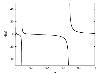
This behaviour goes on and $\hat{g}_{3}$ runs into negative infinity whenever the denominator of Eq. (53) becomes zero. This occurs at the points

\Lambda_{n}=\Lambda_{*}\left(e^{\frac{\pi}{s_{0}}}\right)^{n}\exp\left[\frac{\arctan(s_{0})-\frac{\pi}{2}}{s_{0}}\right],

(59)

where $n$ ’s are integers. We therefore see the emergence of a discrete scale invariance in this three-chain problem even though the melting itself or the three-chain interaction per se has no indication of this sort.

As $\hat{g}_{3}$ can also be interpreted as the three-body binding energy, at those values of $\Lambda$ we get the three-body Efimov bound states in the quantum case. The corresponding energy spectrum of the quantum three-particle system would follow a geometric relation given by

E_{n+1}/E_{n}=e^{-2\pi/s_{0}},

(60)

where $E_{n}$ is the $n$ th energy state. So the energies of the Efimov states are related by a factor of $e^{2\pi/s_{0}}$ . We observe from Eq. (57) that two successive windings around the unit circle are also related through the factor $e^{\pi/s_{0}}$ . As $H$ has nontrivial values at these points we conclude that every jump from one energy level to the next one corresponds to one winding of $\zeta$ around the closed trajectory. It can also be observed that $\hat{g}_{3}$ goes to zero at the points

\Lambda_{n}=\Lambda_{*}\left(e^{\frac{\pi}{s_{0}}}\right)^{n}\exp\left[\frac{\frac{\pi}{2}-\arctan(s_{0})}{s_{0}}\right],

(61)

where the numerator of Eq. $(\ref{theh})$ becomes zero. At these special points we do not have to introduce three-body coupling. So, in this picture every jump corresponds to a switching of one Efimov state to another one and it is associated with a complete winding around a limit cycle. These states are crowded more and more as one goes in the direction of zero energy. They are infinite in number.

To summarize, we see that each of $g_{2}$ and $g_{3}$ , acting alone on its own, allows critical points in the form of melting or dissociation, well described by the conventional renormalization group fixed points. These points show a continuous scale invariance; under a rescaling of the system by any factor, $L\to bL$ for any $b$ , a critical system remains critical, statistically identical. In contrast, at such a fixed point for $g_{2}$ , $g_{3}$ shows a cyclic behaviour, better described as a “limit cycle” behaviour, in the complex plane, because of the emergence of a periodicity. The log periodicity induces a discrete scale invariance, $L\to b_{n}L$ for a discrete set $b_{n}$ , breaking the continuous symmetry expected at the critical value of $g_{2}$ for two chains. In quantum mechanics, this leads to an infinite set of energy eigenstates in a three-particle system at the point where the energy of any pair should have been zero. In the context of DNA, at the melting point of a double stranded DNA where the strands are not bound to each other, a third strand induces a binding of a size much larger than the hydrogen bond length. In other words the infinite correlation length scale of a duplex DNA gets transmuted to a finite value in the presence of a third one when each pair is supposed to be critical.

IV.3 Off-critical: $g_{2}\neq g_{2c}$

So far we have considered the case of the critical two-chain case. For the general situation, $g_{2}\neq g_{2c}$ , we need to go back to Eq. (36), and we also need the flow equation for $g_{2}$ . Instead, we may take a heuristic approach. In terms of the dimensionless two- and three-body constants $\hat{g}_{3},\hat{g}_{2}\sim g_{2}\Lambda^{-1/2}$ , with $H\sim\hat{g}_{3}/\hat{g}_{2}^{2}$ , the expected form of the RG flow equation for $g_{2}$ is

\Lambda\frac{\partial\hat{g}_{2}}{\partial\Lambda}=\beta_{2}(\hat{g}_{2}),

(62)

with an unstable fixed point $\hat{g}_{2}=0$ for the bound phase and a stable one at $\hat{g}_{2}=\hat{g}_{c}$ for the duplex melting. At these points $\beta_{2}(\hat{g}_{2})=0$ . With these, we may formally write

\Lambda\frac{\partial\hat{g}_{3}}{\partial\Lambda}=\frac{2\hat{g}_{3}}{\hat{g}_{2}}\ \beta_{2}(\hat{g}_{2})-4\;\hat{g}_{2}^{2}\;\beta(H,\hat{g}_{2}),

(63)

relating the $\beta$ function for $\hat{g}_{3}$ with the others. As expected, for the duplex melting point with $\beta_{2}(\hat{g}^{*}_{2})=0$ , the flow of $\hat{g}_{3}$ is the same as that of $H$ and therefore $\hat{g}_{3}$ is to be described by the pair of complex fixed points. However, for the $\hat{g}_{2}=0$ fixed point, to get back Eq. (33), $\beta(H)$ of Eq. (54) is not sufficient because it does not yield a $\hat{g}_{2}$ -independent limit. This indicates that the contributions of the off-critical terms in $W$ , Eq. (36), are important. This can be taken as a signal that the periodicity that develops at the duplex melting point for $g_{3}$ or $\hat{g}_{3}$ do not survive in the off-critical limit. A flow diagram is shown in Fig. 8 which depicts a few cycles before merging with the flow at $g_{2}=g_{2c}$ .

V Discussion

At this point we would like to place the results of this paper in a broader context. We do so in three different contexts, namely (i) as a DNA problem, (ii) as an Efimov effect, and (iii) more formally as a renormalization-group problem. Let us first discuss the last two issues, as elaborated upon in the Introduction. The results, in conjunction with the previous works, provide a possible testing ground for the quantum Efimov physics in a classical environment, namely the melting of DNA which occurs at temperatures in the range 60–100C. Here thermal fluctuations play the role of quantum fluctuations [54]. It was shown earlier that the fluctuation induced long range inverse-square attraction has a natural basis in the polymer scaling. Here we showed how the polymer phase transitions in the various limiting situations allowed us to construct an extrapolation formula for the renormalization group $\beta$ function that shows the development of the limit cycle behaviour. This is also important in the general theory of renormalization group where examples of limit cycles are rather few.

Let us now look at it as a DNA problem. The paper builds on the model of a stiff duplex [10] and extends the study of the third virial coefficient of the three-polymer system to the region around the duplex melting point (at temperature $T_{c}$ ). This extension, which goes beyond Ref. [10], shows that the fluctuation-induced Efimov DNA is not just a specialty of the melting point but it also exists over a region where the duplex should have been unbound. Although the fractal-like lattices of Ref. [7, 8, 9] showed the possibility of the three-chain thermodynamic phase, the lack of a metric or distance forbade any analysis of the inverse square law attraction responsible for the Efimov effect. This gap is now partly filled by the analysis of this paper. Short of a direct proof of the inverse-square attraction, the limit cycle behaviour is similar to the complex fixed points known in systems with such long range interaction.

There are several issues which might be amenable to experimental verification. The third strand could be made of alternating short sequences of both the strands. (i) A direct test of the Efimov-effect in DNA would be a measurement of the melting temperature $T_{t}$ of the triple-chain system to see if $T_{t}>T_{c}$ . The melting is expected to be first-order in nature. The difficulty of course lies in separating the melting of the Efimov DNA from that of a Watson-Crick and Hoogsteen paired triple-stranded DNA. (ii) A different thermodynamic study would be the virial coefficients via the osmotic pressure of dilute solutions [55]. The third virial coefficient will give $H(\Lambda)$ , Eq. (8). Near the melting of duplex, the cutoff parameter may be chosen as the bubble length scale $\xi$ , Eq. (26). Therefore, for $\Lambda\sim\xi^{-1}\sim\sqrt{\Delta t}$ , the virial coefficient is expected to show an oscillatory behaviour whose periodicity is determined by the (nonuniversal) Efimov number $s_{0}$ . (iii) More detailed information might be obtained from small angle neutron scattering (SANS) or light scattering. One of the signatures of the fluctuation induced long range interaction is the $1/k$ divergence of $W(k)$ in Eq. (37), since $\overline{W}$ is bounded. Such a divergence in the interaction is observable as a zero- $k$ peak in the scattered intensity in SANS or light scattering [56]. (iv) It is possible to design tailor-made environments where one might test some of the details that have gone in the theory. For example, one may use the geometry of two similar strands maintained at a distance larger than the hydrogen bond length to prevent direct pairing and then allow a complementary strand to form bonds via strand exchange (Fig. 1) with both the strands. The force needed to unzip one of the original strands can then be measured to verify the inverse square nature. Such experiments will be similar in spirit to the measurement of the fluctuation induced Casimir force or the entropic interaction in DNA solution [57, 58]. (v) An assumption that has gone in the theory, actually in most field theoretic calculations (see Ref. [53]), is that the third chain between two contacts with the other two strands is in a relaxed state. This condition may be verified by using a carefully constructed bubble and then placing a third chain. A labeled chain (with say heavier isotopes) will help in separating out the scattering from this chain and provide information on its configuration. (vi) A different experiment would be to study the DNA in a narrow pore. The constraint prevents the large loop formation, thereby cutting off the long range interaction. In this situation, the Efimov-DNA formation is not likely to happen but a novel finite size effect would be expected [59]. The effects would be observable in the configuration of the labeled chain and even in thermodynamic quantities. Such experiments of DNA in a pore has been attempted but not at the level that may explore the large loops near DNA melting [60]. (vii) One may go beyond the three-chain problem to the possibility of a four or more chain bound state, or even a gel formation in a many strand solution through the Efimov interaction. In such a gel, just above the duplex melting point, the mesh size of the network would be similar to the bubble size. A theoretical study of this gelation phenomenon and the elastic properties of the gel remain an open and interesting topic.

VI Conclusion

This paper presents a model of a three-stranded DNA as a three-chain polymer system, which shows mathematically analogous results as that of Efimov physics, namely, the possibility of a three-chain bound state when no two are bound. The existence of a three-stranded DNA bound state (Efimov DNA) at the duplex DNA melting point is shown here analytically by a renormalization group approach. To achieve this, a nonperturbative momentum-shell type RG procedure is employed. We studied the duplex-DNA melting by introducing a rigid chain model, where the melting is induced by an interfacial term. A completely bound two-stranded state at zero temperature is the zero temperature configuration. At finite temperatures thermal fluctuations locally denature the bound state to form bubbles made of two free-chain pairs. A third similar strand, when added, can again form a duplex with one or both of the free chains of a bubble. Due to renormalization of short range interactions close to the duplex melting point an effective long range three-chain interaction is generated. The Efimov DNA is a result of this. Just as in the quantum Efimov problem, we show that the Efimov-DNA is associated with a limit cycle behaviour of the RG flow of the generated three-chain interaction. Since the interaction parameters for a DNA are easily tunable, by choosing solvent quality, we hope our results would motivate experiments in detecting the Efimov effect in polymeric systems.

Appendix A Bound State

The Fourier-Laplace transformed bound state partition function is given by

$\displaystyle Z_{\sf b}({\bf k},s)$	$\displaystyle=$	$\displaystyle\int d\hat{{\bf n}}\int_{0}^{\infty}dNe^{-Ns}$	(64)
		$\displaystyle\hskip 14.22636pt\times\int d^{3}{\bf r}e^{i{\bf k\cdot r}}\frac{e^{-\epsilon N\Lambda^{2}}}{(4\pi)}\delta({\bf r}-N\Lambda\hat{\bf n})$
	$\displaystyle=$	$\displaystyle\int\frac{d\hat{{\bf n}}}{4\pi}\int_{0}^{\infty}dNe^{-Ns}e^{-\epsilon N\Lambda^{2}}e^{iN\Lambda{\bf k\cdot\hat{n}}}$
	$\displaystyle=$	$\displaystyle\frac{1}{2}\int_{0}^{\pi}\frac{\sin\theta d\theta}{s+\epsilon\Lambda^{2}-ik\Lambda\cos\theta}$
	$\displaystyle=$	$\displaystyle\frac{1}{k\Lambda}\arctan\frac{k\Lambda}{s+\epsilon\Lambda^{2}}$

Appendix B Rules Of Diagrammatic Calculations

In this appendix we list all the rules to evaluate diagrams we have used.

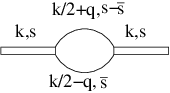
Every partition function has two arguments: one space and one length respectively. With translational invariance, the arguments would be the difference of the corresponding quantities at the two ends of each piece. The dissociation of a bubble or a duplex is our two-body vertex $g_{2}$ [Fig. 2(c) and Fig 3(b)]. The interaction between one single chain and a duplex [Fig 3(c)] is the three-chain vertex $g_{3}$ . The algebraic expression for any diagram is obtained by sequentially multiplying the partition functions and the vertexes as arranged, with integrations over the intermediate variables. A renormalized vertex is called a vertex function.

To see how the $k$ conservation appears, consider a bound state with one bubble of the type in Fig. 9. Applying the above stated rules, this diagram is evaluated as

	$\displaystyle I({\bf r},N)$	$\displaystyle=$	$\displaystyle\int{\sf Z}_{b}({\bf r_{1}}\|z_{1}){\sf Z}^{2}({\bf r_{1}-r_{2}}\|z_{2}-z_{1})$		(65)
			$\displaystyle\times{\sf Z}_{b}({\bf r-r_{2}}\|N-z_{2})d{\bf r_{1}}d{\bf r_{2}}dz_{1}dz_{2}.$		(65)

The convolution form in the real space leads to a product form in the Fourier space. We suppress the $z$ integrals for the time being. Fourier transforming both sides from variable r to k and rewriting right hand partition functions in terms of their Fourier transformed functions we get

$\displaystyle\hat{I}({\bf k},N)$	$\displaystyle=$	$\displaystyle\int I({\bf r},N)e^{-i{\bf k\cdot r}}d{\bf r}$	(66)
	$\displaystyle=$	$\displaystyle\frac{1}{(2\pi)^{4d}}\int Z_{b}({\bf k_{1}}\|z_{1})Z({\bf k_{2}}\|z_{2}-z_{1})Z({\bf k_{3}}\|z_{2}-z_{1})Z_{b}({\bf k_{4}}\|N-z_{2})$
		$\displaystyle\hskip 56.9055pt\times e^{i{\bf r_{1}}\cdot({\bf k_{1}-k_{2}-k_{3}})}e^{i{\bf r_{2}}\cdot({\bf k_{2}+k_{3}-k_{4}})}e^{i{\bf r}\cdot({\bf k_{4}-k})}d{\bf r}\prod_{j=1,2}\{d{\bf r}_{j}dz_{j}\}\prod_{l=1}^{4}d{\bf k}_{l},$
	$\displaystyle=$	$\displaystyle\frac{1}{(2\pi)^{4d}}\int Z_{b}({\bf k_{1}}\|z_{1})Z({\bf k_{2}}\|z_{2}-z_{1})Z({\bf k_{3}}\|z_{2}-z_{1})Z_{b}({\bf k_{4}}\|N-z_{2})\times$
		$\displaystyle\hskip 56.9055pt\delta({\bf k_{1}-k_{2}-k_{3}})\delta({\bf k_{2}+k_{3}-k_{4}})\delta({\bf k_{4}-k})\ dz_{1}dz_{2}\prod_{j=1}^{4}d{\bf k_{j}}.$

Performing three $\delta$ function integrals we get the following relation between different k’s:

\displaystyle{\bf k_{1}=k_{2}+k_{3}},\quad{\bf k=k_{4}},\quad{\bf k_{4}=k_{2}+k_{3}}\quad\mbox{and}\hskip 7.11317pt{\bf k=k_{1}}.

(67)

From these relations it is clear that overall there is one single k and it is conserved at every junction point. Now as there are four unknown ks and we have only three constraints, there is one undetermined k left. This is the characteristic of the loop in the diagram. Whenever there is a loop there is an undetermined k over which we have to integrate ( $\frac{1}{(2\pi)^{d}}\int d{\bf k}$ ). The integration over $\bf k$ corresponds to a bubble in real space with two ends fixed, as, e.g., in $Z^{2}({\bf r_{1}-r_{2}}|z_{2}-z_{1})$ in Eq. (65).

Now we show how the $s$ conservation appears by evaluating Eq. (65). Laplace transforming both sides in $N$ and rewriting every term in the right hand side through their inverse Laplace transformation we have

$\displaystyle A({\bf r},s)$	$\displaystyle=$	$\displaystyle\int_{0}^{\infty}e^{-sN}I({\bf r},N)dN$	(68)
	$\displaystyle=$	$\displaystyle\frac{1}{(2\pi i)^{4}}\int_{0}^{\infty}e^{-sN}dN\int\prod_{j=1,2}\{d{\bf r}_{j}dz_{j}\}\ \prod_{l=1}^{3}ds_{l}\ Z_{\sf b}({\bf r}_{1},s_{1})e^{s_{1}z_{1}}Z({\bf r}_{2}-{\bf r}_{1},s_{2})e^{s_{2}(z_{2}-z_{1})}$
		$\displaystyle\hskip 128.0374pt\times Z({\bf r}_{2}-{\bf r}_{1},s_{2})e^{s_{3}(z_{2}-z_{1})}Z_{\sf b}({\bf r}-{\bf r}_{2},s_{4})e^{s_{4}(N-z_{2})},$

where the $s_{i}$ integrals are the usual Mellin integrals. We evaluate $z$ integrations with limit $z_{1}=0$ to $z_{2}$ , and $z_{2}=0$ to $N$ to get

A({\bf{r}},s)=\int_{0}^{\infty}dN\int_{r_{i},s_{i}}(...)\left[\frac{e^{N(s_{1}-s_{4})}-1}{(s_{1}-s_{4})(s_{1}-s_{2}-s_{3})}-\frac{e^{N(s_{2}+s_{3}-s_{4})}-1}{(s_{2}+s_{3}-s_{4})(s_{1}-s_{2}-s_{3})}\right]e^{(s_{4}-s)N}.

(69)

If we now do the $s_{i}$ integrations using the method of residues, contributions come only from the poles at $s_{1}=s_{4}$ , $s_{1}=s_{2}+s_{3}$ and from the $N$ integration $s=s_{4}$ . As the first bound segment is labeled by $s_{1}$ , two free chains are labeled by $s_{2}$ and $s_{3}$ and the end bound state is labeled by $s_{4}$ , we see the $s$ conservation at every point with an overall $s$ . And similar to the case of k conservation, every loop in Laplace space also possesses one undetermined $s$ as there are three relations and four $s$ ’s to be determined. So whenever a loop comes, we have to integrate over that undetermined $s$ ( $\frac{1}{2\pi i}\int ds$ ).

We can now label the diagram in the Fourier-Laplace space using the above conservation rules as shown in Fig. 9(c). When evaluated algebraically it gives $Z_{b}^{2}({\bf k},s)I_{0}$ with the loop integral

$\displaystyle I_{0}$	$\displaystyle=$	$\displaystyle\int\frac{d\bar{s}}{2\pi i}\frac{d{\bf q}}{(2\pi)^{3}}Z\left(\frac{{\bf k}}{2}-{\bf q},\bar{s}\right)Z\left(\frac{{\bf k}}{2}+{\bf q},s-\bar{s}\right)$	(70)
	$\displaystyle=$	$\displaystyle\int\frac{d\bar{s}}{2\pi i}\frac{d{\bf q}}{(2\pi)^{3}}\ \frac{1}{\bar{s}-\Lambda^{2}\ln\mu+\frac{({\bf k}/2-{\bf q})^{2}}{2}}$
		$\displaystyle\hskip 28.45274pt\times\frac{1}{s-\bar{s}-\Lambda^{2}\ln\mu+\frac{({\bf k}/2+{\bf q})^{2}}{2}}.$

We evaluate the $\bar{s}$ integral by employing the method of residues. There is a simple pole at $\bar{s}=\Lambda^{2}\ln\mu-\frac{({\bf k}/2-{\bf q})^{2}}{2}$ . All the contribution to the integral comes only from this simple pole. So replace the rest of the $\bar{s}$ by its value at the pole and the prefactor $\frac{1}{2\pi i}$ cancels out yielding

	$\displaystyle I_{0}$	$\displaystyle=$	$\displaystyle\int\frac{d{\bf q}}{(2\pi)^{3}}\frac{1}{s{{}^{\prime}}+\frac{k^{2}}{4}+q^{2}}$
		$\displaystyle=$	$\displaystyle\frac{4\pi}{(2\pi)^{3}}\left[\Lambda-\sqrt{s^{\prime}+k^{2}/4}\arctan\frac{\Lambda}{\sqrt{s^{\prime}+k^{2}/4}}\right]$

where $s{{}^{\prime}}=s-2\Lambda^{2}\ln\mu$ . A similar kind of integrals also appear while evaluating three-chain diagrams. We employ this same procedure to evaluate them.

All the diagrams of this paper are evaluated by using the rules and procedures discussed in this appendix.

Appendix C A simple $\beta$ function for $\hat{g}_{3}$

We propose an extrapolation formula that connects smoothly the flows for the $\hat{g}_{2}=0$ case to the $\hat{g}_{2}=\hat{g}^{*}_{2}$ flows. This is a toy example to amplify the limit cycle behaviour in a three-dimensional parameter space, namely, $\hat{g}_{2}$ and the real and imaginary parts of $\hat{g}_{3}$ . For simplicity we choose, $s_{0}=1$ .

Take

\beta(\hat{g}_{2})=\frac{4-d}{2}\hat{g}_{2}-\hat{g}_{2}^{2},

(71)

with an unstable fixed point at $\hat{g}_{2}=0$ and a stable fixed point at $\hat{g}_{2}=1/2$ .

Use this to write for $d=3$ [Eq.(63)]

	$\displaystyle\beta(\hat{g}_{3},\hat{g}_{2})$	$\displaystyle=$	$\displaystyle\hat{g}_{3}-2\hat{g}_{3}\hat{g}_{2}$		(72)
			$\displaystyle-4\hat{g}_{2}^{2}\left(2H-F_{2}(\hat{g}_{2})H^{2}-2H-1\right),$		(72)

where, with $H=-\hat{g}_{3}/(4\hat{g}_{2}^{2})$ as before, the $2H$ term is made explicit for comparison with Eq. (10b), and we defined $F_{2}(\hat{g}_{2})=4\hat{g}_{2}^{2}$ . With these choices, we recover both the limit of $\hat{g}_{2}=0$ and $\hat{g}_{2}=1/2$ the critical melting point.

The flow diagram in the three-dimensional space of $\hat{g}_{2},{\rm{Re}}(\hat{g}_{3}),{\rm{Im}}(\hat{g}_{3})$ shows the approach to the planar cycle at the melting point. This is shown in Fig. 10. So long as the flow is controlled by the real fixed points, we see a monotonic flow. As $\hat{g}_{2}$ changes, the complex fixed points take over and we get the loops.

References

[1] J. D. Watson, Molecular Biology of the Gene, 7th ed. (Pearson, Cold Spring Harbour, NY, 2013).
[2] R. R. Sinden, DNA Structure and Function (Academic, San Diego, CA, 1994).
[3] M. D. Frank-Kamenetskii and S. M. Mirkin, Annu. Rev. Biochem. 64, 65 (1995).
[4] I. Radhakrishnan and D. J. Patel, Biochemistry 33, 11405 (1994).
[5] E. N. Nikolova, E. Kim, A.A. Wise, P.J. O’Brien, I. Andricioaei and H.M. Al-Hashimi, Nature (London) 470 498 (2011).
[6] See, e.g., M. J. Neale and S. Keeney, Nature (London)442, 153 (2006).
[7] J. Maji, S. M. Bhattacharjee, F. Seno, A. Trovato; New J. Phys. 12, 083057 (2010).
[8] J. Maji, S. M. Bhattacharjee, Phys. Rev. E 86, 041147 (2012).
[9] J. Maji, S. M. Bhattacharjee, F. Seno and A. Trovato, Phys Rev E89, 012121 (2014).
[10] T. Pal, P. Sadhukhan and S. M. Bhattacharjee, Phys. Rev. Lett. 110, 028105 (2013) .
[11] V. Efimov, Phys. Lett. B33, 563 (1970).
[12] V. Efimov, Sov. J. Nucl. Phys. 12, 589 (1971).
[13] V. Efimov, Sov. J. Nucl. Phys. 29, 546 (1979).
[14] E. Nielsen, D.V. Fedorov, A.S. Jensen, E. Garrido, Phys. Rept. 347, 373 (2001).
[15] E. Braaten, H. W. Hammer, Phys. Rep. 428, 259 (2006).
[16] O. Gotoh, Adv. Biophys. 16, 1 (1983).
[17] S. M. Bhattacharjee, J. Phys. A 33, L423 (2000); 33, 9003(E) (2000).
[18] P. Sadhukhan and S. M. Bhattacharjee, Ind. J. Physics, 88, 895 (2014).
[19] S. Kumar and and M S Li, Phys. Rep. 486, 1 (2010).
[20] P. G. deGennes, Scaling Concepts in Polymer Physics, (Cornell University Press, Ithaca, 1979).
[21] A. Fonseca, E. Redish, and P. E. Shanley, Nucl. Phys. A320, 273 (1979).
[22] P. F. Bedaque, H. -W. Hammer, U. van Kolck, Nucl. Phys A646, 444 (1999).
[23] Y. Horinouchi and M. Ueda, Phys. Rev. Lett. 114, 025301 (2015).
[24] S. D. Glazek, K. G. Wilson, Phys. Rev. D 48, 5863 (1993); Phys. Rev. Lett. 89, 230401 (2002).
[25] N T Zinner and A S Jensen, J. Phys. G: Nucl. Part. Phys. 40, 053101 (2013).
[26] M. Zaccanti, B. Deissler, C. D’Errico, M. Fattori, M. Jona-Lasinio, S. Müller, G. Roati, M. Inguscio and G. Modugno, Nat. Phys. 5, 586 (2009).
[27] S. Knoop, F. Ferlaino, M. Mark, M. Berninger, H. Schöbel, H. C. Nägerl, R. Grimm, Nat. Phys. 5, 227 (2009).
[28] S. M. Bhattacharjee and S. Mukherji, Phys. Rev. Lett. 83, 2374 (1999).
[29] S. Mukherji and S. M. Bhattacharjee, Phys. Rev. E 63, 051103 (2001).
[30] E. B. Kolomeisky and J. P. Straley, Phys. Rev. B 46, 12664 (1992).
[31] If two random walkers or directed polymers starting at one spatial point rejoin at another point (including the starting point) then it is called a reunion. The corresponding partition function of the bubble decays as a power law in the large length limit, $Z_{R}\sim N^{-\psi_{R}}$ . This exponent $\psi_{R}$ is called the reunion exponent, which plays an important role in determining the order of the melting transitions.
[32] S. Piatecki and W. Krauth, Nature Communications 5, 3503 (2014)
[33] P. Sadhukhan and S. M. Bhattacharjee, J. Phys. A: Math. Theor. 43 245001 (2010); Europhys. Lett. 98, 10008 (2012).
[34] J. J. Rajasekaran and S. M. Bhattacharjee, J. Phys. A24, L371 (1991).
[35] Although it seems that DNA is a one-dimensional object, actually it is not. The dimensionality $d$ of the embedding space in which DNA, and its monomers, live is important in determining physical properties of DNA. This dimension specific to the model of concern can also be changed, e.g., for a DNA on a surface ( $d=2$ ) or a DNA in a solution ( $d=3$ ). So the theorem that there cannot be any phase transition in one dimension is not applicable.
[36] For a debate on what should be the form of a coarse-grained Hamiltonian for DNA, see, e.g., M. D. Frank-Kamenetskii and S Prakash, Physics of life reviews 11, 153 (2014).
[37] A. Son, A.-Y. Kwon, A. Johner, S.-C. Hong and N. Lee, Europhys. Lett. 105, 48002 (2014).
[38] G. A. King, P. Grossa, U. Bockelmann, M. Modesti, G. J. L. Wuitea, and E. J. G. Peterman, Proc. Natl. Acad. Sci. U.S.A. 110, 3859 (2013).
[39] J.-H. Jeon and W. Sung, Biophys J. 95, 3600 (2008).
[40] T. R. Strick, J. F. Allemand, D. Bensimon, and V. Croquette, Proc. Natl. Acad. Sci. U.S.A. 95, 10579 (1998).
[41] J. H. Jeon, J. Adamcik, G. Dietler and R. Metzler, Phys. Rev. Let. 105, 208101 (2010).
[42] G. Altan-Bonnet, A. Libchaber and O. Krichevsky, Phys. Rev. Lett. 90, 138101 (2003).
[43] T. Ambjörnsson, S. K. Banik, O. Krichevsky, R. Metzler, Phys. Rev. Let. 97, 128105 (2006).
[44] B. S. Alexandrov, Y. Fukuyo, M. Lange, N. Hirikoshi, V. Gelev, K.Ø. Rasmussen, A.R. Bishop and A. Usheva, Nucl. Acids Res. 40, 10116 (2012).
[45] F. Sicard, N. Destainville and M. Manghi, J. Chem. Phys. 142, 034903 (2015).
[46] R. Kapri, Phys. Rev. E 90, 062719 (2014).
[47] S. Kumar and G. Mishra, Phys. Rev. Lett. 110, 258102 (2013).
[48] J. H. Jeon, W. Sung, F. H. Ree, J. Chem. Phys. 124, 164905 (2006).
[49] The three-chain coupling $g_{3}$ here is the negative of the same parameter in Ref. [10]. This is done for easy comparison with polymer formulations of Refs. [34, 28, 29].
[50] The expression for $\Delta t$ can be written in a general form as

$\Delta t=\left[Z_{\sf b}^{-1}(s^{\prime}\to 0,{\bf k}\to 0)-4\pi g_{2}^{2}\Lambda\right]\ \Lambda^{-2}.$
[51] M. E. Fisher, J. Stat. Phys 34, 667 (1984).
[52] For three different chains, if we label the interface weight as $g_{2}^{ij}$ for pair $i,j$ , then the strand exchange would be like $g_{2}^{12}g_{2}^{23}+g_{2}^{13}g_{2}^{23}$ . As we are considering all the interface weights as $g_{2}$ , the factor of $2$ comes in.
[53] This condition is similar to the “on-shell” condition used in field theory. In field theoretical calculations on-shell and off-shell conditions referred to the center-of-mass frame or non-center-of-mass frame respectively. Our notion of a relaxed DNA segment is similar to the on-shell condition where only the Gaussian part ( $\sim q^{2}$ ) is important. For off-shell considerations one needs to consider non-Gaussian terms (higher order terms in $q$ ) which we ignore in this paper.
[54] Other known examples of this type are nonrelativistic solid state phyics problems providing examples of relativistic quantum mechanics, liquid crystals as testing ground of cosmological theories; see Ref. [10].
[55] T. Oohashi, K. Inoue and Y. Nakamura, Polymer J. 46, 699 (2014).
[56] The rise in the scattered intensity at very small wave vectors in small angle neutron scattering has been used to identify effective long range attraction between protein molecules in solutions. See, e.g.,Y. Liu, E. Fratini, P. Baglioni, W. R. Chen, and S. H. Chen, Phys. Rev. Lett. 95, 118102 (2005).
[57] U. Mohideen and A. Roy, Phys. Rev. Lett. 81, 4549 (1998).
[58] R. Verma, J. C. Crocker, T. C. Lubensky, and A. G. Yodh, Phys. Rev. Lett. 81, 4004 (1998).
[59] A. Grosberg, Physics of Life Reviews 11, 178 (2014).
[60] W. Reisner, N.B. Larsen, A. Silahtaroglu, A. Kristensen, N. Tommerup, J.O. Tegenfeldt and H. Flyvbjerg, Proc. Natl. Acad. Sci. U.S.A. 107, 13294 (2010).