Di-Higgs phenomenology: The forgotten channel
Abstract
Searches for multi-Higgs final states allow to constrain parameters of the SM (or extensions thereof) that directly relate to the mechanism of electroweak symmetry breaking. Multi-Higgs production cross sections, however, are small and the phenomenologically accessible final states are challenging to isolate in the busy multi-jet hadron collider environment of the LHC run 2. This makes the necessity to extend the list of potentially observable production mechanisms obvious. Most of the phenomenological analyses in the past have focused on ; in this paper we study at LHC run 2 and find that this channel for and semi-leptonic and hadronic top decays has the potential to provide an additional handle to constrain the Higgs trilinear coupling in a global fit at the end of run 2.
I Introduction
The Higgs discovery in 2012 by the ATLAS and CMS experiments [1, 2] and subsequent preliminary comparisons of its properties against the Standard Model (SM) expectation [3] have highlighted its SM character in standard measurements. The next step in demystifying the nature of the electroweak scale will therefore crucially rely on precise measurements of the Higgs’ properties at low as well as high momentum transfers during run 2, and on constraining or even measuring Higgs properties that have not been in the sensitivity reach during run 1.
A parameter in the SM that is directly sensitive to spontaneous symmetry breaking is the quartic Higgs coupling
| (1) |
where we use the unitary gauge and . The second independent parameter in the SM Higgs potential is reverse–engineered to obtain an acceptably large value of the electroweak symmetry breaking scale and pole mass
| (2) |
for a given Higgs self-coupling . These relations determine a unique value of the Higgs self-coupling in the SM as required by renormalisablility.
To obtain a measurement of the Higgs self-coupling , we may think of Eq. (1) as the lowest order in an effective field theory expansion in a new physics scale . A new operator possibly relevant for softening the correlation of Higgs mass and electroweak scale is, e.g., . Consequently, in the absence of additional new resonant phenomena related to electroweak symmetry breaking and in order to prove or disprove the existence of such operators, a question that needs to be addressed is how well the Higgs self-interaction parameter can be constrained assuming the standard low-energy Higgs phenomenology only.
Our best option to phenomenologically access the relevant parameter at the LHC is via its impact on di-Higgs production [4, 5] via the trilinear Higgs self-coupling. Inclusive di-Higgs cross sections typically have cross sections in the (10 fb) range [6, 7]. This implies that, in order to analyse them, the large SM-like Higgs branching ratios [8, 9, 10] and [11] must be employed. Advanced substructure techniques [12, 13] or small irreducible backgrounds such as in [14, 15] are crucial in most analyses to date, which have focused on the dominant di-Higgs production cross section, gluon fusion (GF) with [16]. To increase sensitivities in this channel emission of an additional jet has been discussed in Refs. [8, 17]; a complete analysis of WBF-like production in has become available only recently [18].
Common to all realistic di-Higgs analyses discussed in the literature is that they will be sensitive to systematic uncertainties at the end of run 2 and it is quite likely that measurements in only a single di-Higgs channel will not provide enough information to formulate a significant constraint on the Higgs self-interaction in the above sense [19]. Hence, it is mandatory to extend the list of potential phenomenologically interesting search channels in proof-of-principle analyses.
In this paper we investigate , and study semi-leptonic and hadronic top decays and . In particular, we discuss the phenomenological appeal of this particular di-Higgs final state as a function of the number of applied -tags. We first study the qualitative behaviour of in Sec. II, where we also comment on the signal and background event generation employed in the remainder of this work. In Sec. III, we detail our analysis and we discuss the sensitivity of to in detail before we present our conclusions in Sec. IV.
II Signal Cross Section Sensitivity and Event Generation
The sensitivity of di-Higgs cross sections from GF and WBF is dominated by destructive interference of the continuum production and the subamplitude containing proportional to the trilinear coupling . In gluon fusion this is apparent from low-energy effective theory arguments [20] by expanding
| (3) |
which makes the relative minus between the continuum and the diagrams explicit. As a consequence, the gluon fusion cross section is a decreasing function with . In WBF the destructive character is explicit from nested cancellations that are similar to unitarity-based cancellations observed in longitudinal gauge boson scattering.
Qualitatively different from GF- and WBF-induced di-Higgs production, is the leading cross section which is impacted by constructive interference, yielding an increasing cross section with , Fig. 1. Quite different to loop-induced gluon fusion di-Higgs production, there is no characteristic threshold scale involved in that can be exploited in a targeted boosted search strategy [8, 9]; the cross section is a rather flat function of [6] and differential distributions away from production threshold do not show a significant deviation apart from a global rescaling of the differential distribution by for a transverse momentum range that is interesting for the experiments (Fig. 1). Furthermore, the expected inclusive cross section with at a 14 TeV LHC asks for a selection as inclusive as possible to be sensitive to the signal contribution even for a target luminosity of 3/ab in the first place.
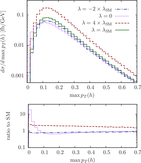
If we treat the top-Yukawa interaction as legacy measurement and set , we can imagine a physics situation with an enhanced trilinear coupling that renders the dominant gluon fusion modes suppressed but leaves an excess in production. In the general dimension six extension alluded to in the introduction this corresponds to a negative Wilson coefficient of . Enhanced Higgs self-couplings have been discussed more concretely in the context of conformal Coleman-Weinberg-type extensions of the SM in [21]. Obviously, the opposite phenomenological situation of is accompanied by enhanced GF and WBF di-Higgs cross sections while becomes smaller (however the cross section becomes rather flat). Such a situation occurs for instance in composite Higgs scenarios [5], which typically have a smaller Higgs trilinear coupling than predicted in the SM (in addition to modified top Yukawa interactions). Therefore, comparing the measured rates and (ideally) distributions in all three channels, i.e. gluon-fusion, weak-boson-fusion and in association with a top quark pair, provides a precision tool for BSM electroweak symmetry breaking.
| signal | backgrounds | |||||||
|---|---|---|---|---|---|---|---|---|
| trigger | 0.10 | 0.23 | 4.75 | 1.38 | 0.64 | 1.37 | 1.36 | 1.33 |
| jet cuts | 7.40 | 0.17 | 1.44 | 0.76 | 0.40 | 0.65 | 8.74 | 7.46 |
| 5 tags | 1.23 | 2.83 | 4.46 | 6.19 | 7.24 | 4.43 | 1.25 | 5.35 |
| 7.33 | 1.69 | 1.59 | 2.71 | 3.41 | 1.56 | 4.28 | 1 | |
| lep./had. | 5.04 | 1.12 | 9.50 | 1.66 | 2.29 | 9.42 | 2.69 | 1 |
| lep. only | 2.33 | 5.29 | 5.03 | 9.36 | 1.14 | 4.90 | 1.39 | 1 |
| had. only | 2.71 | 5.93 | 4.47 | 7.20 | 1.16 | 4.44 | 1.30 | 1 |
| 6 tags | 2.21 | 4.97 | 3.80 | 8.01 | 9.57 | 5.10 | 1.86 | 1 |
| 1.81 | 5.94 | 2.01 | 5.47 | 6.60 | 3.28 | 1.11 | 1 | |
Given the small production cross sections, we focus in the following on semi-leptonic decays of the final state top pair, with both Higgs bosons decaying . We use Sherpa v2.1.1 with the Comix matrix element generator [22] to generate signal and background events for modified trilinear Higgs couplings with SM-like top Yukawa interactions and normalise to the signal events to the NLO cross section of Ref. [6]. The signal and background samples have been generated at purely leading order matched to the parton shower, with modelling of hadronisation effects and underlying event. Unstable particles are treated in the narrow width approximation with the subsequent decays conserving any spin correlations.
III at LHC run 2

III.1 Final State Reconstruction
While this high-multiplicity final state might allow to trigger in multiple ways, due to the low- thresholds for the jets we rely for this purpose on an isolated lepton (muon or electron) with GeV. We define a lepton to be isolated if the hadronic energy deposit within a cone of size is smaller than of the lepton candidate’s transverse momentum and .
After removing the isolated leptons from the list of input particles () of the jet finder we reconstruct jets with and using the anti- algorithm [25] of FastJet [26]. We veto events with less than 6 reconstructed jets.
Out of the 6 jets we require at least 5 to be -tagged by matching the -meson before the decay to the jet. We assume a -tagging efficiency of and a fake rate of [27].
As the signal rate after these inclusive cuts is already fairly small, fb for , we select the Higgs-decay jets by minimising
| (5) |
where run over all -tagged jets and GeV (we comment on this choice further below) and GeV. For the combination which minimises we require and . We then remove these 4 -tagged jets from the event.
To confidently reduce the large gauge boson induced backgrounds, e.g. +jets, we further require at least one top quark to be reconstructed. We provide cross sections after the reconstruction of the leptonic top only, after reconstructing the hadronic top quark only or after reconstructing either the leptonic or the hadronic top quark.
To avoid biasing the vector boson backgrounds towards the top quark signal, for the leptonic top quark reconstruction we require that the invariant mass of the sum of the lepton, a -jet and the missing transverse energy vector, built from all visible objects within , fulfil
| (6) |
with GeV and GeV. To identify the -jet for we consider all remaining -jets in the event and minimise
| (7) |
Similarly, for the hadronic top quark reconstruction we loop over all remaining jets and minimise
| (8) |
We then request
| (9) |
The cut flow for the described analysis steps is shown in Tab. 1.
III.2 Discussion

At a center-of-mass energy of TeV, the signal cross section for is in the sub-femtobarn range before decays are included. Therefore, the reconstruction requires an approach that on the one hand retains an as large as possible signal yield and on the other hand triggers in the high-luminosity regime. We therefore focus on the Higgs decays to bottom quarks and semi-leptonic decays. Other channels can be combined with the one we focus on to improve the sensitivity on measuring the self-coupling.
Already after fulfilling the trigger requirement, minimal jet cuts and 5 tags we find for the backgrounds we consider. To confirm the measurement of a di-Higgs event both Higgs bosons have to be fully reconstructed. At this stage we find with 5 tags and with 6 tags respectively. We show the reconstructed masses of the hardest and second hardest Higgs boson in Fig. 2. Due to the partly invisible decay of B-mesons, is systematically shifted to slightly lower values. This is why we choose GeV for the minimisation procedure. In measurements, the experiments can compensate for this systematic shift in the invariant Higgs mass using -jet calibrations. Further, at this point with the chosen b-tagging-efficiency working point +jets backgrounds are already subleading. Thus, choosing a higher -tagging efficiency working point at cost of a larger fake rate could be beneficial in this analysis to retain a larger signal yield and improve the statistical significance expressed in .
In a further step we then perform a leptonic or hadronic top quark reconstruction using the remaining measured final state objects. This can help to further suppress potentially large reducible QCD-induced backgrounds, e.g. +jets. However, for the top-rich irreducible backgrounds we focus here mostly on, an improvement in cannot be achieved using the signal-sparing minimisation we apply.
From Tab. 1 it becomes obvious that the signal vs. background ratio is expected to be in the range for . After 3/ab we expect 13 signal events including the reconstruction of a top quark and 22 signal events reconstructing only the two Higgs bosons. While the signal yield is too small to claim a discovery at this stage the number of observed events is high enough to formulate an expected 95% confidence level limit on assuming . In order to do this, we employ the CLs method [28, 29] inputting the expected number of signal and background events for a luminosity of 3/ab including the reconstruction of at least one top quark. The result is shown in Fig. 3; and we obtain
| (10) |
IV Summary and Conclusions
With current Higgs property measurements strongly indicating a SM-like character of the discovered Higgs boson, analysis strategies for parameters relevant for electroweak symmetry breaking that remain unconstrained in standard Higgs searches will play a central role in the search for new physics beyond the SM during run 2. Constraining the Higgs self-interaction as one of the most interesting couplings in this regard is a experimentally challenging task and will require a large accumulated data set.
As we have discussed in this letter, the role of production in this regard is twofold: Firstly, it provides an additional channel that can be added to a global Higgs self-coupling analysis across the phenomenologically viable channels. Signal vs. background ratios indicate that top-pair associated Higgs pair production can provide significant statistical power to increase the sensitivity to this crucial coupling at a targeted 3/ab and extend the sensitivity coverage to the Higgs trilinear coupling. Secondly, if we face a situation with , provides the leading channel, where we can expect to observe an excess over the SM expectation. A negative search outcome in GF and WBF dominated search strategies in addition to an excess in final states would therefore be a strong indication of , eventually allowing us to put strong constraints on BSM scenarios such as composite Higgs models.
Acknowledgements. CE is supported by the Institute for Particle Physics Phenomenology Associateship programme.
References
- [1] The ATLAS Collaboration, Phys. Lett. B 716 (2012) 1.
- [2] The CMS Collaboration, Phys. Lett. B 716 (2012) 30.
- [3] The CMS Collaboration, JHEP 06 (2013) 081. The ATLAS Collaboration, arXiv:1307.1427 [hep-ex].
- [4] E. W. N. Glover and J. J. van der Bij, Nucl. Phys. B 309 (1988) 282. D. A. Dicus, C. Kao and S. S. D. Willenbrock, Phys. Lett. B 203 (1988) 457. T. Plehn, M. Spira and P. M. Zerwas, Nucl. Phys. B 479 (1996) 46 [Erratum-ibid. B 531 (1998) 655]. A. Djouadi, W. Kilian, M. Muhlleitner and P. M. Zerwas, Eur. Phys. J. C 10 (1999) 45. S. Dawson, S. Dittmaier and M. Spira, Phys. Rev. D 58 (1998) 115012.
- [5] R. Grober and M. Mühlleitner, JHEP 1106 (2011) 020. R. Contino, M. Ghezzi, M. Moretti, G. Panico, F. Piccinini and A. Wulzer, JHEP 1208 (2012) 154.
- [6] R. Frederix, S. Frixione, V. Hirschi, F. Maltoni, O. Mattelaer, P. Torrielli, E. Vryonidou and M. Zaro, Phys. Lett. B 732 (2014) 142.
- [7] J. Baglio, A. Djouadi, R. Gröber, M. M. Mühlleitner, J. Quevillon and M. Spira, JHEP 1304 (2013) 151.
- [8] M. J. Dolan, C. Englert and M. Spannowsky, JHEP 1210 (2012) 112.
- [9] A. J. Barr, M. J. Dolan, C. Englert and M. Spannowsky, Phys. Lett. B 728 (2014) 308.
- [10] D. E. Ferreira de Lima, A. Papaefstathiou and M. Spannowsky, JHEP 1408 (2014) 030.
- [11] A. Papaefstathiou, L. L. Yang and J. Zurita, Phys. Rev. D 87 (2013) 011301.
- [12] J. M. Butterworth, A. R. Davison, M. Rubin and G. P. Salam, Phys. Rev. Lett. 100 (2008) 242001. T. Plehn, G. P. Salam and M. Spannowsky, Phys. Rev. Lett. 104 (2010) 111801.
- [13] L. G. Almeida, S. J. Lee, G. Perez, G. F. Sterman, I. Sung and J. Virzi, Phys. Rev. D 79, 074017 (2009); D. E. Soper and M. Spannowsky, JHEP 1008, 029 (2010); J. Thaler and K. Van Tilburg, JHEP 1103, 015 (2011); D. E. Soper and M. Spannowsky, Phys. Rev. D 84, 074002 (2011); L. G. Almeida, O. Erdogan, J. Juknevich, S. J. Lee, G. Perez and G. Sterman, Phys. Rev. D 85, 114046 (2012); S. D. Ellis, A. Hornig, T. S. Roy, D. Krohn and M. D. Schwartz, Phys. Rev. Lett. 108, 182003 (2012); D. E. Soper and M. Spannowsky, Phys. Rev. D 87, no. 5, 054012 (2013).
- [14] U. Baur, T. Plehn and D. L. Rainwater, Phys. Rev. D 67, 033003 (2003). U. Baur, T. Plehn and D. L. Rainwater, Phys. Rev. D 69, 053004 (2004).
- [15] The ATLAS Collaboration, ATL-PHYS-PUB-2012-004.
- [16] D. Y. Shao, C. S. Li, H. T. Li and J. Wang, arXiv:1301.1245 [hep-ph]. D. de Florian and J. Mazzitelli, Phys. Lett. B 724 (2013) 306. J. Grigo, J. Hoff, K. Melnikov and M. Steinhauser, arXiv:1305.7340 [hep-ph]. D. de Florian and J. Mazzitelli, arXiv:1309.6594 [hep-ph].
- [17] P. Maierhöfer and A. Papaefstathiou, JHEP 1403 (2014) 126.
- [18] M. J. Dolan, C. Englert, N. Greiner and M. Spannowsky, Phys. Rev. Lett. 112 (2014) 101802.
- [19] F. Goertz, A. Papaefstathiou, L. L. Yang and J. Zurita, JHEP 1306 (2013) 016.
- [20] J. R. Ellis, M. K. Gaillard and D. V. Nanopoulos, Nucl. Phys. B 106 (1976) 292. M. A. Shifman, A. I. Vainshtein, M. B. Voloshin and V. I. Zakharov, Sov. J. Nucl. Phys. 30 (1979) 711 [Yad. Fiz. 30 (1979) 1368]. B. A. Kniehl and M. Spira, Z. Phys. C 69 (1995) 77.
- [21] S. Abel and A. Mariotti, arXiv:1312.5335 [hep-ph].
- [22] T. Gleisberg, S. Hoeche, F. Krauss, M. Schonherr, S. Schumann, F. Siegert and J. Winter, JHEP 0902 (2009) 007. T. Gleisberg, S. Hoeche JHEP 0812 (2008) 039
- [23] M. Guzzi, P. Nadolsky, E. Berger, H. Lai, F. Olness, C.-P.Yuan arxiv:1101.0561 [hep-ph]
- [24] S. Hoeche, F. Krauss, S. Schumann, F. Siegert JHEP 05 (2009) 053. S. Hoeche, F. Krauss, M. Schoenherr, F. Siegert Phys. Rev. Lett. 110 (2013) 052001
- [25] M. Cacciari, G. P. Salam and G. Soyez, JHEP 0804 (2008) 063.
- [26] M. Cacciari, G. P. Salam and G. Soyez, Eur. Phys. J. C 72 (2012) 1896.
- [27] The ATLAS collaboration, ATLAS-CONF-2012-043.
- [28] A. L. Read, CERN-OPEN-2000-205. A. L. Read, J. Phys. G G28 (2002) 2693-2704.
- [29] T. Junk, Nucl. Instrum. Meth. A 434 (1999) 435. T. Junk, CDF Note 8128 [cdf/doc/statistics/public/8128]. T. Junk, CDF Note 7904 [cdf/doc/statistics/public/7904].