Superconducting pairing mediated by spin-fluctuations from first principles

F. Essenberger Affiliation: Max Planck Institute of Microstructure Physics, Weinberg 2, D-06120 Halle, Germany. A. Sanna Affiliation: Max Planck Institute of Microstructure Physics, Weinberg 2, D-06120 Halle, Germany. A. Linscheid Affiliation: Max Planck Institute of Microstructure Physics, Weinberg 2, D-06120 Halle, Germany. F. Tandetzky Affiliation: Max Planck Institute of Microstructure Physics, Weinberg 2, D-06120 Halle, Germany. G. Profeta Affiliation: Consiglio Nazionale delle Ricerche - Superconducting and Innovative Materials and Devices (CNR-SPIN), 67100 L’Aquila, Italy P. Cudazzo Affiliation: Nano-Bio Spectroscopy group, Dpto. Física de Materiales, Universidad del País Vasco, Centro de Física de Materiales CSIC-UPV/EHU-MPC and DIPC, Av. Tolosa 72, E-20018 San Sebastián, Spain Affiliation: European Theoretical Spectroscopy Facility (ETSF) E.K.U. Gross Affiliation: Max Planck Institute of Microstructure Physics, Weinberg 2, D-06120 Halle, Germany.

August 24, 2026

Abstract

We present the derivation of an ab-initio and parameter free effective electron-electron interaction that goes beyond the screened RPA and accounts for superconducting pairing driven by spin-fluctuations. The construction is based on many body perturbation theory and relies on the approximation of the exchange-correlation part of the electronic self-energy within time dependent density functional theory. This effective interaction is included in an exchange correlation kernel for superconducting density functional theory, in order to achieve a completely parameter free superconducting gap equation. First results from applying the new functional to a simplified two-band electron gas model are consistent with experiments.

I Introduction

In the last 30 years the field of superconductivity has been revolutionized by the discovery of high-temperature (hi-T_c) superconductivity (SC). First the Cuprates were found in the 80s[1, 2] and then iron based compounds in the 2000s[3, 4, 5]. Numerous empirical/semi-empirical theoretical models have been developed in order to grasp the essential physics of these materials[6, 7, 8] and still the community is far from a general consensus on the origin of the pairing mechanism. In our opinion consensus can only be achieved in one single way: By developing a universal predictive theory of (hi-T_c) SC that is fully parameter free and is able to reproduce the essential properties of the SC (including its critical temperature, complex gap function and excitation spectrum), under the only knowledge of the atomic constituents and chemical structure.

Within the class of conventional (meaning phonon driven) SC, density functional theory for the SC state (SCDFT) [9], within the available functional[10, 11], proved to be predictive and reliable[12, 13, 14, 15, 16, 17, 18, 19, 20, 21]. However, since the pairing in the pnictides and cuprates is non-phononic[22, 23], this SCDFT approach is not directly applicable, due to the limitations of the functional.

In this work we carefully reconsider this functional and it’s construction, in particular the treatment of the electronic component of the pairing. We aim to reach two goals in this work: The first is very general and not bound to SCDFT applications. We want to formulate a screened effective electron-electron interaction that goes beyond the $GW$ form and includes additional physical effects not present in the random phase approximation (RPA) type of screening. In particular we aim to include the effect of low energy spin-fluctuations, in a computationally feasible way and completely ab-initio (i.e. without the use of parameters - like a Stoner exchange splitting). We focus on the spin-fluctuations because they are one of the prime candidates responsible for SC pairing in iron SC [24]; The second goal we aim for is to cast this effective interaction along the standard Coulomb and phonon contribution[10] in a functional that can be used within the ab-initio SCDFT framework.

The paper has the following outline: In the next section (Sec. II) we discuss briefly the existing functionals of SCDFT. Then we propose the set of relevant diagrams for representing the spin-fluctuations (Sec. III.1) and the corresponding self-energy contribution are constructed in the Nambu formalism (Sec. III.2). After some additional approximation (Sec. III.3) the final form of the self-energy taking the spin-fluctuations into account is presented in Sec. IV. This self-energy may be used also in many-body theory but the focus of this work lies on SCDFT and hence in Sec. V a functional is derived using the Sham-Schlüter connection. In the last part of the present work (Sec. VI) the functional is applied to a two band model system and the trends with respect to the Coulomb, phonon and spin-fluctuations (SF) contributions are investigated.

II A brief review of SCDFT

Before engaging in the task of constructing the effective interaction and the corresponding functional, we briefly review the SCDFT framework and the available functionals. SCDFT is based on a theorem of Oliveira, Gross and Kohn[9], that extends the Hohenberg-Kohn proof[25] of the 1-1 correspondence between density and external potential to the SC density

\chi\left(\boldsymbol{r},\!\boldsymbol{r}^{\prime}\right)=\langle\hat{\varPsi}_{\downarrow}(\boldsymbol{r})\hat{\varPsi}_{\uparrow}(\boldsymbol{r}^{\prime})\rangle

where $\hat{\Psi}_{\sigma}\left(\boldsymbol{r}\right)$ are the usual electronic field operators and $\left\langle\right\rangle$ is the thermal average. The modern version of the theory has been re-formulated by Lüders, Marques and coworkers[10, 18]. This formulation includes an explicit ionic density and a further extension of the Hohenberg-Kohn proof in the spirit of the multicomponent DFT introduced by Kreibich and Gross[26].

In their work, Lüders, Marques and coworkers[10, 18] proposed an exchange-correlation functional derived from many-body perturbation theory and presented solutions of the SC Kohn-Sham (KS) system for real SC. The starting point is an approximation for the self-energy. In their work they use:

	$\displaystyle\bar{\varSigma}_{k}\left(\omega_{n}\right)$	$\displaystyle\approx\sum_{m}\sum_{k^{\prime}}W_{kk^{\prime}}\left(\omega_{n}-\omega_{m}\right)\bar{G}_{k^{\prime}}^{{\scriptscriptstyle\text{KS}}}\left(\omega_{m}\right)$		(1)
		$\displaystyle+\sum_{m}\sum_{k^{\prime}}\varLambda_{kk^{\prime}}^{{\scriptscriptstyle\text{Ph}}}\left(\omega_{n}-\omega_{m}\right)\bar{G}_{k^{\prime}}^{{\scriptscriptstyle\text{KS}}\text{ }}\left(\omega_{m}\right),$		(2)

where $\bar{G}_{k}^{\text{${\scriptscriptstyle KS}$}}\left(\omega_{n}\right)$ is the Green’s function of the SC Kohn-Sham system, in Nambu notation [27], $W_{kk^{\prime}}\left(\omega_{n}\right)$ is the screened Coulomb interaction and $\varLambda_{kk^{\prime}}^{{\scriptscriptstyle\text{Ph}}}$ is the interaction mediated by phonons. We will indicate objects in Nambu notation with a bar (for example $\bar{G}$ ). The components of the Green’s function read:

\bar{G}_{k}\left(\omega_{n}\right)=\uptau^{\mathrm{z}}\begin{pmatrix}G_{k}\left(\omega_{n}\right)&F_{k}\left(\omega_{n}\right)\\ {F_{k}}^{\dagger}\left(\omega_{n}\right)&{G_{k}}^{\dagger}\left(\omega_{n}\right)\end{pmatrix}.

(3)

The $\omega_{n}$ are the fermionic Matsubara frequencies, $k$ is a combined index $k=\left\{n\boldsymbol{k}\right\}$ containing the band index and the momentum of the KS electron and $\uptau^{\mathrm{z}}$ is the third Pauli matrix. The normal ( $G_{k}$ ) and anomalous ( $F_{k})$ part of the Nambu Green’s function are given by:

	$\displaystyle G_{k}\left(\omega_{n}\right)$	$\displaystyle=-\int_{0}^{\beta}\mathrm{d}\tau\mathrm{e}^{\mathrm{i}\omega_{n}\tau}\left\langle\hat{\mathrm{T}}\left[\hat{a}_{k}\left(\tau\right)\hat{a}_{k}^{\dagger}\left(0\right)\right]\right\rangle$
	$\displaystyle F_{k}\left(\omega_{n}\right)$	$\displaystyle=-\int_{0}^{\beta}\mathrm{d}\tau\mathrm{e}^{\mathrm{i}\omega_{n}\tau}\left\langle\hat{\mathrm{T}}\left[\hat{a}_{k}\left(\tau\right)\hat{a}_{k}\left(0\right)\right]\right\rangle$

where $\hat{a}_{k}\left(\tau\right)$ and $\hat{a}_{k}^{\dagger}$ are the usual creation and annihilation operators in the Heisenberg picture, $\hat{\mathrm{T}}$ is the time ordering operator and $\left\langle\right\rangle$ denotes the thermal average. The electronic part of the interaction, in the work of Marques and Lüders, is assumed to be given by the classical (test-charge to test-charge) screened Coulomb interaction[28], therefore it can be expressed in terms of the dielectric function $\epsilon^{-1}$ :

W_{k_{1}k_{2}}\left(\omega_{n}\right)=\sum_{k^{\prime}}\epsilon_{k_{1}k^{\prime}}^{-1}\left(\omega_{n}\right)v_{k^{\prime}k_{2}}

(4)

where $v_{k_{1}k_{2}}$ is the bare Coulomb interaction. The interaction mediate by phonons $\varLambda_{kk^{\prime}}^{{\scriptscriptstyle\text{Ph}}}\left(\omega_{n}\right)$ depends on the electron-phonon coupling matrix elements $g_{\lambda\boldsymbol{q}}^{kk^{\prime}}$ and the phonon frequencies $\varOmega_{\lambda\boldsymbol{q}}$ :

	$\displaystyle\varLambda_{kk^{\prime}}^{{\scriptscriptstyle\text{Ph}}}\left(\omega_{n}\right)$	$\displaystyle=-\frac{1}{\uppi}\int_{0}^{\infty}\!\!\!\mathrm{d}\omega\frac{2\omega}{\omega_{n}^{2}+\omega^{2}}\mathfrak{Im}\left[\varLambda_{kk^{\prime}}^{{\scriptscriptstyle\text{Ph}}}\left(\omega\right)\right]$		(5)
	$\displaystyle\mathfrak{Im}\left[\varLambda_{kk^{\prime}}^{{\scriptscriptstyle\text{Ph}}}\left(\omega\right)\right]$	$\displaystyle=-\uppi\sum_{\lambda\boldsymbol{q}}\left\|g_{\lambda\boldsymbol{q}}^{kk^{\prime}}\right\|^{2}\updelta\left(\omega-\varOmega_{\lambda\boldsymbol{q}}\right).$

A Feynman diagram schematic form for this approximation is shown in Eq. II. For the two terms we use the names $\bar{\varSigma}^{{\scriptscriptstyle GW}}$ and $\bar{\varSigma}^{{\scriptscriptstyle\text{Ph}}}$ , respectively.

Once an approximation for the self-energy is fixed, it is possible to construct the corresponding exchange-correlation (xc) potential using the Sham-Schlüter connection (see Sec. V for details). A key approximation in order to reduce the numerical complexity of SCDFT is the so-called decoupling approximation[29] i.e.

\varDelta_{kk^{\prime}}^{\text{xc}}\approx\updelta_{kk^{\prime}}\varDelta_{k}^{\text{xc}}

that can be interpreted as the exclusion of hybridization effects between the non SC Kohn-Sham orbitals by the effect of the SC condensation. In this approximation the electronic KS system can be diagonalized analytically leading to a self-consistent expression for the pairing potential $\varDelta_{k}^{\text{xc}}$ known as the SCDFT gap equation:

\varDelta_{k}^{\text{xc}}=-\varDelta_{k}^{\text{xc}}\mathcal{Z}_{k}^{\mathrm{{\scriptscriptstyle D}}}-\sum_{k^{\prime}}\mathcal{K}_{kk^{\prime}}^{\mathrm{{\scriptscriptstyle C}}}\frac{\tanh\left(\frac{\beta E_{k^{\prime}}}{2}\right)}{2E_{k^{\prime}}}\varDelta_{k^{\prime}}^{\text{xc}}

(6)

that has the BCS form[30]. The kernels $\mathcal{Z}_{k}^{\mathrm{{\scriptscriptstyle D}}}$ and $\mathcal{K}_{kk^{\prime}}^{\mathrm{{\scriptscriptstyle C}}}$ depend on the temperature, the interaction matrix elements $\left(w_{k_{1}k_{2}},\varLambda_{kk^{\prime}}^{{\scriptscriptstyle\text{Ph}}}\right)$ , the single particle KS energies $\epsilon_{k}$ and $E_{k}:=\sqrt{\left|\varDelta_{k}\right|^{2}+\left(\epsilon_{k}-\mu\right)^{2}}$ . The critical temperatures predicted within this equation agree extremely well with the experimentally observed ones within the class of phononic SC[18, 12, 15, 14, 13, 31, 21, 32]. However, Eq. 6 fails to describe high temperature SC[5, 33], where the SC mechanism is believed to be related to magnetic interactions.

In the next sections we will see that this fact is actually not surprising. One assumption in using a dielectric type of electron-electron interaction is that all vertex corrections in the Coulomb part of the self-energy are completely neglected. As one can see in Eq. II, by comparing the approximation with its exact counterpart obtained from Hedin’s equations[34]. Vertex corrections can be safely disregarded in the phonon related part of the self-energy (at least within the domain of validity of Migdal’s theorem[35]), but are crucial to account for magnetic fluctuation effects which will be discussed in the next sections.

III Extension of the Self-Energy

In this section we will construct a form of the self-energy containing the relevant processes involved in a spin-fluctuation-mediated pairing. The effective interaction will be evaluated in the parent metallic system in which SC takes place (i.e. we will ignore the feedback effect of the SC condensation). This approximation may not be valid at low temperature where the condensation strongly affects the screening of magnetic fluctuations[36, 37, 6]. However this assumption is exact near the critical point since the SC phase transition is of the continuous, second order type. Therefore the approximation will not affect the estimation of a critical temperature.

Note, that the same approximation was applied to the phononic part of the interaction, entering the gap equation (Eq. 6). In this case the effect of the condensation on the pairing strength is most likely negligible even at low temperature[38, 39].

III.1 Inclusion of the Relevant Diagrams

To go beyond the $GW$ approximation we consider ¹¹ 1 A more general and unbiased way would be to start from Hedin cycle[34] and iterate it self-consistently. This would lead also include the $T$ -matrix diagrams considered here, but at a slow convergence rate[34]. the $T$ -matrix[41, 42], that is given by a Bethe-Salpeter equation (BSE) [43]:

	$\displaystyle T\left(\mathit{1,\!2,\!3,\!4}\right)$	$\displaystyle=w\left(\mathit{1,\!3}\right)\updelta_{\mathit{13}}\updelta_{\mathit{24}}$		(7)
		$\displaystyle+w\left(\mathit{1,\!2}\right)G\left(\mathit{1,\!5}\right)G\left(\mathit{2,\!6}\right)T\left(\mathit{5,\!6,\!3,\!4}\right).$

The coordinate $\mathit{1}$ is a compact notation: $\mathit{1}=\left\{\boldsymbol{r}_{\mathit{1}},\!\tau_{\mathit{1}},\!\sigma_{\mathit{1}}\right\}$ , where $\boldsymbol{r}_{1}$ is the real space vector, $\tau_{1}$ the Matsubara time and $\sigma_{1}$ the spin index. The diagrammatic form of this BSE and the self-energy contribution $\bar{\varSigma}^{{\scriptscriptstyle T}}=\bar{G}T$ corresponding to the $T-$ matrix are shown in Eq. III.1.

Empirically it is well known, that the response function in the $T$ -matrix approximation leads to reasonable results for the magnetic response function [41, 42]. $\bar{\varSigma}^{{\scriptscriptstyle T}}$ has been used in various studies to account for magnetic fluctuations in non-SC systems [44, 45, 46, 47].

However, for reasons that we will discuss in Sec. III.3, we will not make direct use of the $T$ -matrix and the corresponding self-energy for constructing the effective interaction. Instead we will consider a larger set of diagrams, by starting from the particle-hole propagator $\varLambda^{{\scriptscriptstyle\text{P}}}$ [48, 49, 50]. This object contains all proper particle-hole contributions. These are all diagrams which are irreducible with respect to a bare Coulomb interaction and have two incoming and two outgoing open coordinates. The $T-$ matrix is fully contained in $\varLambda^{{\scriptscriptstyle\text{P}}}$ . We use the analogy with $\bar{\varSigma}^{{\scriptscriptstyle T}}$ (see Eq. III.1), to formulate the self-energy containing magnetic fluctuations as:

In Eq. III.1 we only show a simple diagrammatic form, details will be derived explicitly in the next section. Note that this form of the self-energy contains both Hartree and xc contributions while only the xc parts enter the functional derivative appearing in the vertex part of Hedin’s equations. The Hartree contribution will be implicitly removed in Sec. III.3 when we define the approximation for $\varLambda^{{\scriptscriptstyle\text{P}}}$ . Also double counting problems related to this choice of the self-energy are adressed in Sec. III.3. As a general convention in this work we will always refer to the $xc$ (Hartree free) part of the self-energy.

III.2 Properties of the Particle-Hole Propagator

In this section we will investigate the properties of the particle-hole propagator, which is the key object of our derivation. For simplicity we will restrict ourselves to collinear magnetic systems, i.e. we assume a spin-diagonal Green function $G\left(\mathit{1,\!2}\right)=\updelta_{\sigma_{1}\sigma_{2}}G\left(\mathit{1,\!2}\right)$ . One of Hedin’s equations is a Dyson equation for the vertex $\varGamma\left(\mathit{1,\!2,\!3}\right)$ :

where the kernel of the Dyson equation is given by

\varLambda_{0}\left(\mathit{1,\!2,\!3,\!4}\right):=\frac{\updelta\varSigma^{{\scriptscriptstyle\text{V}}}\left(\mathit{1,\!2}\right)}{\updelta G\left(\mathit{3,\!4}\right)}

(8)

and is called irreducible particle-hole propagator [50]. The $\varLambda_{0}$ contains all connected diagrams which are irreducible with respect to a bare Coulomb interaction and the particle-hole propagator. The coordinates $\mathit{1}$ and $\mathit{4}$ are connected to outgoing Green’s functions and $\mathit{2}$ and $\mathit{3}$ to incoming ones. (Eq. III.2). The self-energy used in the construction of the kernel will be indicated by $\varSigma^{{\scriptscriptstyle\text{V}}}$ . The kernel $\varLambda_{0}$ also plays the central role in the BSE equation for $\varLambda^{{\scriptscriptstyle\text{P}}}$ which we shall derive now. However, before this can be done it is necessary to classify the two possible contribution present in $\varLambda_{0}$ . The distinction between the two sets is made using the concept of a path. A path is a chain of Green’s function lines connecting to coordinates. For example in Eq. III.2, we have a path connecting the coordinates 1 and 4:

After this definition we can introduce the two possible contribution present in $\varLambda_{0}$ :

1) The crossed contribution $\varLambda_{0}^{\text{c}}$ , which has a path connecting the coordinates $\mathit{1}\leftrightarrow\mathit{3}$ and $\mathit{2}\leftrightarrow\mathit{4}$ . The spin contributions in this set are

\varLambda_{0}^{\text{c}}\left(\mathit{1,\!2,\!3,\!4}\right)\equiv\updelta_{\sigma_{\mathit{1}}\sigma_{\mathit{3}}}\updelta_{\sigma_{\mathit{2}}\sigma_{\mathit{4}}}\varLambda_{0}^{\text{c}}\left(\mathit{1,\!2,\!3,\!4}\right).

(9)

Note, that the contributions to the $T$ -matrix (Eq. III.1) are all of this type [41].

2) The direct contribution $\varLambda{}_{0}^{\text{d}}$ , which has a path connecting the coordinates $\mathit{1}\leftrightarrow\mathit{2}$ and $\mathit{3}\leftrightarrow\mathit{4}$ . The spin contributions in this set are

\varLambda_{0}^{\text{d}}\left(\mathit{1,\!2,\!3,\!4}\right)\equiv\updelta_{\sigma_{\mathit{1}}\sigma_{\mathit{2}}}\updelta_{\sigma_{\mathit{3}}\sigma_{\mathit{4}}}\varLambda_{0}^{\text{d}}\left(\mathit{1,\!2,\!3,\!4}\right).

(10)

The kernels $\varLambda_{0}^{\text{c}}$ and $\varLambda_{0}^{\text{d}}$ are created by the functional derivative of the self-energy with respect to $G$ . By the functional derivative $\frac{\updelta}{\updelta G\left(\mathit{3,\!4}\right)}$ one Green’s function within the self-energy is removed and the open connections get the indices 3 and 4 resulting in the four-point function $\varLambda_{0}\left(\mathit{1,\!2,\!3,\!4}\right)$ .

If the removed function was part of a loop, the resulting contribution is direct. It is crossed otherwise (Eq. III.2). Since a loop was destroyed in the derivative, an extra minus sign is necessary to compensate for this:

	$\displaystyle\varLambda_{0}^{\text{c}}\left(\mathit{1,\!2,\!3,\!4}\right)$	$\displaystyle=\frac{\updelta\varSigma^{{\scriptscriptstyle\text{V}}}\left(\mathit{1,\!2}\right)}{\updelta G\left(\mathit{3,\!4}\right)}\text{ with }G\text{ not in loop}$		(11)
	$\displaystyle\varLambda_{0}^{\text{d}}\left(\mathit{1,\!2,\!3,\!4}\right)$	$\displaystyle=-\frac{\updelta\varSigma^{{\scriptscriptstyle\text{V}}}\left(\mathit{1,\!2}\right)}{\updelta G\left(\mathit{3,\!4}\right)}\text{ with }G\text{ in loop}.$		(12)

It is important to keep track for these signs since, while Feynman diagrams have an explicit sign convention, symbolic expressions (like the ones written in terms of the particle hole propagator Eq. III.1) do not.

Due to Eqs. 8,11 and 12, the total irreducible particle-hole propagator is given by the difference between the crossed and direct contributions:

\varLambda_{0}\left(\mathit{1,\!2,\!3,\!4}\right)=\frac{\updelta\varSigma^{{\scriptscriptstyle\text{V}}}\left(\mathit{1,\!2}\right)}{\updelta G\left(\mathit{3,\!4}\right)}=\varLambda_{0}^{\text{c}}-\varLambda_{0}^{\text{d}}=:\varLambda_{0}^{\text{c}{\scriptscriptstyle-}\mathrm{d}}.

(13)

With these preliminary considerations we can start to derive a BSE for $\varLambda^{{\scriptscriptstyle\text{P}}}$ . Note that also within the set $\varLambda^{{\scriptscriptstyle\text{P}}}$ all contributions are either direct or crossed, i.e. $\varLambda^{{\scriptscriptstyle\text{P}}}=\varLambda^{\text{c}}+\varLambda^{\text{d}}$ . If for example two crossed contribution are linked, the resulting one stays crossed.

Any other combination leads to a direct contribution. A special case is the connection of two direct contribution, in which a loop is created:

Considering these cases, the BSEs for the direct and crossed contribution of the particle-hole propagator read:

$\displaystyle\varLambda^{{\scriptscriptstyle\text{P}}}$	$\displaystyle=\sum_{n=0}^{\infty}\varLambda_{\left(n\right)}^{\text{\text{c}}}+\sum_{n=0}^{\infty}\varLambda_{\left(n\right)}^{\text{\text{d}}}$
$\displaystyle\varLambda_{\left(n+1\right)}^{\text{c}}$	$\displaystyle=\varLambda_{0}^{\text{c}}GG\varLambda_{\left(n\right)}^{\text{c}}$	(14)
$\displaystyle\varLambda_{\left(n+1\right)}^{\text{d}}$	$\displaystyle=\varLambda_{0}^{\text{d}}GG\varLambda_{\left(n\right)}^{\text{c}}+\varLambda_{0}^{\text{c}}GG\varLambda_{\left(n\right)}^{\text{d}}-\varLambda_{0}^{\text{d}}GG\varLambda_{\left(n\right)}^{\text{d}}.$	(15)

where $(n)$ labels the order in the irreducible particle-hole propagator and the zero order $\varLambda_{\left(0\right)}^{\text{c,d}}$ is given by the irreducible part $\varLambda_{0}^{\text{c,d}}$ . By subtracting Eqs. 14 and 15 we find a combined BSE for $\varLambda^{\text{c-d}}$ containing crossed and direct terms:

\varLambda^{\text{c}{\scriptscriptstyle-}\mathrm{d}}=\varLambda_{0}+\varLambda_{0}GG\varLambda^{\text{c}{\scriptscriptstyle-}\mathrm{d}}\text{ with }\varLambda_{0}=\frac{\updelta\varSigma^{{\scriptscriptstyle\text{V}}}}{\updelta G}.

(16)

Not only in the BSE, also for the expression for $\bar{\varSigma}^{{\scriptscriptstyle\text{SF}}}$ given in Eq. III.1 the separation in direct and crossed contribution is crucial. Up to now only the normal state Green’s function appeared in the equations, because we neglected the feedback effects of SC to the magnetic fluctuations. However, in the expression for the self-energy (Eq. III.1) the normal and anomalous parts appear and double arrow lines

are used to distinguish the different functions. Since in the anomalous terms no extra loops are created

the crossed and direct contributions enter both with the same sign in the equation for the self-energy:

\bar{\varSigma}_{\text{${\scriptscriptstyle F}$}}^{{\scriptscriptstyle\text{SF}}}:=\iint\uptau^{\mathrm{z}}\begin{pmatrix}0&F\varLambda^{\text{c}{\scriptscriptstyle+}\text{d}}\\ {F}^{\dagger}\varLambda^{\text{c}{\scriptscriptstyle+}\text{d}}&0\end{pmatrix}.

(17)

For the normal contribution (diagonal component in Nambu space) the situation is a bit more complicated because the loop rule has to be taken into account: If a crossed contribution is inserted inside the self-energy form in Eq. III.1, then a loop is created (Fig. III.2) leading to a minus sign. While the direct terms do not lead to any additional loop and no sign change. This can be seen in the following graph:

In the short hand notation given in Eq. III.1 this was not, strictly speaking, taken into account. The rigorous form of this equation instead reads:

		$\displaystyle\bar{\varSigma}^{{\scriptscriptstyle\text{SF}}}:=\iint\mathrm{d}\mathit{34}\uptau^{\mathrm{z}}\begin{pmatrix}-G\left(\mathit{3,\!4}\right)\varLambda^{\text{c}{\scriptscriptstyle-}\mathrm{d}}\left(\mathit{1,\!3,\!2,\!4}\right)&0\\ {F}^{\dagger}\left(\mathit{3,\!4}\right)\varLambda^{\text{c}{\scriptscriptstyle+}\text{d}}\left(\mathit{3,\!1,\!2,\!4}\right)&0\end{pmatrix}$		(18)
		$\displaystyle+\iint\mathrm{d}\mathit{34}\uptau^{\mathrm{z}}\begin{pmatrix}0&F\left(\mathit{3,\!4}\right)\varLambda^{\text{c}{\scriptscriptstyle+}\text{d}}\left(\mathit{1,\!3,\!4,\!2}\right)\\ 0&-{G}^{\dagger}\left(\mathit{3,\!4}\right)\varLambda^{\text{c}{\scriptscriptstyle-}\mathrm{d}}\left(\mathit{3,\!1,\!4,\!2}\right)\end{pmatrix}.$

Here it appears explicitly how the direct contribution enters with different sign on the diagonal and off diagonal Nambu component due to the loop rule. The way the four point object is connected to the Green’s function is shown in Eq. III.2 and III.2 for the 21 and 22 element of the self-energy. In the solution of the gap equation (see Sec. V), this sign difference will turn out to be crucial in order to have a nontrivial solution of the gap equation. Note, that the self-energy derived from the Berk-Schrieffer interaction[51] satisfies the same sign convention as derived here.

Under the assumption of singlet SC pairing and magnetic collinearity, the normal part of the Green’s function conserves spin i.e. $G\left(\mathit{1,\!2}\right)=\updelta_{\sigma_{1}\sigma_{2}}G_{\sigma_{1}}\left(\boldsymbol{r}_{1},\!\tau_{1},\!\boldsymbol{r}_{2},\!\tau_{2}\right)$ while the anomalous part flips spin $F\left(\mathit{1,\!2}\right)=\updelta_{\sigma_{1}-\sigma_{2}}F_{\sigma_{1}}\left(\boldsymbol{r}_{1},\!\tau_{1},\!\boldsymbol{r}_{2},\!\tau_{2}\right).$ This aspect has no consequences for the $\bar{\varSigma}^{{\scriptscriptstyle GW}}$ and $\bar{\varSigma}^{{\scriptscriptstyle\text{Ph}}}$ parts of the self-energy Eqs. (1) and (2), since the interactions have no spin dependence. However, for the spin-fluctuation part in Eq. 18 the restriction lead to the result that:

	$\displaystyle\bar{\varSigma}_{11}\textrm{ and }\bar{\varSigma}_{22}$	$\displaystyle\textrm{\hskip 10.0pt depend only on }\varLambda_{\sigma_{1}\sigma\sigma_{2}\sigma}^{\text{c}{\scriptscriptstyle-}\mathrm{d}}$
	$\displaystyle\bar{\varSigma}_{12}\textrm{ and }\bar{\varSigma}_{21}$	$\displaystyle\textrm{\hskip 10.0pt depend only on }\varLambda_{\sigma_{1}\sigma-\sigma\sigma_{2}}^{\text{c}{\scriptscriptstyle+}\text{d}}.$

Furthermore, by comparing with Eq. III.2 it is clear that $\varLambda^{\text{c}}$ has no $\left(\sigma,\!\sigma,\!-\sigma,\!-\sigma\right)$ component. While $\varLambda^{\text{d}}$ has no component in the channel $\left(\sigma,\!-\sigma,\!\sigma,\!-\sigma\right)$ . Therefore the following identities hold:

	$\displaystyle\varLambda_{\sigma\sigma-\sigma-\sigma}^{\text{c}{\scriptscriptstyle+}\text{d}}=$	$\displaystyle\varLambda_{\sigma\sigma-\sigma-\sigma}^{\text{d}}=-\varLambda_{\sigma\sigma-\sigma-\sigma}^{\text{c}{\scriptscriptstyle-}\mathrm{d}}$		(19)
	$\displaystyle\varLambda_{\sigma-\sigma\sigma-\sigma}^{\text{c}{\scriptscriptstyle+}\text{d}}=$	$\displaystyle\varLambda_{\sigma-\sigma\sigma-\sigma}^{\text{c}}=\varLambda_{\sigma-\sigma\sigma-\sigma}^{\text{c}{\scriptscriptstyle-}\mathrm{d}}$		(20)

These relations lead to a self-energy containing only $\varLambda^{\text{c-d}}$ and not $\varLambda^{\text{c$\pm$d}}$ :

$\displaystyle\bar{\varSigma}_{11}^{{\scriptscriptstyle\text{SF}}}$	$\displaystyle=-\updelta_{\sigma_{1}\sigma_{2}}G_{\sigma_{1}}\sum_{\sigma}\varLambda_{\sigma_{1}\sigma\sigma_{1}\sigma}^{\text{c}{\scriptscriptstyle-}\mathrm{d}}$	(21)
$\displaystyle\bar{\varSigma}_{22}^{{\scriptscriptstyle\text{SF}}}$	$\displaystyle=\updelta_{\sigma_{1}\sigma_{2}}G_{\sigma_{1}}^{\dagger}\sum_{\sigma}\varLambda_{\sigma\sigma_{1}\sigma\sigma_{1}}^{\text{c}{\scriptscriptstyle-}\mathrm{d}}$	(22)
$\displaystyle\bar{\varSigma}_{12}^{{\scriptscriptstyle\text{SF}}}$	$\displaystyle=\updelta_{\sigma_{1}-\sigma_{2}}F_{\sigma_{1}}\sum_{\sigma}\left(1-2\updelta_{\sigma\sigma_{1}}\right)\varLambda_{\sigma_{1}\sigma-\sigma-\sigma_{1}}^{\text{c}{\scriptscriptstyle-}\mathrm{d}}$	(23)
$\displaystyle\bar{\varSigma}_{21}^{{\scriptscriptstyle\text{SF}}}$	$\displaystyle=-\updelta_{\sigma_{1}-\sigma_{2}}F_{\sigma_{1}}^{\dagger}\sum_{\sigma}\left(1-2\updelta_{\sigma\sigma_{1}}\right)\varLambda_{\sigma\sigma_{1}-\sigma_{1}-\sigma}^{\text{c}{\scriptscriptstyle-}\mathrm{d}}$	(24)

This is a convenient result, because we have to solve only one BSE for $\varLambda^{\text{c}{\scriptscriptstyle-}\mathrm{d}}$ (Eq. 16) and not the two separate equations for the direct and crossed part. In the previous expression we use a concise notation in which the integrals are not written out (compare with Eq. 18) . We will use this notation in the next section when it does not lead to any ambiguity in the formulae. Unless stated otherwise the coordinates are contracted analogous to a matrix product.

III.3 Local Approximation

In the last sections we have constructed an approximate form of the electronic Nambu self-energy that we believe contains the relevant contributions to account for a spin-fluctuation mediated pairing. However, even this approximate form is too complex to be used directly in simulations on real materials. The dimensionality of the four-point object $\varLambda^{\text{c}-\text{d}}$ in Eqs. 21 to 24 and the resulting integrals are simply too complex to handle. What would make a significant simplification, and bring the computational cost of the method to an affordable level, would be a two-point form of the interaction; meaning an approximate form that can be written as

\bar{\varSigma}^{{\scriptscriptstyle\text{SF}}}\left(\mathit{1,\!2}\right)_{ab}\overset{!}{=}\bar{G}\left(\mathit{1,\!2}\right)_{ab}\bar{w}^{{\scriptscriptstyle\text{SF}}}\left(\mathit{1,\!2}\right)_{ab},

(25)

where $\bar{w}^{{\scriptscriptstyle\text{SF}}}$ is to be understood as an effective interaction between electrons that accounts for the spin fluctuation (SF) pairing and $a,b$ is the index with respect to the Nambu matrix. Of course such a form can be obtained by a formal inversion of the above equation:

\displaystyle\bar{w}^{{\scriptscriptstyle\text{SF}}}\left(\mathit{1,\!2}\right)_{ab}

\displaystyle=\frac{\iint\begin{pmatrix}-G\varLambda^{\text{c}{\scriptscriptstyle-}\mathrm{d}}&F\varLambda^{\text{c}{\scriptscriptstyle+}\text{d}}\\ -{F}^{\dagger}\varLambda^{\text{c}{\scriptscriptstyle+}\text{d}}&{G}^{\dagger}\varLambda^{\text{c}{\scriptscriptstyle-}\mathrm{d}}\end{pmatrix}_{ab}}{\bar{G}\left(\mathit{1,\!2}\right)_{ab}}

but this is of no use in practice, because one would need the four-point object $\varLambda^{\text{c}{\scriptscriptstyle\pm}\text{d}}$ in the first place.

To obtain a two-point form we make use of an additional approximation, already common in the context of band structure calculations [52, 53, 47], to use the Kohn-Sham potential as a local approximation for $\varSigma^{{\scriptscriptstyle\text{V}}}$ , namely

\varSigma^{{\scriptscriptstyle\text{V}}}\left(\mathit{1,\!2}\right)\approx\updelta_{\tau_{1}\tau_{2}}\updelta_{{\bf r}_{1}{\bf r}_{2}}v^{\text{xc}}_{\sigma_{1}\sigma_{2}}\left({\bf r}_{1}\tau_{1}\right).

(26)

The functional derivative (Eq. 16) leads to the xc-kernel $f^{\text{xc}}$ , which is a two-point function in space-time but still a four-point object in spin ( ${\bf x}_{1}=\{{\bf r}_{1}\tau_{1}\}$ ):

	$\displaystyle\frac{\updelta v_{\sigma_{1}\sigma_{2}}^{\text{xc}}\left(\boldsymbol{x}_{1}\right)}{\updelta G(\mathit{3},\!\mathit{4})}$	$\displaystyle=\sum_{\sigma_{5}\sigma_{6}}\int\!\!\!d\boldsymbol{x}_{5}\underbrace{\frac{\updelta v_{\sigma_{1}\sigma_{2}}^{\text{xc}}\left(\boldsymbol{x}_{1}\right)}{\updelta\rho_{\sigma_{5}\sigma_{6}}(\boldsymbol{x}_{5})}}_{f^{\text{xc}}}\frac{\updelta\rho_{\sigma_{5}\sigma_{6}}(\boldsymbol{x}_{5})}{\updelta G(\mathit{3},\!\mathit{4})}$
		$\displaystyle=\!\!\iint\!\!\!d\mathit{5}d\mathit{6}f_{\sigma_{1}\sigma_{2}\sigma_{5}\sigma_{6}}^{\text{xc}}\!\left(\boldsymbol{x}_{1}\boldsymbol{x}_{5}\right)\!\frac{\updelta G(\mathit{5},\!6)}{\updelta G(\mathit{3},\!\mathit{4})}\updelta_{\mathit{x}_{5}\mathit{x}_{6}}$
		$\displaystyle=f_{\sigma_{1}\sigma_{2}\sigma_{3}\sigma_{4}}^{\text{xc}}\left(\boldsymbol{x}_{1}\boldsymbol{x}_{3}\right)\updelta_{\mathit{x}_{3}\mathit{x}_{4}}.$

If Eq. 16 is solved with the xc-kernel and the full $G$ is approximated by the KS one, the well known Dyson equation from linear response density functional theory appears [54]:

	$\displaystyle\varLambda^{\text{c}{\scriptscriptstyle-}\mathrm{d}}$	$\displaystyle=4f^{\text{xc}}+16f^{\text{xc}}\underbrace{G^{{\scriptscriptstyle\text{KS}}}G^{{\scriptscriptstyle\text{KS}}}}_{=\chi^{{\scriptscriptstyle\text{KS}}}}f^{\text{xc}}$
		$\displaystyle+64f^{\text{xc}}G^{{\scriptscriptstyle\text{KS}}}G^{{\scriptscriptstyle\text{KS}}}f^{\text{xc}}G^{{\scriptscriptstyle\text{KS}}}G^{{\scriptscriptstyle\text{KS}}}f^{\text{xc}}+\dots$
		$\displaystyle=4f^{\text{xc}}+16f^{\text{xc}}\frac{\chi^{{\scriptscriptstyle\text{KS}}}}{1-f^{\text{xc}}\chi^{{\scriptscriptstyle\text{KS}}}}f^{\text{xc}}$

leading to the proper part of the response function $P_{\sigma_{1}\sigma_{1}\sigma_{2}\sigma_{2}}$ . Since the Green’s function is diagonal with respect to spin the longitudinal and transverse parts of the response decouple:

	$\displaystyle\varLambda_{\sigma_{1}\sigma_{1}\sigma_{2}\sigma_{2}}^{\text{c}{\scriptscriptstyle-}\mathrm{d}}=$	$\displaystyle 4f_{\sigma_{1}\sigma_{1}\sigma_{2}\sigma_{2}}^{\text{xc}}+$
		$\displaystyle 16\sum_{\sigma_{6}\sigma_{7}}f_{\sigma_{1}\sigma_{1}\sigma_{6}\sigma_{6}}^{\text{xc}}P_{\sigma_{6}\sigma_{6}\sigma_{7}\sigma_{7}}f_{\sigma_{7}\sigma_{7}\sigma_{2}\sigma_{2}}^{\text{xc}}$		(27)

	$\displaystyle\varLambda_{\sigma-\sigma\sigma-\sigma}^{\text{c}{\scriptscriptstyle-}\mathrm{d}}$	$\displaystyle=4f_{\sigma-\sigma-\sigma\sigma}^{\text{xc}}+$
		$\displaystyle 16f_{\sigma-\sigma-\sigma\sigma}^{\text{xc}}P_{\sigma-\sigma-\sigma\sigma}f_{\sigma-\sigma-\sigma\sigma}^{\text{xc}}.$		(28)

The proper part $P$ is related to the full response function $\chi$ via the Dyson equation:

	$\displaystyle\chi_{\sigma_{1}\sigma_{2}\sigma_{3}\sigma_{4}}$	$\displaystyle=P_{\sigma_{1}\sigma_{2}\sigma_{3}\sigma_{4}}+$
		$\displaystyle\updelta_{\sigma_{1}\sigma_{2}}\delta_{\sigma_{3}\sigma_{4}}\sum_{\sigma\sigma^{\prime}}P_{\sigma_{1}\sigma_{2}\sigma\sigma}v\chi_{\sigma^{\prime}\sigma^{\prime}\sigma_{3}\sigma_{4}}.$		(29)

The response function $\chi_{\sigma_{1}\sigma_{2}\sigma_{3}\sigma_{4}}$ in the spin basis determines the change in the spin resolved charge density induced by external fields and is defined as:

\chi_{\sigma_{1}\sigma_{2}\sigma_{3}\sigma_{4}}\left(\boldsymbol{r}_{1},\!\tau_{1},\!\boldsymbol{r}_{2},\!\tau_{2}\right):=\frac{\updelta\rho_{\sigma_{1}\sigma_{2}}\left(\boldsymbol{r}_{1},\!\tau_{1}\right)}{\updelta\varphi_{\sigma_{3}\sigma_{4}}^{\text{ext}}\left(\boldsymbol{r}_{2},\!\tau_{2}\right)}

The equations for $\varLambda^{\text{c-d}}$ will become more transparent if we rewrite the response quantities on the right hand side of Eqs. (27) and (28) in components of the Pauli matrix i.e.:

\displaystyle\chi_{ij}\left(\boldsymbol{r}_{1},\!\tau_{1},\!\boldsymbol{r}_{2},\!\tau_{2}\right)

\displaystyle:=\frac{\updelta\rho_{i}\left(\boldsymbol{r}_{1},\!\tau_{1}\right)}{\updelta\varphi_{j}^{\text{ext}}\left(\boldsymbol{r}_{2},\!\tau_{2}\right)}

In this form $\chi$ represents the change of the electronic charge $\rho$ or magnetic moment $\boldsymbol{m}$ $\left(\rho_{i}=\left\{\rho,m_{\mathrm{x}},m_{\mathrm{y},}m_{\mathrm{z}}\right\}\right)$ with respect to physical fields $\left(\varphi_{j}^{\text{ext}}=\left\{\varphi_{0}^{\text{ext}},B_{\mathrm{x}}^{\text{ext}},B_{\mathrm{y}}^{\text{ext}},B_{\mathrm{z}}^{\text{ext}}\right\}\right)$ . In this work we will label the Pauli index with $i$ and $j$ and it should not be confused with the Nambu index indicated by $a$ and $b$ (used in Eq. 25). The basis transformations between the two representations are simply:

	$\displaystyle A_{\alpha\beta\gamma\delta}$	$\displaystyle=\frac{1}{4}\sum_{ij}\upsigma_{\alpha\beta}^{i}A_{ij}\upsigma_{\gamma\delta}^{j}$
	$\displaystyle A_{ij}$	$\displaystyle=\sum_{\alpha\beta\gamma\delta}\upsigma_{\beta\alpha}^{i}A_{\alpha\beta\gamma\delta}\upsigma_{\delta\gamma}^{j}$

where $\sigma^{i}$ is the four component vector containing the Pauli matrices:

\upsigma^{i}=\left\{\begin{pmatrix}1&0\\ 0&1\end{pmatrix},\begin{pmatrix}0&1\\ 1&0\end{pmatrix},\begin{pmatrix}0&-\mathrm{i}\\ \mathrm{\mathrm{i}}&0\end{pmatrix},\begin{pmatrix}1&0\\ 0&-1\end{pmatrix}\right\}.

Note that the response function is a sparse matrix for the considered collinear system

\chi_{ij}=\begin{pmatrix}\chi_{\mathrm{xx}}&\chi_{\mathrm{xy}}&0&0\\ \chi_{\mathrm{yx}}&\chi_{\mathrm{yy}}&0&0\\ 0&0&\chi_{\mathrm{zz}}&\chi_{\mathrm{z0}}\\ 0&0&\chi_{\mathrm{0z}}&\chi_{00}\end{pmatrix}

and the proper and full response are equal $\chi_{ij}=P_{ij}$ if $i,j\in\left\{\mathrm{x},\mathrm{y}\right\}$ (Eq. 29). As mentioned above we change the representation of the response function from spin to the Pauli basis in order to achieve a more transparent form of the effective interaction:

	$\displaystyle\varLambda_{\sigma_{1}\sigma_{1}\sigma_{2}\sigma_{2}}^{\text{c}{\scriptscriptstyle-}\mathrm{d}}$	$\displaystyle=\sum_{{\scriptscriptstyle ij\in\{0,z\}}}f_{i\sigma_{1}}^{{\scriptscriptstyle\mathrm{T}}}P_{ij}\left(1-\updelta_{i0}\updelta_{j0}\right)f_{j\sigma_{2}}$		(30)
	$\displaystyle\varLambda_{\sigma-\sigma\sigma-\sigma}^{\text{c}{\scriptscriptstyle-}\mathrm{d}}$	$\displaystyle=2f_{\sigma}^{{\scriptscriptstyle\text{F}}}\chi_{\sigma}^{{\scriptscriptstyle\text{F}}}f_{\sigma}^{{\scriptscriptstyle\text{F}}}.$		(31)

where the two point functions $f_{i\sigma}$ and $f_{\sigma}^{{\scriptscriptstyle\text{F}}}$ are given by ( $z_{\uparrow}=+1,z_{\downarrow}=-1$ ):

f_{z\sigma}^{\mathrm{{\scriptscriptstyle\mathrm{T}}}}:=z_{\sigma}f_{\mathrm{zz}}^{\text{xc}}+f_{\mathrm{0z}}^{\text{xc}}\ \ \ f_{\mathrm{z\sigma}}:=z_{\sigma}f_{\mathrm{zz}}^{\text{xc}}+f_{\mathrm{z0}}^{\text{xc}}

f_{0\sigma}^{\mathrm{{\scriptscriptstyle\mathrm{T}}}}:=f_{00}^{\text{xc}}+z_{\sigma}f_{\mathrm{z0}}^{\text{xc}}\ \ \ f_{0\sigma}:=f_{00}^{\text{xc}}+z_{\sigma}f_{0z}^{\text{xc}}

f_{\sigma}^{{\scriptscriptstyle\text{F}}}:=f_{\mathrm{xx}}^{\text{xc}}+z_{\sigma}\mathrm{i}f_{\mathrm{xy}}^{\text{xc}}\ \ \ \chi_{\sigma}^{{\scriptscriptstyle\text{F}}}:=\chi_{\mathrm{xx}}+z_{\sigma}i\chi_{\mathrm{xy}}.

In Eq. 30 we have dropped $f_{\sigma_{1}\sigma_{1}\sigma_{2}\sigma_{2}}^{\text{xc}}+f_{0\sigma_{1}}^{\mathrm{T}}P_{00}f_{0\sigma_{2}}$ in order to avoid any double counting: This term is in fact already accounted for by the screened Coulomb interaction $w$ in the $GW$ term, that contains an analogous contribution in the form $v+vP_{00}v+\dots\ .$ In addition we neglect the linear order $f_{\sigma-\sigma-\sigma\sigma}^{\text{xc}}$ , because in a system featuring magnetic fluctuations it is supposed to be small as compared to the dominant $f_{\sigma}^{{\scriptscriptstyle\text{F}}}\chi_{\sigma}^{{\scriptscriptstyle\text{F}}}f_{\sigma}^{{\scriptscriptstyle\text{F}}}$ term. This is because the spin-fluctuations should appear as a large value of the magnetic susceptibility.

The form of $\varLambda^{\text{c}{\scriptscriptstyle-}\mathrm{d}}$ in Eq. 31 has now obtained an immediate physical interpretation: The exchange-correlation kernels $f^{\text{xc}}$ act as a vertex for the electronic interaction mediated by spin-fluctuations, which are expressed by the magnetic susceptibility $\chi$ .

The transverse part allows for a flip of the electronic spin, which can be understood in the following way:

1.

The spin-flip of electron 1 corresponds to a local fluctuation in the magnetic moment $\updelta m_{1}$ .
2.

This in turn creates a magnetic field via the kernel: $\updelta B_{1}=f^{\text{xc}}\updelta m_{1}$ .
3.

If the system features magnetic fluctuations the $\updelta B_{1}$ leads to fluctuations in the system: $\updelta m_{2}=\chi\updelta B_{1}$ .
4.

The fluctuation (magnons) couple via the second kernel to another electron $\updelta B_{2}=f^{\text{xc}}\updelta m_{2}$ , whose spin is flipped in the absorption process.

This interpretation is analogous to the one given by Kukkonen and Overhauser for the charge fluctuations [28] and shows that the term $\varLambda^{\text{c}{\scriptscriptstyle-}\mathrm{d}}$ in the local form represents an effective interaction between electrons mediated by magnetic fluctuations.

The final $\bar{\varSigma}^{{\scriptscriptstyle\text{SF}}}$ is constructed by inserting the two-point particle-hole propagators given in Eqs. 30 and 31 in the equation for the self-energy Eqs. 21 to 24. We do this in the next section. Note that by doing so, a separation in direct and crossed contribution is implied for the xc-kernel (see Eqs. 19 and 20). This is an assumption because the xc-kernel is in general not based on a diagrammatic expansion.

IV Final Form of the Self-Energy

So far our formalism has been derived for collinear magnetic systems. We will now simplify it for the case of a non-magnetic system. This means that, by construction, we will not consider the possibility of atomic scale coexistence between magnetism and SC. We believe that this assumption is justified for a large set of high-temperature SC (cuprates and pnictides) where usually (although exceptions have been observed) the antiferromagnetic (AFM) order is completely suppressed in the SC regime[55, 8].

In a non magnetic system the response functions and xc-kernel are diagonal with respect to the Pauli index and the three directions with respect to the magnetic field are degenerate. In this case the effective interaction in Eqs. 30 and 31 reduces to the a simple form (we use here $\boldsymbol{x}$ is a combined variable of space and time $\boldsymbol{x}=\left\{\boldsymbol{r}\tau\right\}$ ):

	$\displaystyle\varLambda_{\sigma_{1}\sigma_{1}\sigma_{2}\sigma_{2}}^{\text{c}{\scriptscriptstyle-}\mathrm{d}}\left(\boldsymbol{x}_{1},\!\boldsymbol{x}_{2}\right)$	$\displaystyle=z_{\sigma_{1}}z_{\sigma_{2}}\frac{1}{2}\varLambda^{{\scriptscriptstyle\text{SF}}}\left(\boldsymbol{x}_{1},\!\boldsymbol{x}_{2}\right)$
	$\displaystyle\varLambda_{\sigma-\sigma\sigma-\sigma}^{\text{c}{\scriptscriptstyle-}\mathrm{d}}\left(\boldsymbol{x}_{1},\!\boldsymbol{x}_{2}\right)$	$\displaystyle=\varLambda^{{\scriptscriptstyle\text{SF}}}\left(\boldsymbol{x}_{1},\!\boldsymbol{x}_{2}\right)$

	$\displaystyle\varLambda^{{\scriptscriptstyle\text{SF}}}\left(\boldsymbol{x}_{1},\!\boldsymbol{x}_{2}\right)$	$\displaystyle:=2\!\iint\!\!\mathrm{d}\boldsymbol{x}\mathrm{d}\boldsymbol{x}^{\prime}\times$
		$\displaystyle f_{zz}^{\text{xc}}\left(\boldsymbol{x}_{1},\!\boldsymbol{x}_{2}\right)\chi_{zz}\left(\boldsymbol{x}\boldsymbol{x}^{\prime}\right)f_{zz}^{\text{xc}}\left(\boldsymbol{x}_{1},\!\boldsymbol{x}_{2}\right)$		(32)

and we insert this form in Eqs. (21) to (24):

\displaystyle\bar{\varSigma}_{ab}^{{\scriptscriptstyle\text{SF}}}\left(\boldsymbol{x}_{1},\!\boldsymbol{x}_{2}\right)

\displaystyle=\frac{3}{2}\left(-1\right)^{b+1}\varLambda^{{\scriptscriptstyle\text{SF}}}\left(\boldsymbol{x}_{1},\!\boldsymbol{x}_{2}\right)\bar{G}_{ab}\left(\boldsymbol{x}_{1},\!\boldsymbol{x}_{2}\right).

(33)

The prefactor represents the fact, that the diagonal part enters with the opposite sign due to the effect of the loop rule discussed in Sec. III.2. By construction the equation has the $GW$ form, however with an interaction originating from spin-fluctuation and denoted as $\varLambda^{{\scriptscriptstyle\text{SF}}}$ . Note that this effective interaction, in the limit of an homogeneous electron gas, reduces to the form derived by Vignale and Singwi in Ref. 48. $\varLambda^{{\scriptscriptstyle\text{SF}}}$ contains the xc-kernel and the magnetic response function, which can be calculated using TD-DFT[54]. The total self-energy is given by the sum of $\bar{\varSigma}^{{\scriptscriptstyle GW}},\bar{\varSigma}^{{\scriptscriptstyle\text{SF}}}$ and $\bar{\varSigma}^{{\scriptscriptstyle\text{Ph}}}$ given in Eqs. 1, 33 and 2, respectively.

V The Functional

So far we have derived the contribution from the spin-fluctuations to the self-energy, and correspondingly a spin-fluctuation pairing that can be used in any theory of SC. In this section we will specialize this result to be used within the framework of SCDFT. To do this we will make use of the Sham-Schlüter connection[56] between a KS and an interacting system, generalized to the SC case by Marques[57]. We will assume that $v^{\text{xc}}$ and the diagonal part of $\bar{\varSigma}^{{\scriptscriptstyle GW}}$ act in a similar way as a mass operator on the Hartree states and cancel each other. Then the non-interacting SC-KS is mapped to the interacting system by the following self-energy form:

\bar{\varSigma}^{{\scriptscriptstyle\mathrm{SS}}}=\bar{\varSigma}^{{\scriptscriptstyle GW}}+\bar{\varSigma}^{{\scriptscriptstyle\text{SF}}}+\bar{\varSigma}^{{\scriptscriptstyle\text{Ph}}}-\begin{pmatrix}GW&{\varDelta^{\text{xc}}}^{*}\\ \varDelta^{\text{xc}}&-{G}^{\dagger}w\end{pmatrix}.

(34)

The Sham-Schlüter connection follows by imposing that the total density $\rho\left(\boldsymbol{r}_{1}\right)=\lim_{\boldsymbol{r}_{1}\rightarrow\boldsymbol{r}_{2}}\frac{2}{\beta}\sum_{\omega_{n}}G\left(\boldsymbol{r}_{1},\!\boldsymbol{r}_{2},\!\omega_{n}\right)$ and the anomalous density $\chi\left(\boldsymbol{r}_{1},\!\boldsymbol{r}_{2}\right)=\sum_{\omega_{n}}F\left(\boldsymbol{r}_{1},\!\boldsymbol{r}_{2},\!\omega_{n}\right)$ are identical in the KS and interacting system:

	$\displaystyle 0$	$\displaystyle=\updelta_{ab}\lim_{\boldsymbol{r}_{1}\rightarrow\boldsymbol{r}_{2}}\frac{2}{\beta}\sum_{\omega_{n}}\mathrm{e}^{\mathrm{i}\omega_{n}0^{+}}\left[\bar{G}^{{\scriptscriptstyle\text{KS}}}\bar{\varSigma}^{{\scriptscriptstyle\mathrm{SS}}}\bar{G}\right]_{ab}$
	$\displaystyle 0$	$\displaystyle=\left(1-\updelta_{ab}\right)\frac{1}{\beta}\sum_{\omega_{n}}\mathrm{e}^{\mathrm{i}\omega_{n}0^{+}}\left[\bar{G}^{{\scriptscriptstyle\text{KS}}}\bar{\varSigma}^{{\scriptscriptstyle\mathrm{SS}}}\bar{G}\right]_{ab}.$

The connection becomes a closed equation for the superconducting gap by approximating the full Green’s function on the right hand side and the one in $\bar{\varSigma}$ with the KS one. In addition we neglect all contributions that are explicitly higher than linear in the pairing potential. Since, as discussed in Sec. III, we are mostly concerned with computing an accurate critical temperature, rather than the full temperature dependence of the superconducting gap. In this approximation, the $12$ element of the Sham-Schlüter equation simplifies to:

	$\displaystyle 0$	$\displaystyle=\frac{1}{\beta}\sum_{n}\mathrm{e}^{\mathrm{i}\omega_{n}0^{+}}G^{{\scriptscriptstyle\text{KS}}}{G^{{\scriptscriptstyle\text{KS}}}}^{\dagger}{\varDelta^{\text{xc}}}^{*}$
		$\displaystyle+\frac{1}{\beta}\sum_{n}\mathrm{e}^{\mathrm{i}\omega_{n}0^{+}}G^{{\scriptscriptstyle\text{KS}}}\bar{\varSigma}_{11}F^{{\scriptscriptstyle\text{KS}}}$
		$\displaystyle-\frac{1}{\beta}\sum_{n}\mathrm{e}^{\mathrm{i}\omega_{n}0^{+}}G^{{\scriptscriptstyle\text{KS}}}\bar{\varSigma}_{12}{G^{{\scriptscriptstyle\text{KS}}}}^{\dagger}.$

The Matsubara summation may be evaluated analytically because the frequency dependence of the KS Green’s function is known and for the response functions and phonons a frequency representation with respect to the anti-Hermitian part of the retarded quantities holds (Eq. 5). The evaluation is done with the help of the residue theorem, which, for the Matsubara summation of an analytic function $A\left(z\right)$ , leads to:

\frac{1}{\beta}\sum_{n}^{\infty}A\left(\mathrm{i}\omega_{n}\right)=\sum_{m}^{\text{Poles}\in\gamma}\text{res}\left[f_{\beta}\left(z\right)A\left(z\right),z_{m}\right],

(35)

where the contour $\gamma$ are two infinite half-circle excluding the imaginary axis and $f_{\beta}$ is the Fermi distribution function. At this point an adiabatic approximation for the xc-kernel is assumed. This reduces the order of poles in $\varLambda^{{\scriptscriptstyle\text{SF}}}$ and the same residue are found for the Coulomb, Phonon and spin-fluctuation contribution. After the evaluation of the Matsubara sum[10], the equation is inverted for $\varDelta_{k}^{\text{xc}},$ leading to a gap equation very similar to the conventional one in Eq. 6.

\displaystyle\varDelta_{k}^{\text{xc}}

\displaystyle=-\varDelta_{k}^{\text{xc}}\mathcal{Z}_{k}^{{\scriptscriptstyle D}}-\sum_{k^{\prime}}\mathcal{K}_{kk^{\prime}}^{{\scriptscriptstyle C}}\frac{\tanh\left(\frac{\beta E_{k^{\prime}}}{2}\right)}{2E_{k^{\prime}}}\varDelta_{k^{\prime}}^{\text{xc}}

(36)

\displaystyle\mathcal{Z}_{k}^{{\scriptscriptstyle D}}

\displaystyle=\frac{1}{\uppi}\sum_{k^{\prime}}\int_{0}^{\infty}\mathrm{d}\omega\frac{\mathfrak{Im}\left[\frac{3}{2}\varLambda_{kk^{\prime}}^{{\scriptscriptstyle\text{SF}}}\left(\omega\right)\right]-\varLambda_{kk^{\prime}}^{{\scriptscriptstyle\text{Ph}}}\left(\omega\right)}{2\tanh\left(\frac{\beta\zeta_{k}}{2}\right)}\frac{d}{d\zeta_{k}}J^{+}\left(\zeta_{k},\zeta_{k^{\prime}}\omega\right)

\mathcal{K}_{kk^{\prime}}^{{\scriptscriptstyle C}}=\frac{2}{\uppi}\int_{0}^{\infty}\mathrm{d}\omega\frac{\mathfrak{Im}\left[w_{kk^{\prime}}\left(\omega\right)+\frac{3}{2}\varLambda_{kk^{\prime}}^{{\scriptscriptstyle\text{SF}}}\left(\omega\right)\right]+\varLambda_{kk^{\prime}}^{{\scriptscriptstyle\text{Ph}}}\left(\omega\right)}{\tanh\left(\frac{\beta\zeta_{k}}{2}\right)\tanh\left(\frac{\beta\zeta_{k^{\prime}}}{2}\right)}J^{-}\left(\zeta_{k},\zeta_{k^{\prime}}\omega\right)

	$\displaystyle I_{\beta}\left(E_{k},\!E_{k^{\prime}},\!\omega\right)$	$\displaystyle:=-\mathrm{f}_{\beta}\left(E_{k}\right)\mathrm{f}_{\beta}\left(E_{k^{\prime}}\right)\mathrm{b}_{\beta}\left(\omega\right)\left[\frac{\mathrm{e}^{\beta E_{k}}-\mathrm{e}^{\beta\left(E_{k^{\prime}}+\omega\right)}}{E_{k}-E_{k^{\prime}}-\omega}-\frac{\mathrm{e}^{\beta E_{k^{\prime}}}-\mathrm{e}^{\beta\left(E_{k}+\omega\right)}}{E_{k}-E_{k^{\prime}}+\omega}\right]$
	$\displaystyle J_{\beta}^{\pm}\left(\zeta_{k},\!\zeta_{k^{\prime}},\!\omega\right)$	$\displaystyle:=I_{\beta}\left(\zeta_{k},\zeta_{k^{\prime}}\omega\right)\pm I_{\beta}\left(\zeta_{k},-\zeta_{k^{\prime}}\omega\right).$

$\mathrm{b}_{\beta}\left(\omega\right)$ is the Bose distribution function and $\zeta_{k}$ are the single particle KS energies of the non-SC system relative to the chemical potential $\zeta_{k}=\epsilon_{k}-\mu$ . The kernels in this integral equation represent different physical processes introduced by the corresponding self-energy contribution.

1.

The $\varLambda_{kk^{\prime}}^{{\scriptscriptstyle\text{Ph}}}\left(\omega\right)$ term describes pairing between electrons due to phonons. The interaction is attractive: $\varLambda_{kk^{\prime}}^{{\scriptscriptstyle\text{Ph}}}\left(\omega\right)<0$ .
2.

The $w_{kk^{\prime}}\left(\omega\right)$ term is the scattering of electrons due to Coulomb interaction. The bare Coulomb interaction is reduced by intermediate scattering processes (screening) $w=v\epsilon^{{\scriptscriptstyle-1}}$ (Eq. 4). Plasmonic effects may also enter via this term.
3.

The last term $\varLambda_{kk^{\prime}}^{{\scriptscriptstyle\text{SF}}}\left(\omega\right)$ contains the magnetic response function $\chi_{zz}$ and hence becomes important if the system is close to a transition to a magnetic phase. In such a case the response function features sharp excitations, which represent paramagnons.

The two last terms originate both from the Coulomb interaction and are therefore intrinsically repulsive:

\mathfrak{Im}\left[\varLambda_{kk^{\prime}}^{{\scriptscriptstyle\text{SF}}}\left(\omega\right)\right]>0\text{ and }\mathfrak{Im}\left[w_{kk^{\prime}}\left(\omega\right)\right]>0.

(37)

If these are the strongest terms in the gap equation 36, in order to have a non-trivial solution, a sign change must occur in the gap function. We will show how this mechanism works in the following section where we apply the formalism to a model system and investigate the general structure of the theory.

VI Application to a Two Band Model System

VI.1 Isotropic approximation and the two band model with a SF pairing

The function $\varDelta_{n\boldsymbol{k}}$ is known to have a strong dependence on the $\epsilon_{n\boldsymbol{k}}$ [18]. The remaining $\boldsymbol{k}$ -space structure however is often of little importance, especially within topologically connected Fermi surface portions [15]. Therefore it is convenient to define an isotropic (or multi-band-isotropic) approximation, by means of the following averaging operation:

	$\displaystyle\varDelta_{n\boldsymbol{k}}$	$\displaystyle\approx\varDelta_{n}\left(E\right):=\frac{1}{N_{n}\left(E\right)}\sum_{\boldsymbol{k}}\updelta\left(\epsilon_{n\boldsymbol{k}}-E\right)\varDelta_{n\boldsymbol{k}}$
	$\displaystyle N_{n}\left(E\right)$	$\displaystyle:=\sum_{\boldsymbol{k}}\updelta\left(\epsilon_{n\boldsymbol{k}}-E\right).$

where $N_{n}\left(E\right)$ is the density of states of band $n$ . This simplification leads to an isotropic gap equation, where all interactions are replaced by energy and band dependent quantities. As an example of how this averaging works, we consider the spin-fluctuation term:

	$\displaystyle\varLambda_{nn^{\prime}}^{{\scriptscriptstyle\text{SF}}}\left(E,\!E^{\prime},\!\omega\right)$	$\displaystyle\approx\frac{1}{N_{n}\left(E\right)}\sum_{\boldsymbol{k}\boldsymbol{k}^{\prime}}\varLambda_{n\boldsymbol{k}n^{\prime}\boldsymbol{k}^{\prime}}^{{\scriptscriptstyle\text{SF}}}\left(\omega\right)\times$
		$\displaystyle\updelta\left(\epsilon_{n\boldsymbol{k}}-E\right)\updelta\left(\epsilon_{n^{\prime}\boldsymbol{k}^{\prime}}-E^{\prime}\right).$

We assume the system to be close to an AFM instability with the ordering and nesting vector $\boldsymbol{q}_{\text{c}}$ . Then the proximity to the magnetic phase leads to strong fluctuations (paramagnons) at low frequencies and the vector $\boldsymbol{q}_{\text{c}}$ in the magnetic response function $\chi_{zz}\left(\omega,\!\boldsymbol{q}\right)$ [58]. These fluctuations are expected to be weak for other vectors. The portions (bands) of the Fermi surface nested by $\boldsymbol{q}_{\text{c}}$ will be labeled as $n=+$ and $n=-$ .

The usual TDDFT kernels like the adiabatic local density approximation have no dependence on $\left(\omega,\!\boldsymbol{q}\right)$ and the form of $\varLambda^{{\scriptscriptstyle\text{SF}}}$ in frequency and $\boldsymbol{q}$ is determined by $\chi_{zz}$ .

In such a situation the isotropic effective interaction is expected to be small for intra-band scattering $\left(\varLambda_{\pm\pm}^{{\scriptscriptstyle\text{SF}}}\approx 0\right)$ and peaked for inter-band scattering $\left(\varLambda_{\pm\mp}^{{\scriptscriptstyle\text{SF}}}\right)$ .

This situation is modeled by a simple parabola centered around a characteristic frequency $\bar{\omega}$ (see Fig. 2 top right - we have also tested a Gaussian and a Lorentzian form and we find that the shape has little effect on the properties of the model):

\varLambda_{{\scriptscriptstyle IJ}}^{{\scriptscriptstyle\text{SF}}}\left(E,\!E^{\prime},\!\omega\right)=\begin{cases}c_{1}N_{{\scriptscriptstyle J}}\left(E^{\prime}\right)\left[1-\left(\frac{\omega-\bar{\omega}-\frac{c_{2}}{2}}{c_{2}}\right)^{2}\right]\\ \text{if }\left|\omega-\bar{\omega}\right|\leq\frac{c_{2}}{2}\text{ and }I\neq J\\ \\ 0\text{ elsewhere.}\end{cases}

(38)

We fix the width $c_{2}$ to a value of $0.01\text{ Ryd}$ and the density of states times the peak height $c_{1}$ is determined by requiring a value for the effective coupling strength $\lambda^{{\scriptscriptstyle\text{SF}}}$ . The effective coupling strength is given by the integral of $\varLambda_{{\scriptscriptstyle IJ}}^{{\scriptscriptstyle\text{SF}}}$ with respect to $\omega$ :

\lambda_{{\scriptscriptstyle IJ}}^{{\scriptscriptstyle\text{SF}}}:=\frac{3}{2\uppi}\int_{0}^{\infty}\mathrm{d}\omega\frac{2\varLambda_{{\scriptscriptstyle IJ}}^{{\scriptscriptstyle\text{SF}}}\left(\epsilon_{{\scriptscriptstyle\text{F}}},\!\epsilon_{{\scriptscriptstyle\text{F}}},\!\omega\right)}{\omega}.

Within this simple multiband isotropic model the structure of our spin-fluctuation theory of SC can be made more transparent.

VI.2 Discussion of the SF Contribution

Here and in the next section, we will assume a two-band isotropic approximation discussed in the previous section. In this way we try to investigate the general solution of the SCDFT gap equation for a SF mediated pairing. As a first step we neglect completely Coulomb and phonon contributions, considering only the SF interaction given in Eq. 38.

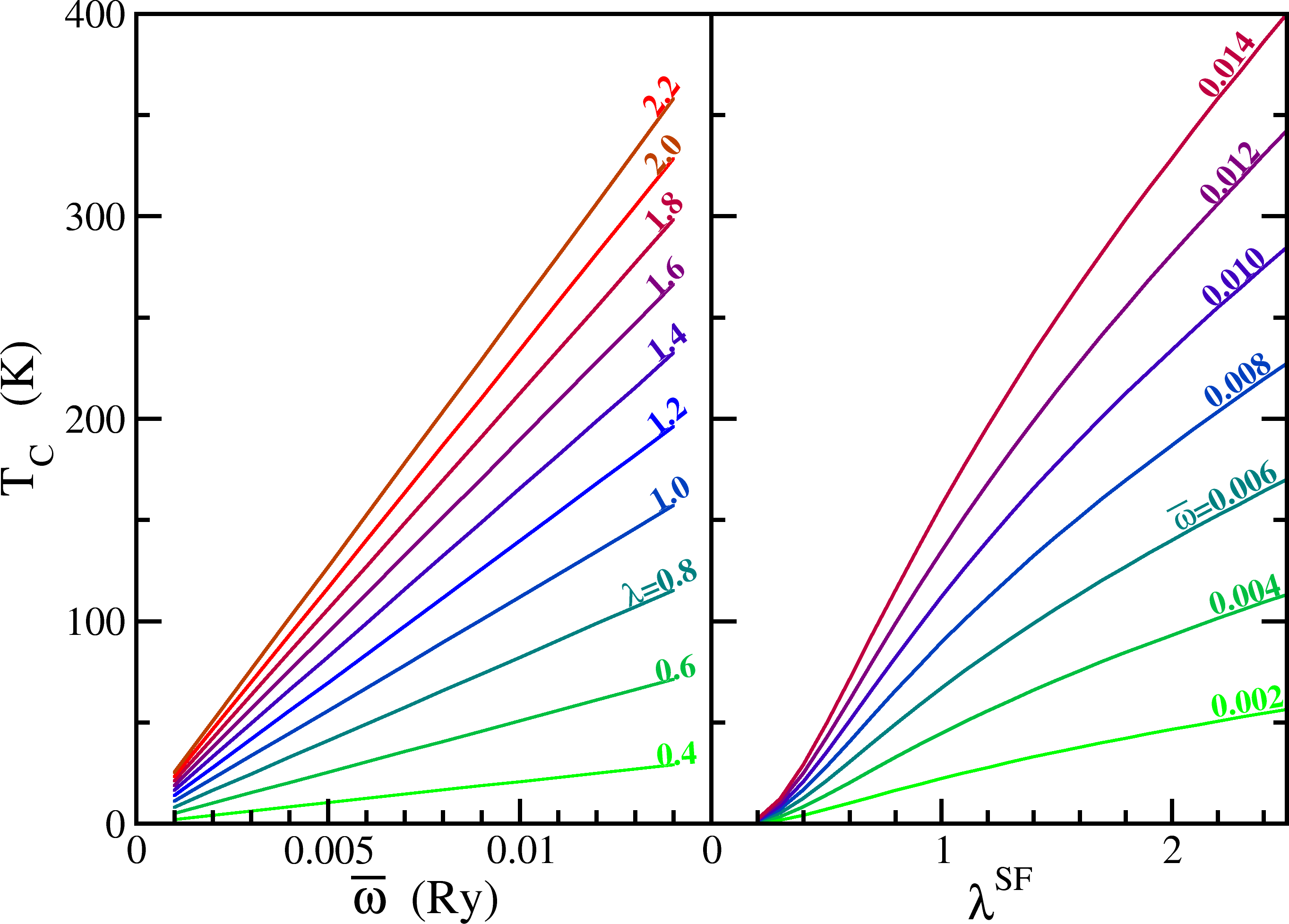
Refer to caption — Figure 1: (left) $T_{\text{c}}$ for different $\lambda^{{\scriptscriptstyle\text{SF}}}$ as a function of the average $\bar{\omega}$ . (right) Analogous plot, here for several $\bar{\omega}$ as a function of $\lambda^{{\scriptscriptstyle\text{SF}}}$ .

We modify the SF by acting on the parameters $\bar{\omega}$ and $\lambda_{{\scriptscriptstyle IJ}}^{{\scriptscriptstyle\text{SF}}}$ . In Fig. 1 we show the critical temperature as a function of $\bar{\omega}$ and $\lambda_{{\scriptscriptstyle IJ}}^{{\scriptscriptstyle\text{SF}}}$ . From Eliashberg theory for phonon driven superconductors we have knowledge of the following relations between characteristic frequency and average coupling strength[59, 60]:

	$\displaystyle T_{\text{c}}$	$\displaystyle\propto\bar{\omega}\,\mathrm{e}^{-\alpha/\lambda}\text{ for small }\lambda$		(39)
	$\displaystyle T_{\text{c}}$	$\displaystyle\propto\bar{\omega}\,\sqrt{\lambda}\text{ for large }\lambda.$		(40)

On the right hand side of Fig. 1 we can recognize the exponential and square root behavior with respect to $\lambda^{{\scriptscriptstyle\text{SF}}}$ . The transition between small and large coupling takes place at $\lambda^{{\scriptscriptstyle\text{SF}}}\sim 1.5$ for $\bar{\omega}=0.15$ Ryd. For the dependence of $T_{\text{c }}$ with respect to $\bar{\omega}$ , we find a linear behavior.

This result is not accidental, because the sign change of the gap leads effectively to an attractive interaction between the two bands, therefore within this simplified model there is no formal difference between spin-fluctuation repulsive pairing and conventional phononic attraction.

Within such a model calculation we can estimate the coupling strength in the iron based superconductors, simply by the experimental knowledge that the characteristic energy of the magnetic fluctuations are of about $20\text{ meV}$ [5]. This implies a coupling $\lambda^{{\scriptscriptstyle\text{SF}}}$ of about 1 (neglecting phononic and Coulomb effects) to reach the critical temperatures of $\sim 10\text{ K}$ found in these compounds.

VI.3 Interplay between Coulomb, Spin-Fluctuation and Phonon Contribution

In the previous section we have observed that the features of the SCDFT gap equation with a SF interaction is relatively simple and similar to the conventional phononic case. Here we add the effect of phonon and Coulomb interactions. This will create a frustration on the SC potential because the three interaction will compete against each other.

We use the same spin-fluctuation spectrum in Eq. (38) and fix $\lambda^{{\scriptscriptstyle\text{SF}}}=1.2$ and $\bar{\omega}=0.01\text{ Ryd}$ . The Coulomb interaction is very different in nature, compared to the SF. In particular its frequency dependence develops in the plasmonic energy scale (eV). We therefore ignore it, and assume a flat interaction with respect to $\omega$ .

It is expected, that this interaction decays like $\frac{1}{\boldsymbol{q}^{2}+\boldsymbol{q}_{\text{TF}}^{2}}$ , where $\boldsymbol{q}_{\text{TF}}$ is the Thomas-Fermi screening vector. Therefore the contribution for small momentum transfer (intra-band) should be much larger than the inter-band contribution corresponding to $\boldsymbol{q}_{\text{c}}\approx\boldsymbol{k}-\boldsymbol{k}^{\prime}$ . Similarly for scattering from the Fermi level to high-energy states, the scattering should become momentum independent[61]. We model this picture in the following way:

w_{{\scriptscriptstyle IJ}}\left(E_{1},\!E_{2}\right)=\begin{cases}N_{{\scriptscriptstyle J}}\left(E_{2}\right)\left(U_{0}+U_{1}\mathrm{e}^{-\kappa\left(E_{1}^{2}+E{}_{2}^{2}\right)}\right)\\ \text{if }I=J\\ \\ N_{{\scriptscriptstyle J}}\left(E_{2}\right)U_{0}\\ \text{if }I\neq J.\end{cases}

(41)

The diagonal part $w_{{\scriptscriptstyle II}}\left(E_{1},\!E_{1}\right)$ of this interaction is shown in Fig. 2. For the parameters of the Coulomb interaction we choose $N_{{\scriptscriptstyle J}}\left(\epsilon_{{\scriptscriptstyle\text{F}}}\right)U_{0}=0.2,$ $U_{1}=\frac{U_{0}}{2}$ . The parameter $\kappa$ is used to control the Coulomb interaction: If $\kappa$ is large the Coulomb interaction decays very quickly in energy.

Due to the choice of an electron hole symmetric DOS ( $N_{+}\left(E\right)=N_{-}\left(E\right)$ ) and interaction, the gap function is also totally symmetric: $\varDelta_{{\scriptscriptstyle I}}\left(E\right)=\varDelta_{{\scriptscriptstyle I}}\left(-E\right)$ and $\varDelta_{+}\left(E\right)=-\varDelta_{-}\left(E\right)$ and hence only the positive branch $\varDelta_{+}\left(E\right)$ is shown in Fig. 2. Note that within this symmetry a constant coulomb interaction ( $\kappa\to\infty$ ) cancels out completely from the gap equation 36.

In general the gap function shows a typical form, being constant close to the Fermi level, followed by an extremum and a decay for larger energies [62, 18]. By decreasing the value of $\kappa$ the Coulomb contribution starts to influence the results. The critical temperature decreases, due to repulsion within one band and the gap starts to show dips. The dips indicate the regime, where the Coulomb interaction competes with the spin-fluctuation. For $\kappa<1$ the Coulomb contribution are strong enough to flip the sign of the gap function for certain energies. The sign change of the gap function at higher energies reduces the effect related to the repulsive Coulomb term in the gap equation 36.

Effectively, the Coulomb contribution on the full energy scale may be mapped to a reduced effective Coulomb term on a smaller energy scale due to the sign change of the gap function. Hence, the sign change of the gap function is the way Coulomb renormalization happens in SCDFT[18, 61]. Note that the sign change of the gap happens far away from the Fermi level.

However, for $\kappa=4$ the Coulomb contribution still decays faster in energy than the spin-fluctuation term, which leads to one more sign change in the large energy regime (dash-dotted blue line in Fig. 2). If we decrease the $\kappa$ further the Coulomb contribution dominate also in the large energy range and the gap changes sign only once.

Note, that the critical temperature converges quickly with respect to $\kappa.$ This indicates, that the Coulomb interaction influences the critical temperature only in a small energy window for the symmetric two band system and the renormalization of the gap is not effecting the critical temperature strongly.

To verify this observation, we test different densities of states instead of the constant one used so far: The different functions are step and square root functions which represent a two and three dimensional system, respectively and a Gaussian peak. The different functions are shown in Fig. 3. The non flat functions cut away the long energy tails of the gap function. However, the effect on the critical temperature is rather small.

What has a strong effect on $T_{\text{c}}$ is a change of the ratio $\frac{N_{+}\left(\epsilon_{\text{F}}\right)}{N_{-}\left(\epsilon_{\text{F}}\right)}=1$ (magenta line in Fig. 2). This verifies that in the two band system with a sign changing gap, only a small energy region around the Fermi level matters for the Coulomb repulsion. This is very different from the one band case, where the Coulomb renormalization at large energies is an essential effect.

Last we consider the inclusion of the purely attractive phonon contribution. It’s behavior is rather straightforward. If a single phonon peak is included ( Eq. 38 ) providing the same coupling between all bands, the critical temperature reduces by increasing $\lambda^{{\scriptscriptstyle\text{Ph}}}$ . Until a the phononic coupling strength reaches the value of $\lambda^{{\scriptscriptstyle\text{SF}}}$ . The phonons dominate the gap equation and the symmetry of the gap changes. The $s_{\pm}$ state favored by the repulsive interactions is suppressed and an $s_{++}$ state is found. From this point the $T_{\text{c}}$ starts to rise again with increasing $\lambda^{{\scriptscriptstyle\text{Ph}}}$ .

VII Summary and Outlook

In this work we have derived a fully ab-initio effective electron-electron interaction containing the effect of a pairing mediated by spin-fluctuation. The derivation starts from many-body perturbation theory and the introduction of a self-energy function, containing the relevant diagrams originating from its vertex part, therefore going beyond the $GW$ approximation. The vertex correction enter the expression in the form of the particle-hole propagator, which is a highly non-local object determined by a BSE. The solution of the BSE would be computationally not feasible for realistic systems instead, in Sec. III.3, we propose a local approximation for the particle-hole propagator. In this limit the equation for the self-energy becomes very transparent: spin-fluctuations enter via the magnetic response functions, that can be calculated effectively[63, 58] within linear response TD-DFT, and the coupling to the electrons is mediated by the exchange-correlation kernel.

This effective interaction is in principle applicable to any theory of SC, however in this work we cast it into the framework of SCDFT by the construction of an explicit xc kernel (Sec. V). In this way the full gap equation remains completely parameter free.

We show a first application of the new functional (Sec. VI) to a two band electron gas model. Application to real materials will follow, however this further step needs the calculation of the magnetic response function for the real system and will be the subject to further investigation.

References

[1] J. Bednorz and K. Müller, Zeitschrift für Physik B Condensed Matter 64, 189 (1986).
[2] J. G. Bednorz and K. A. Müller, Rev. Mod. Phys. 60, 585 (1988).
[3] Y. Kamihara, H. Hiramatsu, M. Hirano, R. Kawamura, H. Yanagi, T. Kamiya, and H. Hosono, Journal of the American Chemical Society 128, 10012 (2006).
[4] P. Hirschfeld, M. Korshunov, and I. Mazin, Rep. Prog. Phys. 74, 124508 (2011).
[5] G. R. Stewart, Rev. Mod. Phys. 83, 1589 (2011).
[6] D. Manske, Theory of Unconventional Superconductors, Cooper-Pairing Mediated by Spin Excitations (Springer-Verlag Berlin Heidelberg, 2004).
[7] T. Saito, S. Onari, and H. Kontani, Phys. Rev. B 82, 144510 (2010).
[8] P. A. Lee, N. Nagaosa, and X.-G. Wen, Rev. Mod. Phys. 78, 17 (2006).
[9] L. N. Oliveira, E. K. U. Gross, and W. Kohn, Phys. Rev. Lett. 60, 2430 (1988).
[10] M. Lüders, M. A. L. Marques, N. N. Lathiotakis, A. Floris, G. Profeta, L. Fast, A. Continenza, S. Massidda, and E. K. U. Gross, Phys. Rev. B 72, 024545 (2005).
[11] A. Sanna and E. K. U. Gross, To be pubblished .
[12] A. Floris, G. Profeta, N. N. Lathiotakis, M. Lüders, M. A. L. Marques, C. Franchini, E. K. U. Gross, A. Continenza, and S. Massidda, Phys. Rev. Lett. 94, 037004 (2005).
[13] G. Profeta, C. Franchini, N. N. Lathiotakis, A. Floris, A. Sanna, M. A. L. Marques, M. Lüders, S. Massidda, E. K. U. Gross, and A. Continenza, Phys. Rev. Lett. 96, 047003 (2006).
[14] A. Sanna, G. Profeta, A. Floris, A. Marini, E. K. U. Gross, and S. Massidda, Phys. Rev. B 75, 020511 (2007).
[15] A. Floris, A. Sanna, S. Massidda, and E. K. U. Gross, Phys. Rev. B 75, 054508 (2007).
[16] P. Cudazzo, G. Profeta, A. Sanna, A. Floris, A. Continenza, S. Massidda, and E. K. U. Gross, Phys. Rev. Lett. 100, 257001 (2008).
[17] P. Cudazzo, G. Profeta, A. Sanna, A. Floris, A. Continenza, S. Massidda, and E. K. U. Gross, Phys. Rev. B 81, 134506 (2010).
[18] M. A. L. Marques, M. Lüders, N. N. Lathiotakis, G. Profeta, A. Floris, L. Fast, A. Continenza, E. K. U. Gross, and S. Massidda, Phys. Rev. B 72, 024546 (2005).
[19] R. Akashi and R. Arita, Phys. Rev. Lett. 111, 057006 (2013).
[20] C. Bersier, A. Floris, A. Sanna, G. Profeta, A. Continenza, E. K. U. Gross, and S. Massidda, Phys. Rev. B 79, 104503 (2009a).
[21] A. Sanna, C. Franchini, A. Floris, G. Profeta, N. N. Lathiotakis, M. Lüders, M. A. L. Marques, E. K. U. Gross, A. Continenza, and S. Massidda, Phys. Rev. B 73, 144512 (2006).
[22] L. Boeri, O. V. Dolgov, and A. A. Golubov, Phys. Rev. Lett. 101, 026403 (2008).
[23] P. Morel and P. W. Anderson, Phys. Rev. 125, 1263 (1962).
[24] I. I. Mazin, D. J. Singh, M. D. Johannes, and M. H. Du, Phys. Rev. Lett. 101, 057003 (2008).
[25] P. Hohenberg and W. Kohn, Phys. Rev. 136, B864 (1964).
[26] T. Kreibich, R. van Leeuwen, and E. K. U. Gross, Phys. Rev. A 78, 022501 (2008).
[27] Y. Nambu, Phys. Rev. 117, 648 (1960).
[28] C. A. Kukkonen and A. W. Overhauser, Phys. Rev. B 20, 550 (1979).
[29] E. K. U. Gross and S. Kurth, International Journal of Quantum Chemistry 40, 289 (1991).
[30] J. Bardeen, L. N. Cooper, and J. R. Schrieffer, Phys. Rev. 108, 1175 (1957).
[31] R. S. Gonnelli, D. Daghero, D. Delaude, M. Tortello, G. A. Ummarino, V. A. Stepanov, J. S. Kim, R. K. Kremer, A. Sanna, G. Profeta, and S. Massidda, Phys. Rev. Lett. 100, 207004 (2008).
[32] C. Bersier, A. Floris, P. Cudazzo, G. Profeta, A. Sanna, F. Bernardini, M. Monni, S. Pittalis, S. Sharma, H. Glawe, A. Continenza, S. Massidda, and E. K. U. Gross, Journal of Physics: Condensed Matter 21, 164209 (2009b).
[33] C. C. Tsuei and J. R. Kirtley, Rev. Mod. Phys. 72, 969 (2000).
[34] L. Hedin, Phys. Rev. 139, A796 (1965).
[35] A. Migdal, J. Exptl. Theoret. Phys (U.S.S.R.) 34, 996 (1958).
[36] T. A. Maier, S. Graser, D. J. Scalapino, and P. Hirschfeld, Phys. Rev. B 79, 134520 (2009).
[37] J. Wen, G. Xu, Z. Xu, Z. W. Lin, Q. Li, Y. Chen, S. Chi, G. Gu, and J. M. Tranquada, Phys. Rev. B 81, 100513 (2010).
[38] S. M. Shapiro, G. Shirane, and J. D. Axe, Phys. Rev. B 12, 4899 (1975).
[39] R. E. Prange, Phys. Rev. 129, 2495 (1963).
[40] A more general and unbiased way would be to start from Hedin cycle[34] and iterate it self-consistently. This would lead also include the $T$ -matrix diagrams considered here, but at a slow convergence rate[34].
[41] E. Sasioglu, A. Schindlmayr, C. Friedrich, F. Freimuth, and S. Blügel, Phys. Rev. B 81, 054434 (2010).
[42] G. Onida, L. Reining, and A. Rubio, Rev. Mod. Phys. 74, 601 (2002).
[43] E. E. Salpeter and H. A. Bethe, Phys. Rev. 84, 1232 (1951).
[44] J. Hertz and D. Edwards, Journal of Phys. F: Metal Physics 3, 2174 (1973).
[45] S. Doniach and S. Engelsberg, Phys. Rev. Lett. 17, 750 (1966).
[46] V. P. Zhukov, E. V. Chulkov, and P. M. Echenique, Phys. Rev. B 72, 155109 (2005).
[47] P. Romaniello, F. Bechstedt, and L. Reining, Phys. Rev. B 85, 155131 (2012).
[48] G. Vignale and K. S. Singwi, Phys. Rev. B 32, 2156 (1985).
[49] L. G. Molinari, Phys. Rev. B 71, 113102 (2005).
[50] F. Aryasetiawan and S. Biermann, Phys. Rev. Lett. 100, 116402 (2008).
[51] N. F. Berk and J. R. Schrieffer, Phys. Rev. Lett. 17, 433 (1966).
[52] L. J. Sham and W. Kohn, Phys. Rev. 145, 561 (1966).
[53] R. Del Sole, L. Reining, and R. W. Godby, Phys. Rev. B 49, 8024 (1994).
[54] E. Runge and E. K. U. Gross, Phys. Rev. Lett. 52, 997 (1984).
[55] I. Mazin, Nature 464, 183 (2010).
[56] L. J. Sham and M. Schlüter, Phys. Rev. Lett. 51, 1888 (1983).
[57] M. Marques Ph.D. thesis, Density Functional Theory for Superconductors, Exchange and Correlation Potentials for Inhomogeneous Systems (Bayerische Julius-Maximilians Universität Würzburg, 1998).
[58] F. Essenberger, P. Buczek, A. Ernst, L. Sandratskii, and E. K. U. Gross, Phys. Rev. B 86, 060412 (2012).
[59] W. L. McMillan, Phys. Rev. 167, 331 (1968).
[60] P. B. Allen and R. C. Dynes, Phys. Rev. B 12, 905 (1975).
[61] S. Massidda, F. Bernardini, C. Bersier, A. Continenza, P. Cudazzo, A. Floris, H. Glawe, M. Monni, S. Pittalis, G. Profeta, A. Sanna, S. Sharma, and E. K. U. Gross, Superconductor Science and Technology 22, 034006 (2009).
[62] A. Sanna Ph.D. thesis, Application of Density Functional Theory for Superconductors to real materials (Universitià degli Studi di Cagliari, 2007).
[63] P. Buczek, A. Ernst, P. Bruno, and L. M. Sandratskii, Phys. Rev. Lett. 102, 247206 (2009).