Non-contractible loops in the dense loop model on the cylinder
Abstract
A lattice model of critical dense polymers is considered for the finite cylinder geometry. Due to the presence of non-contractible loops with a fixed fugacity , the model at is a generalization of the critical dense polymers solved by Pearce, Rasmussen and Villani. We found the free energy for any height and circumference of the cylinder. The density of non-contractible loops is obtained for and large . The results are compared with those found for the anisotropic quantum chain with twisted boundary conditions. Using the latter method we derived for any model and an arbitrary fugacity.
pacs
05.40.-a, 02.50.Ey, 82.20.-wKeywords: dense polymers, free fermion model, spanning graphs, XXZ chain, Temperley-Lieb algebra.
I Introduction
The dense loop model [1] is defined by drawing two arcs in each elementary cell of the square lattice: the two possible states of the cell are shown in Fig. 1. The lines on the whole lattice with appropriate boundary conditions form a system of closed loops with the Boltzmann weight ascribed to every loop.


Two particular cases, and are of special interest. At , the model can be mapped to the bond percolation problem, the six vertex model and the quantum chain [2, 3]. At , the bulk loops disappear and the set of lines is converted into the model of critical dense polymers [4]. This model is a recent representative of the more general two-dimensional polymer theory initiated by Saleur and Duplantier in the context of a conformal field theory [5, 6, 7]. The dense polymer model is the first member of the Yang-Baxter integrable series of logarithmic minimal models. In the scaling limit, the central charge is and the conformal weights yield the Kac formula for the infinitely extended Kac table [4].
Pearce, Rasmussen and Villani [8] have solved the dense polymer model on a cylinder using the single-row transfer matrix and the inverse identity for the transfer matrix. They solved the inverse identity for different boundary conditions, including the case in which noncontractible loops are allowed. The structure of the inversion identity dictates its solvability at fugacity 2 of the non-contractible loops. The fixed fugacity prevents the evaluation of the free energy as a function of fugacity, so the average number of loops on the cylinder remains unknown. At the same time, the statistics of noncontractible loops is important as it is related to the conformal properties of the model in the continuous limit. The standard tool for determination of the central charge of a conformal field theory, corresponding to a given lattice model at the critical point, is the expansion of the free energy of an infinitely long cylinder of finite perimeter . The two leading terms of the expansion have the form
| (1) |
where is the bulk density of the free energy per unit length, and is an effective central charge, which is a combination of the true central charge and a correction term depending on the boundary conditions [9]. It will be shown below, that the contribution of the non-contractible loops in is of the order of . Therefore depends on the presence of such loops and their fugacity in the case of two-dimensional lattice models, and on a twist parameter in the corresponding quantum chains.
In this paper, we solve the model of dense polymers on the cylinder by calculating the partition function of a spanning web model on a finite cylinder in the presence of cycles winding around the cylinder. Our aim is to evaluate the grand partition function of the dense polymers model at arbitrary fugacity of the non-contractible loops and to find their density per unit height of the cylinder.
For an infinite cylinder of perimeter , there is an alternative, albeit simpler, method to compute the free energy and the density of the non-contractible loops for any model at arbitrary fugacity. The states of the model can be defined in terms of a connectivity condition for the points of intersection between the loops and a horizontal line cutting the loops at these points. Two points are connected by a link if there exists a line between them via the half space above the cut. For instance, imposing periodic boundary conditions in horizontal direction on the lattice in Fig. 2 and specifying the boundary conditions at the upper edge, we obtain three minimal links between points 1 and 6, 2 and 3, 4 and 5, which are points of intersection between loops and the bottom line of the lattice belonging to the upper half-plane. A typical configuration of links for a larger lattice is given in Fig. 3.

The link representation allows definitions of the transfer matrix and the Hamiltonian as elements of the periodic Temperley-Lieb algebra [10, 11]. The same algebra has a matrix representation that takes us to the spin- quantum chain with a twist depending on the fugacity. The ground-state energy is known analytically [13] for large values of for any anisotropy related to the parameter of the model. The Temperley-Lieb algebra has a quotient with a free parameter that can be identified with the fugacity of noncontractible loops, so we can compute their density from the ground state of the Hamiltonian. In the special case of , one can use a Jordan-Wigner transformation and obtain the ground state energy for any finite explicitly.
The paper is organized as follows. In Section II, we present the calculation of the density of noncontractible loops using the quantum chain. We start with this presentation since, unlike the lattice case, the calculation is almost trivial. We also show that the probability distribution of noncontractible loops is not Gaussian. In Section III, we consider the special case . Due to the absence of contractible loops, the loop model can be mapped on the spanning webs model. In the latter model, one can generalize the Kirchhoff theorem and bring the calculation to that of determinants. The details of the proof are given in the Appendix. The calculation of the partition function on a torus is presented in Section IV, and the result is given by Eq. (31). The case of finite cylinders of height and perimeter , with different boundary conditions on the top and bottom of the cylinder, is briefly mentioned in Section V. Finally, in Section VI, we consider the case of an infinite cylinder by taking to infinity, and we compare the thus obtained results for the density of the noncontractible loops to those of Section II.
II The density of noncontractible loops obtained from the XXZ quantum chain
We remind the reader of a few facts about the periodic Temperley-Lieb algebra (PTL) and some of its representations [11]. This algebra provides the key to the calculation of the density of non-contractible loops. The PTL has generators () satisfying the relations
| (2) |
where is a parameter.
We are going to consider the -even case only. The PTL is infinite-dimensional therefore we take a quotient which makes it finite dimensional:
| (3) |
where
| (4) |
We are interested in two representations of the PTL with the quotient (3). The first one is the spin representation, in which
| (5) |
where
| (6) |
and are the Pauli matrices [10], and is the boundary twist parameter.
In the second representation, the generators act in the vector space of periodic link patterns. Each link pattern is one of the configurations of nonintersecting arches joining sites on a circle. One can visualize the circle on a cylinder. Besides the link patterns on the same cylinder, one takes circles with no sites on them to represent noncontractible loops. In Fig. 4 we show the six configurations for and .

With few exceptions, the generators act on the configurations in the standard way (as in the non-periodic Temperley-Lieb algebra) [12]. In Fig. 5, one sees the action of the generator on one of the configurations of Fig. 4. The factor appears due to a contractible loop. The exceptions occur if one considers configurations having an arch of the size of the system and if the generator acts on the bond between the ends of the arch, see Fig. 6(a). The action of on the third configuration of Fig. 4 produces a new circle and one gets a configuration with . Instead of considering configurations with various numbers of noncontractible loops, we are going to consider configurations with no noncontractible loops but, as a result of the action of , we multiply by fugacity instead of adding a noncontractible loop; see Fig. 6(b). With this rule, one obtains a representation of the PTL with the quotient (3), and relates to the fugacity of noncontractible loops.


We consider the Hamiltonian
| (7) |
Using the representation in terms of link paths of the PTL, this Hamiltonian is equal up to a factor to the Hamiltonian obtained from the transfer matrix of the models [8]. This factor is equal to the sound velocity :
| (8) |
In the spin representation of the PTL, using a similarity transformation, the Hamiltonian can be written as
| (9) |
This Hamiltonian which is the quantum chain with a twist is integrable and its ground-state and energy spectrum is known [13]. In particular, the ground-state energy is
| (10) |
where is the bulk energy density. Notice that the choice () and used in Ref. [8] corresponds to the model. From (10) one can get two quantities of interest. Firstly, taking into account that the density of the spin current is
| (11) |
its average value at large values of is, see Eqs. (5) and (7)),
| (12) |
Since the coefficient in Eq. (12) is dimensionless, we expect it to be universal. A second quantity of interest is the density of noncontractible loops:
| (13) |
Notice that the density of noncontractible loops is proportional to the current density (a physical explanation of this observation is still missing). We observe also that the dependence on in has a very simple form.
There is a simple way to check if the probability distribution of noncontractible loops is Gaussian or not. Using Eqs. (6) and (10) one can can compute all the moments of the probability distribution. They are all of order . One can check that, for example, the identity
| (14) |
valid for a Gauss distribution, is not satisfied.
Using the relation (6), one obtains for (, no contractible loops)
| (15) |
and
| (16) |
Expressions (15) (16) are going to be compared to those obtained from spanning webs model presented in the next sections.
For the same case () only, one has a simple expression for the ground state energy valid for any value of :
| (17) |
Using this relation, one can compute the density of noncontractible loops for any fugacity and any size of the system .
III The spanning webs model on the rotated square lattice
Another representation of the model relates loop configurations to clusters of bonds on sublattices of the original lattice. The square lattice of sites with integer coordinates can be divided into two sublattices, black and white. For sites of the black sublattice the sum of coordinates is even, while for sites of the white one it is odd. The bijection between loop and bond configurations is shown in Fig. 7. The neighboring sites of each sublattice are connected by a bond if it does not intersect the borderlines of the elementary cell. Each connected cluster of bonds in the bulk of the lattice is situated inside a loop. Each bulk cluster on the black sublattice is surrounded by a connected cluster of bonds on the white sublattice and vice versa.


At , the absence of bulk loops contractible to a point implies the absence of isolated clusters of bonds on the black or white sublattice. The allowed bond configurations are the so called spanning webs, i.e., the graphs containing all vertices of a sublattice, noncontractible loops arising from the periodic boundary conditions and spanning trees connected either to open boundaries or to the noncontractible loops. Clearly, due to the bijection between bonds and elementary cells, the presence of every noncontractible loop in the bulk of the cylinder is equivalent to the presence of a pair of noncontractible polymers in the dense polymer representation. If there are no noncontractible loops in the system, polymers can propagate from the top to the bottom of the cylinder. These polymers are treated as defect lines that separate clusters of bonds one from another.
The reformulation of the dense polymer model in terms of bond configurations leads us to the standard problem of spanning graphs on the square lattice. The cycle-free spanning graphs are called spanning trees; the graphs containing a number of cycles are called spanning webs. The enumeration of spanning trees is traced back to the classical Kirchhoff theorem [14, 19]. The spanning web model appears in statistical mechanics as the Temperley representation [15] of the dimer model solved by Kasteleyn [16] and by Temperley and Fisher [17]. A particular case we consider here is the spanning web model on a cylinder with noncontractible cycles supplied by fugacity . This decoration needs a generalization of the Kirchhoff theorem. A similar model, considered as the (1,2) logarithmic minimal model, has been solved in [18], where the fugacity of noncontractible loops was first introduced. A basic accent of the present work is the calculation of the density of noncontractible cycles in a finite geometry.
We consider an oriented labeled graph with vertex set and set of bonds . Vertices are the sites of a finite square lattice rotated by and wrapped on a cylinder. The graph can be considered as a sublattice of square superlattice with standard orientation, containing rows and columns of cells. Vertices of the superlattice are shown in Fig. 9 as open and filled circles. The vertex set is the sublattice of filled circles.

For convenience, in the remainder we call the “height” and the “perimeter” of the cylinder. Let the cells of be labeled by the integer coordinates and , so that the row is the bottom boundary of the cylinder and the row is its top boundary. For the sake of convenience, both and are chosen to be even. The vertex set of the rotated square lattice then consists of the vertices of the sublattice of with, say, an even sum of the horizontal and vertical coordinates, i.e., . Explicitly, we have
| (18) |
The edges in we take oriented from a site to its nearest neighbors on the right-hand side, and . We call this direction “positive”, and the opposite one, from a site to its nearest neighbors on the left-hand side, and , we call “negative”.
We find it convenient to analyze the construction of spanning web configurations on the above oriented graph by using the arrow representation; see, e.g., [19]. Accordingly, to each vertex we attach an arrow directed along one of the bonds incident to it. Each arrow defines a directed bond and each configuration of arrows on defines a spanning directed graph (digraph) with set of bonds depending on .
A cycle of length is a sequence of directed bonds ,, , where all , are distinct. If both and belong to the same spanning web we say that it contains a cycle of length 2. Our aim is to study sets of spanning digraphs with no other cycles than those which wrap the cylinder. The relevant configurations will be enumerated with the aid of a generating function defined as the determinant of an appropriately constructed weight matrix:
| (19) |
In this respect, the derivation of the above relationship, see the Appendix, is merely a generalization of the matrix Kirchhoff theorem [14].
The elements , of the matrix , associated with the graph , are explicitly given as
| (20) |
Here is the order of vertex in , , and the condition “ is a right (left) neighbor of ” means that if , then []. Note that all closed paths which do not wrap the cylinder contain an equal number of edges with either orientations, hence their weight in remains the same as in . Therefore, all the configurations that contain such closed paths (contractible cycles) cancel out in the expansion of . On the other hand, cycles generated by off-diagonal elements that wrap the cylinder change their sign, because they contain edges oriented in one direction exceeding by the number of edges in the opposite direction. This amounts to the total factor of or depending on the orientation. Therefore, each noncontractible cycle with a given orientation is counted twice, however, with different weight — once it enters into the determinant expansion with the unit weight, being generated by diagonal elements of the matrix , and second time it enters with a factor or (depending on the orientation) as generated by off-diagonal elements of that matrix. Thus, the total number of noncontractible cycles, irrespective of their origin and orientation, is given by the coefficient in front of the corresponding power of in the series expansion of the partition function. In general, besides the noncontractible cycles, the average number of which is controlled by fugacity , the spanning digraph contains tree subgraphs connected to the cycles. All branches of the trees can be generated only by the diagonal elements of and, hence, carry unit weight.
IV The partition function on a torus
To calculate the generating function in expression (19), we make some initial transformations that allow us to easily diagonalize the matrix . First of all, the decomposition (18) of the vertex set of the rotated square lattice suggests its rearrangement by combining all pairs of nearest neighbors and , , into two-site unit cells. Thus we obtain a square array of unit cells with the connectivity of a triangular lattice. Under neglect of the boundary effects at the top and bottom of the cylinder, we describe the weighted connectivity of the sites in a unit cell with their neighbors in , taking into account the bond orientation, by introducing the following matrices:
Now the matrix , see Eq. (20), can be written as
| (21) |
Here is the matrix
| (22) |
and is the matrix transposed of . Now we note that both and are diagonalized by the similarity transformation
where the is the matrix with elements
| (23) |
Since , we have
Therefore, with the similarity transformation generated by the matrix we can diagonalize the matrix in the and - dimensional subspaces. Then for the determinant we readily obtain
| (24) |
where is the matrix,
| (25) |
It is convenient to cast its determinant in the form
| (26) |
where . Thus, from Eq. (24) we obtain the -dependent part of the partition function
| (27) |
Next we set
| (28) |
where
| (29) |
Now, making use of the identity
| (30) |
with , we perform exactly the product over :
| (31) |
Strictly speaking, this expression is valid for spanning webs on a torus, since we have not considered boundary conditions at the edges of the cylinder properly. For the sake of completeness, in the next section we present the exact expressions for the partition function under closed and open boundary conditions at the top and bottom of a finite-size cylinder.
V Cylindrical boundary conditions
In the preceding section we computed the partition function of the spanning webs without contractible loops on the torus. Here we consider the cases when the boundaries at the top and bottom of cylinder are closed or open; see Fig.(10). It can be seen from the figure that there is a difference between the cases of odd and even : in the latter case, the lower edge is shifted with respect to the top one. In our considerations is even, whereas is of any parity.

In the case of both boundaries open, the diagonal elements of the matrix (20)are , because every vertex has four outgoing edges. The partition function is, compare to (27),
| (32) |
The partition functions in the case of all the other uniform boundary conditions can be expressed in terms of as follows:
In the case of both closed boundary conditions,
| (33) |
in the case mixed open-closed boundary conditions,
| (34) |
and for the torus
| (35) |
From these expressions, it can be easily seen that the density of noncontractible loops, see the next section, is equal for different boundary conditions in the limit .
VI Density of non-contractible loops
The average density (per unit height of the cylinder) of the noncontractible cycles as a function of the fugacity is defined as
| (36) |
Since we are interested in the case of the density on an infinitely long cylinder, we expect the boundary corrections to vanish in the limit . To take this limit, we factor out another -independent term from ,
| (37) | |||||
and make use of the density definition (36):
| (38) |
Hence, in the limit
| (39) | |||||
where ( is even)
| (40) |
Therefore, when , the essential contribution in comes from the integration over the two small intervals and with . To leading-order in , it suffices to take the linear term in the expansion
| (41) |
which yields
| (42) | |||||
Extending the lower limit in the latter integral to , we finally obtain the general expression
| (43) |
We are going to compare the obtained result with Eq. (15) in the interval of the loop fugacity corresponding to real values of the twist parameter . Toward that end, we transform the bottom expression in Eq.(43),
| (44) |
and remember that each cycle in the spanning web model corresponds to a pair of non-contractible loops with fugacity . Then, the density of non-contractible loops in the dense polymer model is
| (45) |
in full agreement with (15).
For and , we use the formula
| (46) |
and get
| (47) |
We see that the formula for corresponds to the quantum chain result (16) with the complex twist
| (48) |
The crucial check of Eq.(45) is the value of density for , when the fugacity of noncontractible cycles in the spanning web model is . In this case, the noncontractible cycles enter into the partition function as two nonweighted sequences of bonds oriented clockwise and anticlockwise. Due to symmetry of the model, the spread of each sequence in the horizontal direction (that is, by the definition of loops) coincides in average with that in the direction of the cylinder axis. Each two loops on the rotated lattice (Fig.9) are separated by a loop on the dual lattice. Thus, the spanning web configuration in the vertical direction is a sequence of sandwiches of loops and dual loops of average thickness . Then, the density of web cycles is and the density of noncontractible loops is .
We note that Morin-Duchesne et al. [20] have obtained the inversion relation for any which should allow one to obtain our results in a different way.
Acknowledgments
We thank P. Pearce for helpful discussions. This work was supported by RFBR Grant No 12-01-00242a, the Heisenberg-Landau program, the DFG grant No. RI 317/16-1 and the Brazilian agencies FAPESP and CNPq.
Appendix
In this Appendix, we give a detailed derivation of the expression (19) for the generating function of all spanning digraphs on which have no contractible cycles. We begin with an examination of the determinant expansion of the usual Laplace matrix for the graph . Let the vertices be labeled in arbitrary order from 1 to . Then has the following elements ()
| (49) |
where is the order of vertex in the rotated square lattice . Since the matrix has a zero eigenvalue, its determinant vanishes. On the other hand, the Leibnitz formula expresses the determinant of as a sum over all permutations of the set :
| (50) |
where is the symmetric group and is the signature of the permutation . The identity permutation in Eq. (50) yields the term equal to the number of all possible arrow configurations on .
In general, each permutation can be factored into a product (composition) of disjoint cyclic permutations, say . This representation partitions the set of vertices into non-empty disjoint subsets — the orbits of the corresponding cycles , . More precisely, if is the orbit of , then and , where is the cardinality of the orbit , or equivalently, the length of the cycle . The orbits consisting of just one element, if any, constitute the set of fixed points of the permutation: . In the case of the identity permutation , all orbits consist of exactly one element, , , and . A cycle of length will be called a proper cycle. A proper cycle of length 2 corresponds to two oppositely directed edges that connect a pair of adjacent vertices: , . Note that the vertices of an orbit of cardinality are connected by a closed path on which can be traversed in two opposite directions: if is the cycle defined by , then the reverse cycle can be represented as .
Now we take into account that the proper cycles on are of even length only, hence the signature of every permutation in the expansion of the determinant depends on the number of proper cycles in its factorization, i.e., if , where , , then . Thus, the terms in Eq. (50) can be rearranged according to the number of disjoint proper cycles as follows:
| (51) |
Here is the -fold composition of the cyclic permutation of even length , , so that and . Note that all nonvanishing off-diagonal elements are equal to .
The above expansion reveals the following features: (i) As expected, all spanning digraphs on have at least one proper cycle; (ii) Each term with represents a set of distinct spanning digraphs, which have in common the specified cycles , and they differ in the oriented edges outgoing from the vertices . These oriented edges may form cycles on their own which do not enter into the list ; (iii) Since the sets and are disjoint, the proper cycles formed by the oriented edges incident to the fixed points of a given permutation should enter into the enlarged list of cycles , , corresponding to the cycle decomposition of another permutation .
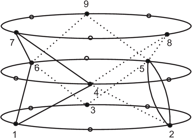
For example, consider the determinant of the Laplacian matrix of a cylinder of height 3 and perimeter 6 shown in Fig. 11. The set of vertices consists of filled circles marked by . The set of oriented edges is a collection of 24 inclined vectors of type . The corresponding Leibnitz expansion contains the term
| (52) |
which represents spanning digraphs on with 2 specified cycles and all possible oriented bonds outgoing from the vertices 3,8 and 9.
As noticed first in Ref. [19], the expansion (51) parallels in form the inclusion-exclusion principle in combinatorial mathematics. Indeed, let be the list of all possible proper cycles on , labeled in an arbitrary order. Define , as the set of all spanning digraphs on containing the particular cycle . Then, expansion (51) can be written in the form of the inclusion-exclusion principle:
| (53) |
which holds for any finite sets , where is the cardinality of the set . This sum equals zero, because all spanning digraphs on have at least one proper cycle , . The first term of the expansion originates from the term in Eq. (51) and represents the set of all possible cycles formed by oriented edges incident to every vertex of . To obtain the number of spanning webs, one has to subtract all the digraphs having contractible cycles and leave all those with noncontractible cycles wrapping the cylinder. To keep the number of noncontractible cycles, we have to change the weights of the nondiagonal terms in such a way that every cycle containing difference between the numbers of positive and negative steps equal to or , depending on the orientation, enters the determinant expansion with the opposite sign and sums up with the corresponding non-contractible cycle, generated by the arrows representing the diagonal term . At that, all the proper contractible cycles keep their sign in the expansion (51) in order to cancel out. This readily follows from the fact that every contractible cycle contains equal numbers of positive and negative steps. Thus, the matrix with elements given by (refelementsD) has all the necessary properties for the relationship (19) to define the proper generating function.
References
- [1] H.W.J. Blöte and B. Nienhuis, J. Phys. A 22, no. 9, 1415 (1989).
- [2] M.T. Batchelor, J. de Gier and B. Nienhuis, J. Phys. A 34, no.19, L265 (2001).
- [3] S. Mitra, B. Nienhuis, J. de Gier and M.T. Batchelor, J. Stat. Mech., P09010 (2004).
- [4] P.A. Pearce and J. Rasmussen, J. Stat. Mech., P02015 (2007).
- [5] H. Saleur, J. Phys. A 20, 455 (1987).
- [6] B. Duplantier, J. Phys. A 19, L1009 (1986).
- [7] H. Saleur, Nucl. Phys. B 382, 486 (1992).
- [8] P. A. Pearce, J. Rasmussen and S. Villani, J. Stat. Mech., P02010 (2010).
- [9] N. Sh. Izmailian, V. B. Priezzhev, Ph. Ruelle, and C.-K. Hu, Phys. Rev. Lett. 95, 260602 (2005).
- [10] D. Levy, Phys. Rev. Lett. 67, 1971 (1991); Int. J. Mod. Phys. A 6, 5127 (1991).
- [11] A. M. Gainutdinov, J. L. Jacobsen, N. Read, H. Saleur and R. Vasseur, J. Phys. A 46, 494012 (2013) and references therein; F. C. Alcaraz and V. Rittenberg, J. Stat. Mech., P09010 (2013); F. C. Alcaraz, P. Pyatov and V. Rittenberg, J. Phys. A 47, 462001 (2014).
- [12] P. Martin, Potts models and related problems in statistical mechanics, World Scientific (1990)
- [13] F. C. Alcaraz, M. N. Barber, and M. T. Batchelor, Ann. Phys. (NY) 182, 280 (1988).
- [14] C. Kirchhoff, Ann. Phys. Chem. 148, 497 (1847).
- [15] H. N. V. Temperley, in: London Math. Soc. Lecture Note Series, vol 13, Cambridge University Press, Cambridge, 1974, p.202.
- [16] P. W. Kasteleyn, Physica 27, 1209 (1961).
- [17] H. N. V. Temperley and M. E. Fisher, Philos. Mag. 6, 1061 (1961).
- [18] J. G. Brankov, S. Yu. Grigorev, V. B. Priezzhev, I. Y. Tipunin, J. Stat. Mech., P11017 (2008).
- [19] V. B. Priezzhev, Sov. Phys. Usp. 28, 1125 (1985).
- [20] A. Morin-Duchesne, P. A. Pearce, and J. Rasmussen, Nucl. Phys. B 874, 312 (2013).