Ensemble velocity of non-processive molecular motors with multiple chemical states

Andrej Vilfan Email: andrej.vilfan@ijs.si Affiliation: J. Stefan Institute, Jamova 39, 1000 Ljubljana, Slovenia Affiliation: Faculty of Mathematics and Physics, University of Ljubljana, Jadranska 19, 1000 Ljubljana, Slovenia

Abstract

We study the ensemble velocity of non-processive motor proteins, described with multiple chemical states. In particular, we discuss the velocity as a function of ATP concentration. Even a simple model which neglects the strain-dependence of transition rates, reverse transition rates and nonlinearities in the elasticity can show interesting functional dependencies, which deviate significantly from the frequently assumed Michaelis-Menten form. We discuss how the oder of events in the duty cycle can be inferred from the measured dependence. The model also predicts the possibility of velocity reversal at a certain ATP concentration if the duty cycle contains several conformational changes of opposite directionalities.

I Introduction

Motor proteins are molecular machines that convert chemical energy, usually obtained from the hydrolysis of ATP, to mechanical work by walking along their tracks [1, 2]. They can be classified as processive and non-processive [3]. Processive motors have the ability to make many steps before detaching from the track and a single motor molecule is sufficient to transport a cargo over a significant distance. In most cases processive motors are dimeric and alternately move their heads in a hand-over-hand fashion. Notable examples include most kinesins, myosin V, myosin VI and cytoplasmic dyneins. Non-processive motors dissociate from the track after each step, but can still move loads over long distances when cooperating in large numbers. Non-processivity is usually connected with a low duty ratio - the motor spends a large fraction of the cycle detached from the track. Best known non-processive motors are muscle myosins and axonemal dyneins. Many processive motors become non-processive in the monomeric form [4].

A number of studies has been devoted to the velocity of processive motors as a function of load and ATP concentration. For a processive motor one expects and finds that both the ATP hydrolysis rate and the velocity of the motor follow the Michaelis-Menten dependence on the ATP concentration [5, 6, 7, 8]

v=\frac{v_{\rm max}\rm[ATP]}{K_{m}+\rm[ATP]}\;.

(1)

The load dependence is more complex. Duke and Leibler proposed that some properties of kinesin’s force velocity relation could be explained even without any coordination of the two chemical cycles [9]. Alternatively, some models assume tight coordination and use the load dependence to construct diagrams with several states and mechanical substeps [10, 11].

In non-processive motors the situation is fundamentally different. Because each motor spends a significant part of its cycle in the detached state, the distance travelled per ATP hydrolyzed is not simply related to the step size. In fact, different estimates [12, 13, 14] of the distance per step led to a long lasting controversy about the myosin mechanism. Nevertheless, many models for muscle myosin were developed, aimed at relating the velocity or transient response of muscle sarcomeres to the properties of a single myosin molecule [15, 16, 17]. They were able to predict the principal features of the myosin cycle long before any structural evidence was available. The aforementioned models studied the limit of a large number of motors and assumed that the filaments are sliding at a constant velocity. In other words, they excluded the possibility that the cycles of motors become correlated and produce non-uniform motion. This possibility was explored by Duke [18, 19] who showed that a filament under high load can indeed show a synchronization of chemical cycles between myosin heads and step-wise motion. A further complication arises from the structure of a muscle fibril with many sarcomeres in series. This can cause spontaneous symmetry breaking and individual motors can be subject to a different stretch than the macroscopic sarcomere [20]. The application of an abrupt force step can transiently synchronize the motors and lead to observable oscillations [21], as predicted by Duke’s model.

Refer to caption — Figure 1: Duty cycle of a motor, consisting of $N$ bound states with distinct lever orientations and irreversible transitions between them. A detached motor (state D) binds to the track with rate $k_{\rm on}$ , which leads to state 1 and the elastic element is initially unstrained. The next transition ( $1\to 2$ ) takes place with the rate $k_{1}$ and includes a lever arm movement of distance $d_{1}$ . Eventually, the motor detaches from state $N$ with the rate $k_{\rm off}$ .

Less attention has been paid to the velocity of non-processive motors as a function of the ATP concentration. It is frequently assumed to follow a Michaelis-Menten like dependence, as would be the case with processive motors, even though there is no reason why it should have that form. Some experimental studies on myosins either show no deviation from the Michaelis-Menten shape [22, 23, 24, 25, 26, 27], whereas others show minor, but significant deviation [28]. Axonemal dyneins also largely follow the Michaelis-Menten dependence [29, 30]. An expression for a specific model has been discussed in the seminal paper by Leibler and Huse [31]. They show that the dependence is described by a more complex function, which they call generalized Michaelis-like law. However, the dependence still has a similar functional form – as we will see this is related to the assumption that the power stroke takes place as the next step after binding.

The aim of this paper is to discuss the dependence $v(\rm[ATP])$ in a more general context. The study is motivated by other non-processive motors that do not necessarily have a power-stroke right after binding. We can mention non-processive kinesins [32] (e.g., kinesin-14 or ncd [33]) as examples of such motors. Because the ATP dependence of the velocity can be measured in a relatively simple motility assay [34], our model should provide a way to extract some properties of the duty cycle that are difficult to measure in a single-molecule experiment.

II Model

In the following we will discuss a generalization of the “rower” model [31] by introducing several substeps. On the other hand, we still make a number of simplifying assumptions, notably that all elastic elements are linear, that the chemical transitions are irreversible and their rates independent of strain. We further assume that the motors always run through the same cycle, which involves hydrolysis of 1 ATP molecule. All these simplifications are limited in their validity, but should work well in a motility assay where forces are relatively small. As a rule of thumb, the strain dependence of transition rates can be neglected if the elastic energy change during a step is smaller than the thermal energy. This will be the case if the motors are attached with their flexible tails to the glass surface. For example, different single-molecule studies report myosin’s elastic constant as $0.7\,\rm pN/nm$ for full length HMM [35], but $1.8\,\rm pN/nm$ for the S1 fragment lacking the tail [36]. In a muscle sarcomere the tails are tightly packed into thick filaments, which also increases their effective stiffness [37]. The assumption of linear elastic elements will also hold for relatively small forces that are exerted by motors in a motility assay. Finally, neglecting reverse transitions in the cycle is valid if there is no ADP and phosphate in solution (which would lead to reversal of product release steps) and, again, if the forces are too low for significant mechanically induced reverse transitions. In a recent paper Persson et al. [27] discuss the role of the aforementioned effects in a motility assay for rather stiffly anchored heads ( $2.8\,\rm pN/nm$ ) and show that off-path transitions and nonlinear elasticity can be important, although the resulting dependence is close to the Michaelis-Menten form. We further assume that the filaments (or tracks) are straight and stiff, and that all motors interacting with them all act in the same way and move the filament along its axis.

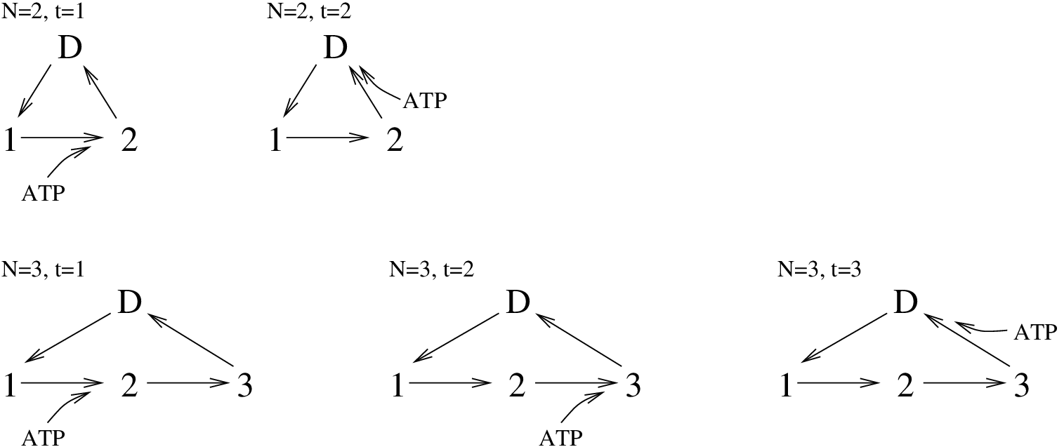
The motors are modelled as shown in Fig. 1. We assume that each motor is connected through an elastic element (spring constant $K$ ) to the backbone (or surface in a motility assay). The motor is initially in the dissociated state (state D). It binds to the track with the rate $k_{\rm on}$ . After that it undergoes its first conformational change with a rate $k_{1}$ , which moves the lever by a distance $d_{1}$ . The next step, taking place with a rate $k_{2}$ moves it by $d_{2}$ , … until it reaches the last bound state $N$ from where it detaches with a rate $k_{\rm off}$ . We denote the average dwell times in those states with $\tau_{1}=1/k_{1}$ , …, $\tau_{N}=1/k_{\rm off}$ and $\tau_{\rm det}=1/k_{\rm on}$ . One of the steps requires binding of ATP and is therefore a second-order transition. If this is the constant $k_{t}$ , the corresponding dwell time is $\tau_{t}=1/(k_{t}\rm[ATP])$ .

In the above scheme 1 ATP molecule is always hydrolyzed per cycle and the ATPase rate per motor can be expressed as

v_{\rm ATPase}=\frac{1}{\tau_{\rm det}+\sum_{i=1}^{N}\tau_{i}}=\frac{1}{\tau_{\rm det}+\sum_{i\neq t}\tau_{i}+1/(k_{t}{\rm[ATP]})}\;,

(2)

which always follows the Michaelis-Menten dependence.

In the following we will derive the velocity of a large ensemble of motors acting between the same backbone and track. In the limit of a large motor number, $n\to\infty$ , the motion becomes uniform and the velocity fluctuations due to random transitions in individual motors negligible (simulation results for finite sized systems are shown in Appendix A). We can examine the steady state of the system by assuming a constant velocity $v$ , then calculating the average force produced by each motor and finally determining $v$ from force equilibrium.

With $\xi$ we denote the position of the lever arm relative to state 1, i.e., it has the values $\xi=0$ in state 1, $\xi=d_{1}$ in state 2, $\xi=d_{1}+d_{2}$ in state 3, and so on. The ensemble average of $\xi$ among all bound motors is then

\langle\xi\rangle=\frac{\sum_{i=2}^{N}\sum_{j=1}^{i-1}d_{j}\tau_{i}}{\sum_{i=1}^{N}\tau_{i}}\;.

(3)

As the track is moving with velocity $v$ , the average strain on a spring is reduced by the expectation value of $\langle vt\rangle$ among bound motors, where $t$ is the time passed since initial binding. It can be calculated using

\langle t\rangle=\frac{\int_{0}^{\infty}P(t)t\,dt}{\int_{0}^{\infty}P(t)dt}=\frac{\sum_{i=1}^{N}\int_{0}^{\infty}P_{i}(t)t\,dt}{\sum_{i=1}^{N}\int_{0}^{\infty}P_{i}(t)dt}

(4)

where $P(t)$ is the probability that the motor is still attached at time $t$ after its initial attachment and $P_{i}(t)$ is the probability that it is in $i$ -th bound state. The integrals are $\int_{0}^{\infty}P_{i}(t)dt=\tau_{i}$ and $\int_{0}^{\infty}P_{i}(t)t\,dt=(\tau_{1}+\tau_{2}+\ldots+\tau_{i})\tau_{i}$ . Together, these expressions give us the value

\langle x\rangle=\langle vt\rangle=v\frac{\sum_{i=1}^{N}\sum_{j=1}^{i}\tau_{i}\tau_{j}}{\sum_{i=1}^{N}\tau_{i}}\;.

(5)

The total force produced by all motors can be expressed as

F=\langle n\rangle K(\langle\xi\rangle-\langle x\rangle)

(6)

with $n$ denoting the number of attached motors,

n=n_{\rm tot}\left(1-\frac{\tau_{\rm det}}{\sum_{i=1}^{N}\tau_{i}+\tau_{\rm det}}\right)\;.

(7)

In a gliding assay the friction is generally negligible and the force equilibrium states $F=0$ . From Eq. (6) it follows that $\langle\xi\rangle=\langle x\rangle$ and we obtain an expression for the velocity

v=\frac{\sum_{i=2}^{N}\sum_{j=1}^{i-1}d_{j}\tau_{i}}{\sum_{i=1}^{N}\sum_{j=1}^{i}\tau_{i}\tau_{j}}\;.

(8)

In the following we will discuss the properties of this equation.

II.1 Model with two bound states

The simplest non-trivial case involves $N=2$ bound states (Fig. 2, upper row): the first directly after binding and the second after a power stroke of distance $d_{1}$ . The expression for velocity simplifies to

v=\frac{d_{1}\tau_{2}}{\tau_{1}^{2}+\tau_{1}\tau_{2}+\tau_{2}^{2}}

(9)

If ATP binds on the second transition ( $t=2$ ) we get the following concentration dependence (Fig. 3a):

v=\frac{d_{1}k_{t}\rm[ATP]}{1+(k_{t}/k_{1}){\rm[ATP]}+((k_{t}/k_{1}){\rm[ATP]})^{2}}

(10)

As expected, this dependence is linear at low ATP concentrations, but the velocity somewhat surprisingly drops at high ATP concentrations, too. The reason is that the post-powerstroke state becomes short lived and motors produce forward force only for a small fraction of time. The maximum velocity $v_{\rm max}=d_{1}k_{1}/3$ is achieved at ${\rm[ATP]}=k_{1}/k_{t}$ . The non-monotonic dependence shows that the model is not adequate to describe the properties of muscle myosin, which needs at least two post-powerstroke states (ADP and rigor).

The second possibility is that ATP binding is the first step ( $t=1$ ). Then the expression for velocity is (Fig. 3b):

v=\frac{d_{1}k_{\rm off}((k_{t}/k_{\rm off})\rm[ATP])^{2}}{1+(k_{t}/k_{\rm off}){\rm[ATP]}+((k_{t}/k_{\rm off}){\rm[ATP]})^{2}}

(11)

The dependence is quadratic at low ATP concentrations. In this regime the ensemble of bound motors is dominated by motors in the pre-powerstroke state waiting for ATP binding. An increasing ATP concentration not only accelerates the cycling rate, but also increases the fraction of post-powerstroke motors in the ensemble, hence quadratic dependence. The maximum velocity at saturating [ATP] is $v_{\rm max}=d_{1}k_{\rm off}$ and half the maximum is reached at ${\rm[ATP]}=\varphi\frac{k_{\rm off}}{k_{t}}$ , where $\varphi=(1+\sqrt{5})/2$ represents the golden ratio.

This simple model with 2 bound states demonstrates that the velocity shows a dependence that is profoundly different from the frequently used Michaelis-Menten like dependence. It also allows us to determine whether the power stroke takes place before or after ATP binding.

II.2 Model with three bound states

In the following, we allow $N=3$ consecutive bound states (Fig. 2, lower row). The lever movements are $d_{1}$ (between 1 and 2) and $d_{2}$ (between 2 and 3). Again, we have to distinguish between schemes where ATP binds to the first, second or third state.

If ATP binding is the first transition ( $t=1$ ), the expression for the velocity reads

v=\frac{d_{1}/k_{2}+(d_{1}+d_{2})/k_{\rm off}}{1/(k_{t}{\rm[ATP]})^{2}+(1/k_{2}+1/k_{\rm off})/(k_{t}{\rm[ATP]})+1/k_{2}^{2}+1/k_{\rm off}^{2}+1/(k_{2}k_{\rm off})}\;.

(12)

The functional dependence of this equation is similar to Eq. (11). The deviation is maximal when $k_{2}=k_{\rm off}$ , but even in this case the difference never exceeds $0.008\,v_{\rm max}$ . (Fig. 4a).

The situation becomes different if ATP binding is the second step, $t=2$ . Then we get

v=\frac{d_{1}/(k_{t}{\rm[ATP]})+(d_{1}+d_{2})/k_{\rm off}}{1/(k_{t}{\rm[ATP]})^{2}+(1/k_{1}+1/k_{\rm off})/(k_{t}{\rm[ATP]})+1/k_{1}^{2}+1/k_{\rm off}^{2}+1/(k_{1}\ k_{\rm off})}

(13)

In the special case $d_{1}=0$ the ATP waiting state becomes pre-powerstroke and the functional form is the same as (12). We expect that this scenario describes the cycle of single-headed kinesin, which binds to the microtubule in ADP state, releases ADP, binds ATP and docks the neck linker (which effectively represents a power stroke of distance $d_{2}$ ), hydrolyzes ATP and detaches [38, 39].

Alternatively, for $d_{2}=0$ Eq. (13) represents the “Michaelis-like law”, as identified by Leibler and Huse [31] (Fig. 4b). At high ATP concentrations the velocity approaches the saturation value faster and, depending on parameter values, may also overshoot for the same reason as the two-state model (Eq. 11).

Equation (13) becomes particularly interesting if $d_{1}$ and $d_{1}+d_{2}$ have opposite signs (we assign $d_{1}<0$ ). This means that the motor first binds, makes a conformational change in negative direction, waits for ATP to bind and then commits the actual power stroke in the positive direction. The velocity then changes direction at a certain ATP concentration. At low concentrations, the motors move in the direction of $d_{1}$ and at high concentrations in the direction of $d_{1}+d_{2}$ . Examples of such curves are shown in Fig. 5.

Finally, if ATP binding is the third step and triggers detachment ( $t=3$ ), the velocity is given by

v=\frac{d_{1}/k_{2}+(d_{1}+d_{2})/(k_{t}{\rm[ATP]})}{1/(k_{t}{\rm[ATP]})^{2}+(1/k_{1}+1/k_{2})/(k_{t}{\rm[ATP]})+1/k_{1}^{2}+1/k_{2}^{2}+1/(k_{1}\ k_{2})}\;.

(14)

The properties of this expression are similar to the case when ATP binding is the second step. We expect that this expression should describe the dependence for muscle myosin (myosin II), whose main bound states are A.M.ADP.Pi, A.M.ADP and A.M [40, 41]. The main power stroke ( $d_{1}$ ) takes place along with phosphate release, but there is a second, smaller conformational change upon ADP release ( $d_{2}$ ). Single molecule experiments give values of $d_{1}\approx 5\,\rm nm$ (which is possibly an underestimate [42]) and $d_{2}\approx 1-2\,\rm nm$ [43, 44].

III Conclusions

With this simple model we could show that the collective motor velocity, for example measured in a gliding assay, can show non-trivial dependence on the ATP concentration. A careful examination of its limiting cases (low and high [ATP]) can reveal details about the duty cycle that would otherwise require single molecule measurements which are not only more demanding, but also more affected by thermal noise. In particular, we show that a force-velocity relationship that resembles the Michaelis-Menten shape (1) indicates that the motor has at least 3 bound states and that ATP binding occurs after the power stroke. We would expect this and largely find it for muscle myosin [22, 23, 24, 25, 26, 27] and various dyneins [29, 30]. A quadratic dependence, on the other hand, is the signature of ATP binding before the power stroke. This could apply to non-processive kinesin family motors, even though some available diagrams [45] do not yet show a visible difference.

A particularly interesting aspect of the model is the theoretical possibility that a motor could reverse its direction depending on the ATP concentration. To our knowledge, no such behaviour has been reported in natural motor proteins so far. There are, however, kinesin-5 Cin8 that switches direction depending on the ionic strength [46, 47] and dynein that reverses upon addition of phosphate [48]. Notable achievements involving artificial inversion and/or direction switching include an insertion in the myosin lever arm that reversed its direction [49] and a myosin construct that can switch direction depending on the calcium concentration [50]. The possibilities to engineer motor molecules should eventually allow an adjustment of lever displacements in individual states and creation of a motor whose direction of motion would depend on the ATP concentration.

Finally, the same approach that we used here to describe the longitudinal motion could also be used for rotational motion of filaments, driven by lateral power-strokes in motor proteins. Filament rotation by non-processive myosins can be caused by the fact that for steric reasons a myosin head can only bind to certain “target zones” on an actin filament [51], but in addition myosin can have an off-axis component of the power stroke. The interplay between the two-contributions could lead to a cross-over from left- to right handed rotation depending on the ATP concentration. In addition, if a motor has several lateral power strokes, this alone could already lead to complex dependencies of the helical pitch on the ATP concentration.

Acknowledgements.

This work was supported by Slovenian Research Agency (Grant P1-0099 and J1-5437).

Appendix A Simulation of finite ensembles

In order to validate the steady state assumption on which the theory in this paper is based, we show some simulation results on a finite ensemble of motors in this Appendix. All results were obtained with a kinetic Monte Carlo simulation (Gillespie algorithm) on a system of $n$ rigidly coupled motors with the same properties as described in the main text. For the sake of simplicity, all simulations were carried out with $\tau_{\rm det}=0$ (corresponding to $k_{\rm on}\to\infty$ ), which means that a group of $n=2$ motors is already processive (i.e., the two motors will not detach from the track simultaneously). Figure 6 shows the velocities for the same parameters as in Figs. 4 and 5, but with finite numbers ( $n=2,5,10,20$ ) of motors. Although very small groups ( $n=2$ ) show some significant deviation, the analytical result becomes almost exact for $n\gtrsim 10$ motors.

References

[1] J. Howard, Mechanics of Motor Proteins and the Cytoskeleton (Sinauer, Sunderland, MA, 2001).
[2] A. B. Kolomeisky and M. E. Fisher, Annu. Rev. Phys. Chem. 58, 675 (2007).
[3] J. Howard, Nature 389, 561 (1997).
[4] W. O. Hancock and J. Howard, J. Cell. Biol. 140, 1395 (1998).
[5] J. Howard, A. J. Hudsepth, and R. D. Vale, Nature 342, 154 (1989).
[6] G. Steinberg and M. Schliwa, J. Biol. Chem. 271, 7516 (1996).
[7] M. J. Schnitzer and S. M. Block, Nature 388, 386 (1997).
[8] K. Visscher, M. J. Schnitzer, and S. M. Block, Nature 400, 184 (1999).
[9] T. Duke and S. Leibler, Biophys. J. 71, 1235 (1996).
[10] M. E. Fisher and A. B. Kolomeisky, Proc. Natl. Acad. Sci. USA 98, 7748 (2001).
[11] D. Tsygankov and M. E. Fisher, Proc. Natl. Acad. Sci. USA 104, 19321 (2007).
[12] Y. Y. Toyoshima, S. J. Kron, and J. A. Spudich, Proc. Natl. Acad. Sci. USA 87, 7130 (1990).
[13] T. Q. Uyeda, S. J. Kron, and J. A. Spudich, J. Mol. Biol. 214, 699 (1990).
[14] Y. Harada and T. Yanagida, Cell Motil. Cytoskeleton 10, 71 (1988).
[15] A. F. Huxley, Prog. Biophys. Biophys. Chem. 7, 255 (1957).
[16] T. L. Hill, Prog. Biophys. Mol. Biol. 28, 267 (1974).
[17] E. Eisenberg, T. L. Hill, and Y. Chen, Biophys. J. 29, 195 (1980).
[18] T. A. J. Duke, Proc. Natl. Acad. Sci. USA 96, 2770 (1999).
[19] T. Duke, Philos. Trans. R. Soc. Lond. B Biol. Sci. 355, 529 (2000).
[20] A. Vilfan and T. Duke, Biophys. J. 85, 818 (2003).
[21] K. A. P. Edman and N. A. Curtin, J. Physiol. 534, 553 (2001).
[22] S. J. Kron and J. A. Spudich, Proc. Natl. Acad. Sci. USA 83, 6272 (1986).
[23] D. M. Warshaw, J. M. Desrosiers, S. S. Work, and K. M. Trybus, J. Biol. Chem. 266, 24339 (1991).
[24] E. P. Debold, S. E. Beck, and D. M. Warshaw, Am. J. Physiol. Cell Physiol. 295, C173 (2008).
[25] E. P. Debold, M. A. Turner, J. C. Stout, and S. Walcott, Am. J. Physiol. Regul. Integr. Comp. Physiol. 300, R1401 (2011).
[26] M. Canepari, M. Maffei, E. Longa, M. Geeves, and R. Bottinelli, Exp. Physiol. 97, 873 (2012).
[27] M. Persson, E. Bengtsson, L. ten Siethoff, and A. Mansson, Biophys. J. 105, 1871 (2013).
[28] J. E. Baker, C. Brosseau, P. B. Joel, and D. M. Warshaw, Biophys. J. 82, 2134 (2002).
[29] O. Kagami and R. Kamiya, J. Cell Sci. 103, 653 (1992).
[30] D. P. Lorch, C. B. Lindemann, and A. J. Hunt, Cell Motil. Cytoskeleton 65, 487 (2008).
[31] S. Leibler and D. Huse, J. Cell. Biol. 121, 1357 (1993).
[32] R. A. Cross and A. McAinsh, Nat. Rev. Mol. Cell. Biol. 15, 257 (2014).
[33] R. A. Cross, BMC Biol. 8, 107 (2010).
[34] T. Duke, E. Holy, and S. Leibler, Phys. Rev. Lett. 74, 330 (1995).
[35] C. Veigel, M. L. Bartoo, C. S. White, J. S. Sparrow, and J. E. Molloy, Biophys. J. 75, 1424 (1998).
[36] A. Lewalle, W. Steffen, O. Stevenson, Z. Ouyang, and J. Sleep, Biophys. J. 94, 2160 (2008).
[37] M. Kaya and H. Higuchi, Cell. Mol. Life Sci. 70, 4275 (2013).
[38] A. Hoenger, M. Thormählen, R. Diaz-Avalos, M. Doerhoefer, K. Goldie, J. Müller, and E. Mandelkow, J. Mol. Biol. 297, 1087 (2000).
[39] N. R. Guydosh and S. M. Block, Nature 461, 125 (2009).
[40] R. W. Lymn and E. W. Taylor, Biochemistry 10, 4617 (1971).
[41] E. Pate and R. Cooke, J. Muscle Res. Cell Motil. 10, 181 (1989).
[42] J. Sleep, A. Lewalle, and D. Smith, Proc. Natl. Acad. Sci. USA 103, 1278 (2006).
[43] C. Veigel, J. E. Molloy, S. Schmitz, and J. Kendrick-Jones, Nat. Cell Biol. 5, 980 (2003).
[44] M. Capitanio, M. Canepari, P. Cacciafesta, V. Lombardi, R. Cicchi, M. Maffei, F. S. Pavone, and R. Bottinelli, Proc. Natl. Acad. Sci. USA 103, 87 (2006).
[45] M. J. deCastro, C. H. Ho, and R. J. Stewart, Biochemistry 38, 5076 (1999).
[46] J. Roostalu, C. Hentrich, P. Bieling, I. A. Telley, E. Schiebel, and T. Surrey, Science 332, 94 (2011).
[47] A. Gerson-Gurwitz, C. Thiede, N. Movshovich, V. Fridman, M. Podolskaya, T. Danieli, S. Lakamper, D. R. Klopfenstein, C. F. Schmidt, and L. Gheber, EMBO J. 30, 4942 (2011).
[48] W. J. Walter, M. P. Koonce, B. Brenner, and W. Steffen, Proc. Natl. Acad. Sci. USA 109, 5289 (2012).
[49] G. Tsiavaliaris, S. Fujita-Becker, and D. J. Manstein, Nature 427, 558 (2004).
[50] L. Chen, M. Nakamura, T. D. Schindler, D. Parker, and Z. Bryant, Nat. Nanotechnol. 7, 252 (2012).
[51] A. Vilfan, Biophys. J. 97, 1130 (2009).