On a Class of Nonlocal Wave Equations
from Applications

Horst Reinhard Beyer¹¹ 1 Department of Mathematics, TOBB University of Economics and Technology, Ankara, 06560, Turkey & Instituto Tecnológico Superior de Uruapan, Carr. Uruapan-Carapan No. 5555, Col. La Basilia, Uruapan, Michoacán. México & Theoretical Astrophysics, IAAT, Eberhard Karls University of Tübingen, Tübingen 72076, Germany, hbeyer@etu.edu.tr. Burak Aksoylu²² 2 Department of Mathematics, TOBB University of Economics and Technology, Ankara, 06560, Turkey & Department of Mathematics and Statistics, University of New Mexico, Albuquerque, NM 87131, USA, baksoylu@etu.edu.tr. This work was supported in part by National Science Foundation DMS 1016190 grant, European Commission Marie Curie Career Integration Grant 293978, and Scientific and Technological Research Council of Turkey (TÜBİTAK) TBAG 112T240 and MAG 112M891 grants. Research visit of Horst R. Beyer was supported in part by TÜBİTAK 2221 Fellowship for Visiting Scientist Program. Sabbatical visit of Fatih Celiker was supported in part by TÜBİTAK 2221 Fellowship for Scientist on Sabbatical Leave Program. and Fatih Celiker³³ 3 Department of Mathematics, Wayne State University, 656 W. Kirby, Detroit, MI 48202, USA, celiker@math.wayne.edu. This work was supported in part by National Science Foundation DMS 1115280 grant.
August 24, 2026

Abstract

We study equations from the area of peridynamics, which is an extension of elasticity. The governing equations form a system of nonlocal wave equations. Its governing operator is found to be a bounded, linear and self-adjoint operator on a Hilbert space. We study the well-posedness and stability of the associated initial value problem. We solve the initial value problem by applying the functional calculus of the governing operator. In addition, we give a series representation of the solution in terms of spherical Bessel functions. For the case of scalar valued functions, the governing operator turns out as functions of the Laplace operator. This result enables the comparison of peridynamic solutions to those of classical elasticity as well as the introduction of local boundary conditions into the nonlocal theory. The latter is studied in a companion paper.

keywords

Nonlocal wave equation, nonlocal operators, peridynamics, elasticity, operator theory.

AMS

47G10, 35L05, 74B99

August 24, 2026

1 Motivation

Classical elasticity has been successful in characterizing and measuring the resistance of materials to crack growth. On the other hand, peridynamics (PD), a nonlocal extension of continuum mechanics developed by Silling [63], is capable of quantitatively predicting the dynamics of propagating cracks, including bifurcation. Its effectiveness has been established in sophisticated applications such as Kalthoff-Winkler experiments of the fracture of a steel plate with notches [36, 64], fracture and failure of composites, nanofiber networks, and polycrystal fracture [38, 52, 66, 65]. Further applications are in the context of multiscale modeling, where PD has been shown to be an upscaling of molecular dynamics [60, 62] and has been demonstrated as a viable multiscale material model for length scales ranging from molecular dynamics to classical elasticity [10]. Also see other related engineering applications [14, 37, 39, 54, 53], the review and news articles [16, 21, 43] for a comprehensive discussion, and the recent book [45].

We study a class of nonlocal wave equations. The driving application is PD. The same operator is also employed in nonlocal diffusion [9, 16, 59]. Similar classes of operators are used in numerous applications such as population models [13, 50], image processing [31, 40], particle systems [12], phase transition [8, 7], and coagulation [30]. In addition, we witness a major effort to meet the need for mathematical theory for PD applications and related nonlocal problems addressing, for instance, conditioning analysis, domain decomposition and variational theory [3, 4, 5], volume constraints [16, 18, 17], nonlinearity [24, 25, 26, 44], discretization [1, 5, 29, 68], numerical methods [15, 19, 22, 58], and various other aspects [6, 20, 23, 27, 28, 32, 33, 41, 42, 46, 47, 48, 60, 61, 72].

It is part of the folklore in physics that the point particle model, which is the root for locality in physics, is the cause of unphysical singular behavior in the description of the underlying phenomena. This fact is a strong indication that, in the long run, the development of nonlocal theories is necessary for description of natural phenomena. Operator theory does not discern the locality or nonlocality of the governing operator. This is the strength of this approach. This article adds valuable tools to the arsenal of methods to analyze nonlocal problems, thereby, increasing structural understanding in the field.

The rest of the article is structured as follows. We start with a mathematical introduction in Section 1.1. In Section 2, we set the operator theory framework to treat the nonlocal wave equation. We prove basic properties of the solutions such as well-posedness of the initial value problem and provide a representation of the solutions in terms of bounded functions of the governing operator. We study the stability of solutions and give conservation laws. In Section 3, in the vector-valued case, we note that the governing operator becomes an operator matrix. The generality of operator theory allows a simple extension of the results established for the scalar-valued functions to the vector-valued ones. We prove the boundedness of the entries of the governing operator matrix. The proof is natural due to operator theory again, because it relies on a well-known criterion for integral operators. We present a “diagonalization” of the matrix entries. This is accomplished by employing the unitary Fourier transform and connecting the entries to maximal multiplication operators. We study the spectral properties of the entries. Then, we reach to a notable result. Namely, we prove that the governing operator is a bounded function of the classical local operator. This has far reaching consequences. It enables the incorporation of local boundary conditions into nonlocal theories, which is the subject of our companion paper [2]. We introduce notion of strong resolvent convergence. This allows us to prove the convergence of solutions of the governing equation to that of the classical solution. We give examples of sequences of micromoduli that are instance of this result. In Section 4, we consider the calculation of the solution of the wave equation. Since the governing operator is bounded, holomorphic functions of that operator can be represented in form of power series in the operator. Then, we give a representation of holomorphic functions, present in the solution of the initial value problem, utilizing the fact that the governing operator is a sum of two commuting operators. We discover that the corresponding power series can be given in terms of a series of Bessel functions. In Section 5, we apply the representation in terms of Bessel functions to special Gaussian micromoduli and Gaussian data. We depict the resulting solutions of peridynamic wave equation and compare to the classical solutions. We conclude in Section 6.

1.1 Mathematical Introduction

The formal system of linear peridynamic wave equations in $n$ -space dimensions [63, Eqn. 54] $n\in{\mathbb{N}}^{*}$ , is given by

\rho\,\frac{\partial^{2}u}{\partial t^{2}}(x,t)=\int_{{\mathbb{R}}^{n}}C(x^{\prime}-x)\cdot\left(u(x^{\prime},t)-u(x,t)\right)dx^{\prime}+b(x,t)\,\,,

(1.1)

where “ $\cdot$ ” indicates matrix multiplication, or equivalently by the system

\rho\,\frac{\partial^{2}u_{j}}{\partial t^{2}}(x,t)=\sum_{k=1}^{n}\int_{{\mathbb{R}}^{n}}C_{jk}(x^{\prime}-x)\cdot\left(u_{k}(x^{\prime},t)-u_{k}(x,t)\right)dx^{\prime}+b_{j}(x,t)\,\,,

(1.2)

where $x\in{\mathbb{R}}^{n}$ , $t\in{\mathbb{R}}$ , $C:{\mathbb{R}}^{n}\rightarrow M(n\times n,{\mathbb{R}})$ is the micromodulus tensor, assumed to be even and assuming values inside the subspace of symmetric matrices, $\rho>0$ is the mass density, $b:{\mathbb{R}}^{n}\times{\mathbb{R}}\rightarrow{\mathbb{R}}^{n}$ is the prescribed body force density, and $u:{\mathbb{R}}^{n}\times{\mathbb{R}}\rightarrow{\mathbb{R}}^{n}$ is the displacement field.

For comparison, e.g., the corresponding wave equation in classical elasticity in $1$ -space dimension is given by

\rho\,\frac{\partial^{2}u}{\partial t^{2}}=E\,\frac{\partial^{2}u}{\partial x^{2}}+b\,\,,

(1.3)

where $E>0$ is the so called “Young’s modulus,” and describing compression waves in a rod.

If $j,k\in\{1,\dots,n\}$ and $C_{jk}\in L^{1}({\mathbb{R}}^{n})$ , we can rewrite (1.2) as

\rho\,\frac{\partial^{2}u_{j}}{\partial t^{2}}(x,t)=-\sum_{k=1}^{n}\left\{\,\left[\int_{{\mathbb{R}}^{n}}C_{jk}(x^{\prime})dx^{\prime}\right]u_{k}(x,t)-(C_{jk}*u_{k}(\cdot,t))(x)\right\}+b_{j}(x,t)\,\,,

(1.4)

for all $x\in{\mathbb{R}}^{n}$ , $t\in{\mathbb{R}}$ and $j\in\{1,\dots,n\}$ where $*$ denotes the convolution product. The system (1.4) is the starting point for a functional analytic interpretation, which leads on a well-posed initial value problem. For this purpose, we use methods from operator theory; see, e.g., [11, 55].

2 Operator-Theoretic Treatment of Systems of Wave Equations

Analogous to the majority of evolution equations from classical and quantum physics, (1.4) can be treated with methods from operator theory, see, e.g., [11, 55] for substantiation of this claim and [34] for applications of operator theory in engineering. More specifically, this system falls into the class of abstract linear wave equations from Theorem 2.1. For the proof of this theorem see, e.g., [11, Thm. 2.2.1 and Cor. 2.2.2]. Special cases of this theorem are proved in [35, 49] and [56, Vol. II]. Statements and proofs make use of the spectral theorems of (densely-defined, linear and) self-adjoint operators in Hilbert spaces, including the concept of functions of such operators, see, e.g., [56, Vol. I], or standard books on Functional Analysis, such as [57, 71]. These methods are also used throughout the paper.

This section provides the basic properties of the solutions of abstract wave equations of the form (2.1). Some of the subsequent results are scattered in the literature. Therefore, wherever necessary, we provide proofs. In particular, Theorem 2.1 gives the well-posedness of the initial value problem for a class of abstract wave equations, conservation of energy and a representation of the solutions in terms of bounded functions of the governing operator. Corollary 2.2 and Theorem 2.3 are results on the stability of the solutions, i.e., their growth for large times. Theorem 2.4 provides conservation laws induced by symmetries of the governing operator. Theorem 2.5 provides special solutions of the associated class of inhomogeneous wave equations. Together with Theorem 2.1, these solutions provide the well-posedness of the initial value problem of the latter equations as well as a representation of the solutions in terms of bounded functions of the governing operator.

Theorem 2.1.

(Wave Equations) Let $\left(X,\braket{|}\right)$ be some non-trivial complex Hilbert space. Furthermore, let $A:D(A)\rightarrow X$ be some densely-defined, linear, semibounded self-adjoint operator in $X$ with spectrum $\sigma(A)$ . Finally, let $\xi,\eta\in D(A)$ .

(i)

Then there is a unique twice continuously differentiable map $u:{\mathbb{R}}\rightarrow X$ assuming values in $D(A)$ and satisfying

$u^{\,\prime\prime}(t)=-A\,u(t)$ (2.1)

for all $t\in{\mathbb{R}}$ as well as

$u(0)=\xi\,\,,\,\,u^{\,\prime}(0)=\eta\,\,.$
(ii)

For this $u$ , the corresponding energy function $E_{u}:\mathbb{R}\rightarrow{\mathbb{R}}$ , defined by

$E_{u}(t):=\frac{1}{2}\,\big(\,\braket{u^{\,\prime}(t)|u^{\,\prime}(t)}+\braket{u(t)|Au(t)}\,\big)$

for all $t\in{\mathbb{R}}$ , is constant.

(iii)

Moreover, this $u$ is given by

u(t)=\left[\overline{\cos\left(t\sqrt{\phantom{ij}}\right)}\,\bigg|_{\sigma(A)}\right]\!(A)\xi+\left[\,\overline{\frac{\sin\left(t\sqrt{\phantom{ij}}\right)}{\sqrt{\phantom{ij}}}}\,\bigg|_{\sigma(A)}\right]\!(A)\eta

(2.2)

for all $t\in{\mathbb{R}}$ , where

\overline{\cos(t\sqrt{\phantom{ij}}\,)}\,\,\,\,\textrm{and}\,\,\,\,\overline{\frac{\sin(t\sqrt{\phantom{ij}}\,)}{\sqrt{\phantom{ij}}}}

denote the unique extensions of $\cos(t\sqrt{\phantom{ij}}\,)\,\,\,\,\textrm{and}\,\,\,\,\sin(t\sqrt{\phantom{ij}})/\sqrt{\phantom{ij}},$ respectively, to entire holomorphic functions.

Moreover, if $A$ is positive, the solutions of (2.1) are stable, i.e., there are no solutions that are growing exponentially in the norm.

Corollary 2.2.

(Stability of Solutions) If $A$ is positive, then

\|u(t)\|\leqslant\|\xi\|+|t|\cdot\|\eta\|

for every $t\in{\mathbb{R}}$ .

Proof.

The statement follows from Theorem 2.1 (iii), since, from an application of the spectral theorem of densely-defined, linear and self-adjoint operators in Hilbert spaces, it follows that the operator norms of the operators in (2.2) satisfy

\bigg\|\left[\overline{\cos\left(t\sqrt{\phantom{ij}}\right)}\,\bigg|_{\sigma(A)}\right]\!(A)\bigg\|\leqslant 1\,\,,\,\,\bigg\|\left[\,\overline{\frac{\sin\left(t\sqrt{\phantom{ij}}\right)}{\sqrt{\phantom{ij}}}}\,\bigg|_{\sigma(A)}\right]\!(A)\bigg\|\leqslant t\,\,,

for every $t\in{\mathbb{R}}$ . ∎

On the other hand, if $A$ is strictly negative, there are solutions of (2.1) that are growing exponentially in the norm. The corresponding theorem is not readily found in the literature. For the convenience of the reader, we give a proof in the Appendix.

Theorem 2.3.

(Instability of Solutions) If $\left(X,\braket{|}\right)$ , $A:D(A)\rightarrow X$ , $\sigma(A)$ are as in Theorem 2.1 and, in addition, $A$ is such that

\sigma(A)\cap(-\infty,0)\neq\emptyset\,\,,

then there is a twice continuously differentiable map assuming values in $D(A)$ and satisfying

u^{\,\prime\prime}(t)=-A\,u(t)

for all $t\in{\mathbb{R}}$ with exponentially growing norm.

Proof.

See the Appendix. ∎

The following Theorem 2.4 can be considered a form of Noether’s Theorem for the solutions of (2.1). For the convenience of the reader, we provide a proof in the Appendix.

Theorem 2.4.

(Conservation Laws Induced by Symmetries) Let $u,v:{\mathbb{R}}\rightarrow X$ be twice continuously differentiable map assuming values in $D(A)$ and satisfying

u^{\,\prime\prime}(t)=-A\,u(t)\,\,,\,\,v^{\,\prime\prime}(t)=-A\,v(t)

for all $t\in{\mathbb{R}}$ . Then the following holds.

(i)

Then $j_{u,v}:{\mathbb{R}}\rightarrow{\mathbb{C}}$ , defined by

$j_{u,v}(t):=\braket{u(t)|v^{\prime}(t)}-\braket{u^{\prime}(t)|v(t)}$

for every $t\in{\mathbb{R}}$ , is constant.
(ii)

If $B\in L(X,X)$ commutes with $A$ , i.e., is such that $A\circ B\supset B\circ A$ , then

$j_{u,B}(t):=\braket{u(t)|Bu^{\prime}(t)}-\braket{u^{\prime}(t)|Bu(t)}$

for every $t\in{\mathbb{R}}$ , is constant.
(iii)

If $B$ is a densely-defined, linear self-adjoint operator in $X$ that commutes with $A$ , i.e., is such that every member of its associated spectral family commutes with every member of the spectral family that is associated to $A$ , and $u(0),u^{\prime}(0)\in D(A)\cap D(B)$ , then $\textrm{Ran}(u),\textrm{Ran}(u^{\prime})\subset D(A)\cap D(B)$ and

$j_{u,B}(t):=\braket{u(t)|Bu^{\prime}(t)}-\braket{u^{\prime}(t)|Bu(t)}$

for every $t\in{\mathbb{R}}$ , is constant.

Proof.

See the Appendix. ∎

Duhamel’s principle leads to a solution of (2.1) for vanishing data, the proof of the well-posedness and a representation of the solutions of the initial value problem of the inhomogeneous equation,

u^{\,\prime\prime}(t)=-A\,u(t)+b(t)\,\,,

$t\in{\mathbb{R}}$ . For simplicity, the corresponding subsequent Theorem 2.5 assumes that $A$ is in addition positive, which is the most relevant case for applications because otherwise there are exponentially growing solutions, indicating that the system is unstable; see Theorem 2.3. The same statement is true if $\sigma(A)$ is only bounded from below. On the other hand, Theorem 2.5 can also be obtained by application of the corresponding well-known more general theorem for strongly continuous semigroups; see, e.g., [11, Thm. 4.6.2]. We give a direct proof of Theorem 2.5 in the Appendix, which does not rely on methods from the theory of strongly continuous semigroups. For the definition of weak integration; see, e.g., [11, Sec. 3.2].

Theorem 2.5.

(Solutions of Inhomogeneous Wave Equations) Let $\left(X,\braket{|}\right)$ , $A:D(A)\rightarrow X$ , $\sigma(A)$ be as in Theorem 2.1 and, in addition, $A$ be positive. Finally, let $f:{\mathbb{R}}\rightarrow X$ be a continuous map, assuming values in $D(A^{2})$ such that $Af$ , $A^{2}\!f$ are continuous. Then, $v:{\mathbb{R}}\rightarrow X$ , for every $t\in\mathbb{R}$ defined by

\displaystyle v(t):=\int_{I_{t}}\left[\,\overline{\frac{\sin\left((t-\tau)\sqrt{\phantom{ij}}\right)}{\sqrt{\phantom{ij}}}}\,\bigg|_{\sigma(A)}\!\right]\!(A)f(\tau)\,d\tau\,\,,

where $\int$ denotes weak integration in $X$ ,

I_{t}:=\begin{cases}[0,t]&\text{if $t\geqslant 0$}\\ [t,0]&\text{if $t<0$}\end{cases}\,\,,

is twice continuously differentiable, assumes values in $D(A)$ , is such that

v(0)=v^{\prime}(0)=0\,\,,

and

v^{\,\prime\prime}(t)+A\,v(t)=f(t),\quad t\in{\mathbb{R}}.

Proof.

See the Appendix. ∎

3 The Governing Operator and Properties

The standard data space for the classical wave equation is a $L^{2}$ -space with constant weight, on a non-empty open subset of ${\mathbb{R}}^{n}$ , $n\in{\mathbb{N}}^{*}$ , for instance, $L^{2}_{\mathbb{C}}({\mathbb{R}})$ for a bar of infinite extension in $1$ -space dimension. It turns out that the classical data spaces are suitable also as data spaces for peridynamics, for instance, again $L^{2}_{\mathbb{C}}({\mathbb{R}})$ for a bar of infinite extension in $1$ -space dimension, composed of a “linear peridynamic material.” This simplifies the discussion of the convergence of peridynamic solutions to classical solutions.

In the following, we represent (1.4) in form of (2.1), where the governing operator $A$ is an “operator matrix,” consisting of sums of multiples of the identity and convolution operators, as indicated in (1.4). These matrix entries will turn out to be pairwise commuting. The following remark provides some known relevant information on operator matrices of bounded operators. On the other hand, we avoid explicit matrix notation.

Remark 3.1.

(Operator Matrices) If ${\mathbb{K}}\in\{{\mathbb{R}},{\mathbb{C}}\}$ , $(X,\braket{\,|\,})$ a non-trivial ${\mathbb{K}}$ -Hilbert space, $(A_{jk})_{j,k\in\{1,\dots,n\}}$ a family of elements of $L(X,X)$ .

(i)

Then by

$A(\xi_{1},\dots,\xi_{n}):=\left(\,\sum_{k=1}^{n}A_{1k}\xi_{k},\dots,\sum_{k=1}^{n}A_{nk}\xi_{k}\right)$

for every $(\xi_{1},\dots,\xi_{n})\in X^{n}$ , there is defined a bounded linear operator with adjoint $A^{*}$ given by

$A^{*}(\xi_{1},\dots,\xi_{n})=\left(\,\sum_{k=1}^{n}A_{k1}^{*}\xi_{k},\dots,\sum_{k=1}^{n}A_{kn}^{*}\xi_{k}\right)$

for every $(\xi_{1},\dots,\xi_{n})\in X^{n}$ .
(ii)

If the members of $(A_{jk})_{j,k\in\{1,\dots,n\}}$ are pairwise commuting, then $A$ is bijective if and only if $\det(A)$ is bijective, where

$\displaystyle\det(A):=\sum_{\sigma\in S_{n}}\textrm{sign}(\sigma)\,A_{1\sigma(1)}\cdots A_{n\sigma(n)}\,\,,$

$S_{n}$ denotes the set of permutations of $\{1,\dots,n\}$ ,

$\textrm{sign}(\sigma):=\prod_{i,j=1,i<j}^{n}\textrm{sign}(\sigma(j)-\sigma(i))$

for all $\sigma\in S_{n}$ and sign denotes the signum function.

The basic properties of the entries of the operator matrix are given in the following lemma. In fact, these operators turn out to be bounded linear operators on $L^{2}_{\mathbb{C}}({\mathbb{R}}^{n})$ . Hence, the boundedness and self-adjointness of $A$ follows from those of $A_{C}$ . The boundedness of $A$ has been shown in [23, 28, 72] for special class of kernel functions. We generalize the result to kernel functions that are in $L^{1}({\mathbb{R}}^{n})$ by utilizing a well-known criterion for integral operators; see, e.g., Corollary to [70, Thm. 6.24].

Lemma 3.2.

(Matrix Entries) Let $n\in{\mathbb{N}}^{*}$ , $\rho>0$ and $C\in L^{1}({\mathbb{R}}^{n})$ be even. Then,

A_{C}f:=\frac{1}{\rho}\left[\left(\,\int_{{\mathbb{R}}^{n}}C\,dv^{n}\right)\!.f-C*f\right]\,\,,

(3.1)

for every $f\in L^{2}_{\mathbb{C}}({\mathbb{R}}^{n})$ , where $*$ denotes the convolution product, there is defined a self-adjoint bounded linear operator on $L^{2}_{\mathbb{C}}({\mathbb{R}}^{n})$ with operator norm $\|A_{C}\|$ satisfying

\|A_{C}\|\leqslant\frac{1}{\rho}\left(\,\bigg|\int_{\mathbb{R}}C\,dv^{n}\bigg|+\|C\|_{1}\right)\leqslant\frac{2\|C\|_{1}}{\rho}\,\,.

(3.2)

Proof.

For this purpose, we define the projections $p_{1},p_{2}:{\mathbb{R}}^{2n}\rightarrow{\mathbb{R}}^{n}$ by

p_{1}(x_{1},\dots,x_{n},y_{1},\dots,y_{n}):=(x_{1},\dots,x_{n})\,\,,\,\,p_{2}(x_{1},\dots,x_{n},y_{1},\dots,y_{n}):=(y_{1},\dots,y_{n})

for all $(x_{1},\dots,x_{n},y_{1},\dots,y_{n})\in{\mathbb{R}}^{2n}$ , and $K:=C\circ(p_{1}-p_{2})$ . Taking into account that $C$ is in particular measurable, as a consequence of the theory of Lebesgue integration, $K$ is measurable. Also, since $C$ is even, $K$ is symmetric. Furthermore, for every $x\in{\mathbb{R}}^{n}$ and $y\in{\mathbb{R}}^{n}$

K(x,\cdot)=C(x-\cdot)=C(\cdot-x)\,\,,\,\,K(\cdot,y)=C(\cdot-y)\in L^{1}({\mathbb{R}}^{n})

and

\|K(x,\cdot)\|_{1}=\|K(\cdot,y)\|_{1}=\|C\|_{1}\,\,.

Hence according to a well-known criterion for integral operators on $L^{2}$ -spaces, see, e.g., Corollary to [70, Thm. 6.24], to $K$ there corresponds a self-adjoint bounded linear integral operator ${\textrm{Int}(K)}$ on $L^{2}_{\mathbb{C}}({\mathbb{R}}^{n})$ with operator norm $\leqslant\|C\|_{1}$ and for almost all $x$ given by

[{\textrm{Int}(K)}f](x)=\int_{{\mathbb{R}}^{n}}K(x,\cdot)\cdot f\,dv^{n}=\int_{{\mathbb{R}}^{n}}C(x-\cdot)\cdot f\,dv^{n}=(C*f)(x)\,\,.

Hence by (3.1), there is given a self-adjoint bound linear operator $A_{C}$ with operator norm $\|A_{C}\|$ satisfying (3.2).

∎

For the study of the spectral properties of the matrix entries, needed for the application of the results from Section 2, we use Fourier transformations. This step parallels the common procedure for constant coefficient differential operators on ${\mathbb{R}}^{n},n\in{\mathbb{N}}^{*}$ . With the help of the unitary Fourier transform $F_{2}$ , Theorem 3.4 represents the matrix entries as maximal multiplication operators. This process can be viewed as a form of “diagonalization” of the entries. Also, since bounded maximal multiplication operators commute, the entries commute pairwise. The spectra of maximal multiplication operators are well understood, leading to Corollary 3.5. Also, the functional calculus which is associated to maximal multiplication operators is known and allows the construction of the functional calculi of the entries. The latter is used in the proof of Theorem 3.6 which proves that matrix entries corresponding to spherically symmetric micromoduli are functions of the Laplace operator.

Assumption 3.3.

In the following, for $n\in{\mathbb{N}}^{*}$ , $F_{2}$ denotes the unitary Fourier transformation on $L^{2}_{\mathbb{C}}({\mathbb{R}}^{n})$ which, for every rapidly decreasing test function $f\in{\mathscr{S}}_{{\mathbb{C}}}({\mathbb{R}})$ , is defined by

(F_{2}f)(k):=\frac{1}{(2\pi)^{n/2}}\int_{{\mathbb{R}}^{n}}e^{-ik\cdot{\textrm{id}}_{{\mathbb{R}}^{n}}}f\,dv^{n},\quad k\in{\mathbb{R}}^{n}.

Also, we denote by $F_{1}$ the map from $L^{1}_{\mathbb{C}}({\mathbb{R}}^{n})$ to $C_{\infty}({\mathbb{R}}^{n},{\mathbb{C}})$ , the space of continuous functions on ${\mathbb{R}}^{n}$ vanishing at infinity, which for every $f\in L^{1}_{\mathbb{C}}({\mathbb{R}}^{n})$ , is defined by

(F_{1}f)(k):=\int_{{\mathbb{R}}^{n}}e^{-ik\cdot{\textrm{id}}_{{\mathbb{R}}^{n}}}f\,dv^{n},\quad k\in{\mathbb{R}}^{n}.

Theorem 3.4.

(Fourier Transforms of the Entries) Let

T_{\frac{1}{\rho}[(F_{1}C)(0)-F_{1}C]}

denote the maximal multiplication operator by the bounded continuous function

\frac{1}{\rho}[(F_{1}C)(0)-F_{1}C]

on $L^{2}_{\mathbb{C}}({\mathbb{R}}^{n})$ . Then

F_{2}\circ A_{C}\circ F_{2}^{-1}=T_{\frac{1}{\rho}[(F_{1}C)(0)-F_{1}C]}\,\,.

Proof.

The statement is a consequence of the fact that

[F_{2}\circ{\textrm{Int}}(K)]f=[T_{F_{1}C}\circ F_{2}]f

for every $f\in L^{2}_{\mathbb{C}}({\mathbb{R}}^{n})$ , where $K$ and ${\textrm{Int}}(K)$ are defined as in Lemma 3.2 and where $T_{F_{1}C}$ denotes the maximal multiplication operator on $L^{2}_{\mathbb{C}}({\mathbb{R}}^{n})$ by the bounded continuous function $F_{1}C$ . For the proof of this fact, we note that for every $L^{1}_{\mathbb{C}}({\mathbb{R}}^{n})\cap L^{2}_{\mathbb{C}}({\mathbb{R}}^{n})$

	$\displaystyle[F_{2}\circ{\textrm{Int}}(K)]f$	$\displaystyle=F_{2}(Cf)=\frac{1}{(2\pi)^{n/2}}.F_{1}(Cf)=\frac{1}{(2\pi)^{n/2}}.(F_{1}C)(F_{1}f)$
		$\displaystyle=(F_{1}C)(F_{2}f)=[T_{F_{1}C}\circ F_{2}]f\,\,.$

Hence, since $L^{1}_{\mathbb{C}}({\mathbb{R}}^{n})\cap L^{2}_{\mathbb{C}}({\mathbb{R}}^{n})$ is dense in $L^{2}_{\mathbb{C}}({\mathbb{R}}^{n})$ , the bounded linear operators $F_{2}\circ{\textrm{Int}}(K)$ and $T_{F_{1}C}\circ F_{2}$ coincide on a dense subspace of $L^{2}_{\mathbb{C}}({\mathbb{R}}^{n})$ and therefore coincide on the whole of $L^{2}_{\mathbb{C}}({\mathbb{R}}^{n})$ . ∎

We give the spectrum and point spectrum of $A_{C}$ .

Corollary 3.5.

(Spectral Properties of the Entries)

	$\displaystyle\sigma(A_{C})$	$\displaystyle=\overline{\textrm{Ran}\frac{1}{\rho}.[(F_{1}C)(0)-F_{1}C]}\,\,,$
	$\displaystyle\sigma_{p}(A_{C})$	$\displaystyle=\left\{\lambda\in{\mathbb{R}}:\left\{k\in{\mathbb{R}}:\frac{1}{\rho}.[(F_{1}C)(0)-(F_{1}C)(k)]=\lambda\right\}\,\textrm{is no Lebesgue null set}\right\}\,\,,$

where the overline denotes the closure in ${\mathbb{R}}$ . Finally, for every $\lambda\in\sigma(A_{C})$ , $A_{C}-\lambda$ is not surjective.

Proof.

Let $T_{\frac{1}{\rho}[(F_{1}C)(0)-F_{1}C]}$ denote maximal multiplication operator by the bounded continuous function $\frac{1}{\rho}[(F_{1}C)(0)-F_{1}C]$ on $L^{2}_{\mathbb{C}}({\mathbb{R}}^{n})$ . Since $F_{2}$ is an unitary operator

F_{2}\circ A_{C}\circ F_{2}^{-1}=T_{\frac{1}{\rho}[(F_{1}C)(0)-F_{1}C]}\,\,,

where the spectra and the point spectra of $A_{C}$ and $T_{\frac{1}{\rho}[(F_{1}C)(0)-F_{1}C]}$ coincide, respectively. Hence it follows from the properties of maximal multiplication operators that

	$\displaystyle\sigma(A_{C})$	$\displaystyle=\bigg\{\lambda\in{\mathbb{R}}:\left(\frac{1}{\rho}[(F_{1}C)(0)-F_{1}C]\right)^{-1}\!\!(U_{c}(\lambda))$
		$\displaystyle\qquad\qquad\quad{\textrm{\,\, is no Lebesgue null set for every $c>0$}}\bigg\}\,\,,$
	$\displaystyle\sigma_{p}(A_{C})$	$\displaystyle=\bigg\{\lambda\in{\mathbb{R}}:\left(\frac{1}{\rho}[(F_{1}C)(0)-F_{1}C]\right)^{-1}\!\!(\lambda)$
		$\displaystyle\qquad\qquad\quad{\textrm{\,\, is no Lebesgue null set}}\bigg\}\,\,.$

Since ${\mathbb{R}}\setminus\overline{\textrm{Ran}\frac{1}{\rho}.[(F_{1}C)(0)-F_{1}C]}$ is open, for $\lambda\in{\mathbb{R}}\setminus\overline{\textrm{Ran}\frac{1}{\rho}.[(F_{1}C)(0)-F_{1}C]}$ , there is $\varepsilon>0$ such that

\{k\in{\mathbb{R}}:\frac{1}{\rho}.[(F_{1}C)(0)-(F_{1}C)(k)\in(\lambda-\varepsilon,\lambda+\varepsilon)\}

is empty, and hence $\lambda\notin\sigma(A_{C})$ . On the other hand, since $\frac{1}{\rho}[(F_{1}C)(0)-F_{1}C]$ is continuous, for $\lambda\in\textrm{Ran}\frac{1}{\rho}.[(F_{1}C)(0)-F_{1}C]$ and $c>0$ ,

\left(\frac{1}{\rho}[(F_{1}C)(0)-F_{1}C]\right)^{-1}\!\!(U_{c}(\lambda))

is non-empty and open, hence no Lebesgue null set and $\lambda\in\sigma(A)$ . Since $\sigma(A_{C})$ is closed, it follows that

\sigma(A_{C})=\overline{\textrm{Ran}\frac{1}{\rho}.[(F_{1}C)(0)-F_{1}C]}\,\,.

Finally, for $\lambda\in{\mathbb{R}}$ , since

F_{2}\circ(A_{C}-\lambda)\circ F_{2}^{-1}=T_{\frac{1}{\rho}[(F_{1}C)(0)-F_{1}C]-\lambda}

it follows that $A_{C}-\lambda$ is surjective if and only if $T_{\frac{1}{\rho}[(F_{1}C)(0)-F_{1}C]-\lambda}$ is surjective. From the properties of maximal multiplication operators, it follows that the latter operator is surjective if and only if it is bijective and hence if and only if $\lambda\in{\mathbb{R}}\setminus\sigma(A_{C})$ .
∎

The notable result we obtained is that the governing operator $A_{C}$ of the peridynamic wave equation is a bounded function of the classical governing operator, present in (1.3). This observation has far reaching consequences. It enables the comparison of peridynamic solutions to those of classical elasticity. In the past, only the convergence of the peridynamic operator to the classical operator has been discussed; see [4, 5, 41, 72]. More important for applications is the corresponding convergence of solutions. The tool that has been developed for this purpose is the notion of strong resolvent convergence used in Theorem 3.10.

The other remarkable implication is the definition of peridynamic-type operators on bounded domains as functions of the corresponding classical operator. Since the classical operator is defined through local boundary conditions, the functions inherit this knowledge. This observation opens a gateway to incorporate local boundary conditions to nonlocal theories, which has vital implications for numerical treatment of nonlocal problems. This is the subject of our companion paper [2].

Theorem 3.6.

(A Representation of Matrix Entries Corresponding to Spherically Symmetric Micromoduli as Functions of the Laplace Operator) Let $n\in{\mathbb{N}}^{*}$ , ${\cal L}_{n}$ be the closure of the positive symmetric, essentially self-adjoint operator in $L^{2}_{\mathbb{C}}({\mathbb{R}}^{n})$ , given by

\left(C_{0}^{\infty}({\mathbb{R}}^{n},{\mathbb{C}})\rightarrow L^{2}_{\mathbb{C}}({\mathbb{R}}^{n})\,\,,\,\,f\mapsto-\frac{E}{\rho}\triangle f\right)\,\,,

where $\rho>0$ and $E>0$ . Furthermore, if $n>1$ , in addition, let $C$ be spherically symmetric, i.e., such that

C\circ R=C\,\,,

for every $R\in SO(n)$ , where $SO(n)$ denotes the map of group of special orthogonal transformations on ${\mathbb{R}}^{n}$ . Then

A_{C}=\bigg\{\frac{1}{\rho}\left[(F_{1}C)(0)-F_{1}C\right]\circ\iota\,\bigg\}({\cal L}_{n})\,\,,

where $\iota:[0,\infty)\rightarrow{\mathbb{R}}^{n}$ is defined by

\iota(s):=\left(\sqrt{\frac{\rho}{E}\,s\,}\,\right)\!.e_{1}\,\,,

for every $s\geqslant 0$ and $e_{1},\dots,e_{n}$ denotes the canonical basis of ${\mathbb{R}}^{n}$ .

Proof.

First, we note that

F_{2}\circ{\cal L}_{n}\circ F_{2}^{-1}=T_{\frac{E}{\rho}|\,\,|^{2}}\,\,,

where $T_{\frac{E}{\rho}|\,\,|^{2}}$ denotes the maximal multiplication operator in $L^{2}_{\mathbb{C}}({\mathbb{R}}^{n})$ by the function $\frac{E}{\rho}|\,\,|^{2}$ . In particular, this implies that the spectrum of ${\cal L}_{n}$ , $\sigma({\cal L}_{n})$ , is given by $[0,\infty)$ and for every $g\in U^{s}_{\mathbb{C}}([0,\infty))$ ^*^* * $U^{s}_{\mathbb{C}}([0,\infty))$ denotes the space of bounded complex-valued functions on $[0,\infty)$ that are strongly measurable in the sense that they are everywhere $[0,\infty)$ limit of a sequence of step functions. that

g({\cal L}_{n})=F_{2}^{-1}\circ T_{g\circ\left(\frac{E}{\rho}|\,\,|^{2}\right)}\circ F_{2}\,\,,

where $T_{g\circ\left(\frac{E}{\rho}|\,\,|^{2}\right)}$ denotes the maximal multiplication operator on $L^{2}_{\mathbb{C}}({\mathbb{R}}^{n})$ by the function

g\circ\left(\frac{E}{\rho}\,|\,\,|^{2}\right)\,\,.

Furthermore, we note that $(F_{1}C)(0)-F_{1}C\in BC({\mathbb{R}}^{n},{\mathbb{R}})$ , where $BC({\mathbb{R}}^{n},{\mathbb{R}})$ is the space of real-valued bounded continuous on ${\mathbb{R}}^{n}$ , and that $(F_{1}C)(0)-F_{1}C$ is even, since for every $k\in{\mathbb{R}}^{n}$

	$\displaystyle(F_{1}C)(-k)$	$\displaystyle=\int_{{\mathbb{R}}^{n}}e^{ik\cdot{\textrm{id}}_{{\mathbb{R}}^{n}}}C\,dv^{n}=\int_{{\mathbb{R}}^{n}}e^{-ik\cdot{\textrm{id}}_{{\mathbb{R}}^{n}}}[C\circ(-{\textrm{id}}_{{\mathbb{R}}^{n}})]\,dv^{n}$
		$\displaystyle=\int_{{\mathbb{R}}^{n}}e^{-ik\cdot{\textrm{id}}_{{\mathbb{R}}^{n}}}C\,dv^{n}=(F_{1}C)(k)\,\,,$
	$\displaystyle(F_{1}C)(k)$	$\displaystyle=\frac{1}{2}\left[\int_{{\mathbb{R}}^{n}}e^{-ik\cdot{\textrm{id}}_{{\mathbb{R}}^{n}}}C\,dv^{n}+\int_{{\mathbb{R}}^{n}}e^{ik\cdot{\textrm{id}}_{{\mathbb{R}}^{n}}}C\,dv^{n}\right]$
		$\displaystyle=\int_{{\mathbb{R}}^{n}}\cos(k\cdot{\textrm{id}}_{{\mathbb{R}}^{n}})\,C\,dv^{n}\,\,,$
	$\displaystyle(F_{1}C)(0)-(F_{1}C)(k)$	$\displaystyle=\int_{{\mathbb{R}}^{n}}\left[1-\cos(k\cdot{\textrm{id}}_{{\mathbb{R}}^{n}})\right]C\,dv^{n}=2\int_{{\mathbb{R}}^{n}}\sin^{2}\left(\frac{k}{2}\cdot{\textrm{id}}_{{\mathbb{R}}^{n}}\right)C\,dv^{n}\,\,.$

Furthermore for $n>1$ , we note that

	$\displaystyle(F_{1}C)(R(k))$	$\displaystyle=\int_{{\mathbb{R}}^{n}}e^{-iR(k)\cdot{\textrm{id}}_{{\mathbb{R}}^{n}}}C\,dv^{n}=\int_{{\mathbb{R}}^{n}}e^{-iR(k)\cdot R}\,(C\circ R)\,dv^{n}$
		$\displaystyle=\int_{{\mathbb{R}}^{n}}e^{-ik\cdot{\textrm{id}}_{{\mathbb{R}}^{n}}}\,(C\circ R)\,dv^{n}=\int_{{\mathbb{R}}^{n}}e^{-ik\cdot{\textrm{id}}_{{\mathbb{R}}^{n}}}C\,dv^{n}=(F_{1}C)(k)$

for every $R\in SO(n)$ and $k\in{\mathbb{R}}^{n}$ and hence that

(F_{1}C)(k)=(F_{1}C)(|k|.e_{1})

for every $k\in{\mathbb{R}}^{n}$ . In particular,

\displaystyle\frac{1}{\rho}\left[(F_{1}C)(0)-F_{1}C\right]\circ\iota\,\in U^{s}_{\mathbb{R}}([0,\infty))

and

		$\displaystyle\bigg\{\frac{1}{\rho}\left[(F_{1}C)(0)-F_{1}C\right]\circ\iota\bigg\}({\cal L}_{n})=F_{2}^{-1}\circ T_{\big\{\frac{1}{\rho}\left[(F_{1}C)(0)-F_{1}C\right]\circ\iota\big\}\circ\left(\frac{E}{\rho}\|\,\,\|^{2}\right)}\circ F_{2}$
		$\displaystyle=F_{2}^{-1}\circ T_{\frac{1}{\rho}\left[(F_{1}C)(0)-F_{1}C\right]\circ(\,\|\,\,\|.e_{1})}\circ F_{2}=F_{2}^{-1}\circ T_{\frac{1}{\rho}\left[(F_{1}C)(0)-F_{1}C\right]}\circ F_{2}=A_{C}\,\,.$

∎

Lemma 3.7 gives conditions for the convergence of bounded functions of a self-adjoint operator to converge to that operator, which implies strong resolvent convergence and also the strong convergence of the same bounded continuous function of each member of the sequence against that bounded continuous function of the self-adjoint operator; see Theorem 3.10.

Lemma 3.7.

(Convergence of Bounded Functions of a Self-Adjoint Operator to that Operator) Let $(X,\braket{\,|\,})$ be a non-trivial complex Hilbert space and $A:D(A)\rightarrow X$ a densely-defined, linear and self-adjoint operator with spectrum $\sigma(A)$ . Furthermore, let $f_{1},f_{2},\dots$ be a sequence in $U_{\mathbb{C}}^{s}(\sigma(A))$ that is everywhere on $\sigma(A)$ pointwise convergent to ${\textrm{id}}_{\mathbb{\sigma(A)}}$ , and for which there is $M>0$ such that

|f_{\nu}|\leqslant M[(1+|\,\,|)|_{\sigma(A)}]

(3.3)

for all $\nu\in{\mathbb{R}}$ . Then

\lim_{\nu\rightarrow\infty}f_{\nu}(A)\xi=A\xi\,\,,\quad\xi\in D(A).

Proof.

Let $\xi\in D(A)$ and $\psi_{\xi}$ the corresponding spectral measure. According to the spectral theorem for densely-defined, self-adjoint linear operators in Hilbert spaces, ${\textrm{id}}_{\mathbb{R}}^{2}$ is $\psi_{\xi}$ -summable and

		$\displaystyle\\|f_{\mu}(A)\xi-f_{\nu}(A)\xi\\|^{2}=\\|(f_{\mu}-f_{\nu})(A)\xi\\|^{2}$
		$\displaystyle=\braket{(f_{\mu}-f_{\nu})(A)\xi\|(f_{\mu}-f_{\nu})(A)\xi}=\braket{\xi\\|f_{\mu}-f_{\nu}\|{}^{2}(A)\xi}$
		$\displaystyle=\int_{\sigma(A)}\|f_{\mu}-f_{\nu}\|^{2}\,d\psi_{\xi}=\\|f_{\mu}-f_{\nu}\\|_{2,\psi_{\xi}}^{2}=\\|f_{\mu}-{\textrm{id}}_{\sigma(A)}+{\textrm{id}}_{\sigma(A)}-f_{\nu}\\|_{2,\psi_{\xi}}^{2}$
		$\displaystyle\leqslant\left(\\|f_{\mu}-{\textrm{id}}_{\sigma(A)}\\|_{2,\psi_{\xi}}+\\|{\textrm{id}}_{\sigma(A)}-f_{\nu}\\|_{2,\psi_{\xi}}\right)^{2}\,\,,$

for $\mu,\nu\in{\mathbb{N}}^{*}$ . As a consequence of the pointwise convergence of $f_{1},f_{2},\dots$ on $\sigma(A)$ to ${\textrm{id}}_{\mathbb{\sigma(A)}}$ , (3.3) and Lebesgue’s dominated convergence theorem, it follows that

\lim_{\mu\rightarrow\infty}\|f_{\mu}-{\textrm{id}}_{\sigma(A)}\|_{2,\psi_{\xi}}=0

and hence that $f_{1}(A)\xi,f_{2}(A)\xi,\dots$ is a Cauchy sequence in $X$ . Since $(X,\|\,\,\|)$ is inparticular complete, the latter implies that $f_{1}(A)\xi,f_{2}(A)\xi,\dots$ is convergent in $(X,\|\,\,\|)$ . Furthermore,

		$\displaystyle\braket{\xi\|\lim_{\nu\rightarrow\infty}f_{\nu}(A)\xi}=\lim_{\nu\rightarrow\infty}\braket{\xi\|f_{\nu}(A)\xi}=\lim_{\nu\rightarrow\infty}\int_{\sigma(A)}f_{\nu}\,d\psi_{\xi}$
		$\displaystyle=\int_{\sigma(A)}{\textrm{id}}_{\sigma(A)}\,d\psi_{\xi}=\braket{\xi\|A\xi}\,\,,$

where again the pointwise convergence of $f_{1},f_{2},\dots$ on $\sigma(A)$ to ${\textrm{id}}_{\mathbb{\sigma(A)}}$ , (3.3), Lebesgue’s dominated convergence theorem and the spectral theorem for densely-defined, self-adjoint linear operators in Hilbert spaces has been applied. From the polarization identity for $\braket{\,|\,}$ , it follows that

\braket{\xi|\lim_{\nu\rightarrow\infty}f_{\nu}(A)\eta}=\braket{\xi|A\eta}

for all $\xi,\eta\in D(A)$ . Since $D(A)$ is dense in $X$ , the latter implies that

\braket{\xi|\lim_{\nu\rightarrow\infty}f_{\nu}(A)\eta}=\braket{\xi|A\eta}

for all $\xi\in X$ , $\eta\in D(A)$ and hence for every $\eta\in D(A)$ that

\lim_{\nu\rightarrow\infty}f_{\nu}(A)\eta=A\eta\,\,.

∎

Examples 3.8 and 3.9 provide sequences of micromoduli which satisfy the conditions of Lemma 3.7. Example 3.8 has also been treated in [48, 67] and Example 3.9 has been treated in [48]. Example 3.11 applies Theorem 3.10 to the sequences of micromoduli from Examples 3.8 and 3.9. As a consequence, for fixed data and $t\in{\mathbb{R}}$ , the solutions of the initial value problem at time $t$ corresponding to the members of each sequence of micromoduli converge in $L^{2}_{\mathbb{C}}({\mathbb{R}})$ to the corresponding classical solution at time $t$ .

Example 3.8.

For every $\nu\in{\mathbb{N}}^{*}$ , we define $C_{\nu}\in L^{1}({\mathbb{R}})$ by

C_{\nu}:=3E\nu^{3}\chi_{{}_{\left[-\frac{1}{\nu},\frac{1}{\nu}\right]}}\,\,.

(3.4)

For $\nu\in{\mathbb{N}}^{*}$

F_{1}C_{\nu}=6E\nu^{3}\,\overline{\frac{\sin(\nu^{-1}.{\textrm{id}}_{\mathbb{R}})}{{\textrm{id}}_{\mathbb{R}}}}\,\,,

where

\overline{\frac{\sin(\nu^{-1}.{\textrm{id}}_{\mathbb{R}})}{{\textrm{id}}_{\mathbb{R}}}}

denotes the unique extension of $\sin(\nu^{-1}.{\textrm{id}}_{\mathbb{R}})/{\textrm{id}}_{\mathbb{R}}$ to a continuous function on ${\mathbb{R}}$ . Furthermore, for $\nu\in{\mathbb{N}}^{*}$ , $\lambda\geqslant 0$

		$\displaystyle\frac{1}{\rho}\left[(F_{1}C_{\nu})(0)-F_{1}C\right]\circ\iota(\lambda)=\frac{1}{\rho}\left[(F_{1}C_{\nu})(0)-F_{1}C_{\nu}\right]\left(\sqrt{\frac{\rho}{E}\,\lambda\,}\,\right)$
		$\displaystyle=\frac{6E\nu^{2}}{\rho}\left[1-\overline{\frac{\sin(\nu^{-1}.{\textrm{id}}_{\mathbb{R}})}{\nu^{-1}.{\textrm{id}}_{\mathbb{R}}}}\right]\!\!\left(\sqrt{\frac{\rho}{E}\,\lambda\,}\,\right)$

and $k>0$

		$\displaystyle 1-\frac{\sin(k/\nu)}{k/\nu}=\nu\int_{0}^{1/\nu}[1-\cos(kx)]\,dx=\int_{0}^{1}\left[1-\cos(ku/\nu)\right]\,du$
		$\displaystyle=\int_{0}^{1}\left[\int_{0}^{k/\nu}u\sin(uy)\,dy\right]\,du=\frac{k}{\nu}\int_{0}^{1}\left[\int_{0}^{1}u\sin(kuv/\nu)\,dv\right]\,du$
		$\displaystyle=\frac{k^{2}}{\nu^{2}}\int_{[0,1]^{2}}u^{2}v\,\frac{\sin(kuv/\nu)}{kuv/\nu}\,dudv$

and hence that

\nu^{2}\left[1-\frac{\sin(k/\nu)}{k/\nu}\right]=k^{2}\int_{[0,1]^{2}}u^{2}v\,\frac{\sin(kuv/\nu)}{kuv/\nu}\,dudv\,\,.

From the latter, we conclude with the help of Lebesgue’s dominated convergence theorem that

\lim_{\nu\rightarrow\infty}\nu^{2}\left[1-\frac{\sin(k/\nu)}{k/\nu}\right]=\frac{k^{2}}{6}

as well as that

\bigg|\nu^{2}\left[1-\frac{\sin(k/\nu)}{k/\nu}\right]\bigg|\leqslant k^{2}\int_{[0,1]^{2}}u^{2}v\,\bigg|\frac{\sin(kuv/\nu)}{kuv/\nu}\bigg|\,dudv\leqslant k^{2}\int_{[0,1]^{2}}u^{2}v\,dudv=\frac{k^{2}}{6}\,\,.

In particular, we conclude for $\lambda\geqslant 0$ that

\lim_{\nu\rightarrow\infty}\frac{1}{\rho}\left[(F_{1}C_{\nu})(0)-F_{1}C\right]\circ\iota(\lambda)=\frac{6E\nu^{2}}{\rho}\cdot\frac{\rho\lambda}{6E\nu^{2}}=\lambda

as well as that

\displaystyle\bigg|\frac{1}{\rho}\left[(F_{1}C_{\nu})(0)-F_{1}C\right]\circ\iota(\lambda)\bigg|\leqslant\frac{6E}{\rho}\cdot\frac{1}{6}\,\frac{\rho\lambda}{E}=\lambda\,\,.

Finally, we conclude from Lemma 3.7 that

\lim_{\nu\rightarrow\infty}\left\{\frac{1}{\rho}\left[(F_{1}C_{\nu})(0)-F_{1}C\right]\circ\iota\right\}\!({\cal L}_{1})f={\cal L}_{1}f

for every $f\in D({\cal L}_{1})=W^{2}_{\mathbb{C}}({\mathbb{R}})$ , where ${\cal L}_{1}$ is the classical governing operator in $1$ dimension, defined in Theorem 3.6.

Example 3.9.

For every $\nu\in{\mathbb{N}}^{*}$ , we define $C_{\nu}\in L^{1}({\mathbb{R}})$ by

C_{\nu}:=\frac{2E\nu^{3}}{\sqrt{2\pi}}\,e^{-(\nu^{2}/2).{\mathrm{id}}_{\mathbb{R}}^{2}}=2E\nu^{2}\cdot\frac{\nu}{\sqrt{2\pi}}\,e^{-(\nu^{2}/2).{\mathrm{id}}_{\mathbb{R}}^{2}}\,\,.

(3.5)

For $\nu\in{\mathbb{N}}^{*}$ , $\lambda\geqslant 0$

		$\displaystyle F_{1}C_{\nu}=2E\nu^{2}\cdot e^{-[1/(2\nu^{2})].{\mathrm{id}}_{\mathbb{R}}^{2}}\,\,,$
		$\displaystyle\frac{1}{\rho}\left[(F_{1}C_{\nu})(0)-F_{1}C_{\nu}\right]\circ\iota(\lambda)=\frac{1}{\rho}\left[(F_{1}C_{\nu})(0)-F_{1}C_{\nu}\right]\!\left(\sqrt{\frac{\rho}{E}\,\lambda\,}\,\right)$
		$\displaystyle=\frac{2E\nu^{2}}{\rho}\left\{1-e^{-[1/(2\nu^{2})].{\mathrm{id}}_{\mathbb{R}}^{2}}\right\}\!\!\left(\sqrt{\frac{\rho}{E}\,\lambda\,}\,\right)$

and $k\geqslant 0$

\displaystyle\nu^{2}[1-e^{-k^{2}/(2\nu^{2})}]=\nu^{2}\int_{0}^{k^{2}/(2\nu^{2})}e^{-u}\,du=\int_{0}^{k^{2}/2}e^{-v/\nu^{2}}\,dv\,\,.

From the latter, we conclude for $k\geqslant 0$ , with the help of Lebesgue’s dominated convergence theorem, that

\lim_{\nu\rightarrow\infty}\nu^{2}[1-e^{-k^{2}/(2\nu^{2})}]=\frac{k^{2}}{2}

as well as that

\bigg|\nu^{2}[1-e^{-k^{2}/(2\nu^{2})}]\,\bigg|\leqslant\frac{k^{2}}{2}

and hence for $\lambda\geqslant 0$ that

		$\displaystyle\lim_{\nu\rightarrow\infty}\frac{1}{\rho}\left[(F_{1}C_{\nu})(0)-F_{1}C_{\nu}\right]\circ\iota(\lambda)=\frac{2E}{\rho}\frac{\rho}{2E}\,\lambda=\lambda\,\,,$
		$\displaystyle\bigg\|\frac{1}{\rho}\left[(F_{1}C_{\nu})(0)-F_{1}C_{\nu}\right]\circ\iota(\lambda)\bigg\|\leqslant\frac{2E}{\rho}\,\frac{\rho}{2E}\,\lambda=\lambda\,\,.$

Finally, we conclude from Lemma 3.7 that

\lim_{\nu\rightarrow\infty}\left\{\frac{1}{\rho}\left[(F_{1}C_{\nu})(0)-F_{1}C\right]\circ\iota\right\}\!({\cal L}_{1})f={\cal L}_{1}f

for every $f\in D({\cal L}_{1})=W^{2}_{\mathbb{C}}({\mathbb{R}})$ , where ${\cal L}_{1}$ is the classical governing operator in $1$ dimension, defined in Theorem 3.6.

Theorem 3.10.

(An Application of Strong Resolvent Convergence) Let $(X,\braket{\,|\,})$ be a non-trivial complex Hilbert space and $A:D(A)\rightarrow X$ a densely-defined, linear and self-adjoint operator with spectrum $\sigma(A)$ . Furthermore, let $f_{1},f_{2},\dots$ be a sequence of real-valued functions in $U_{\mathbb{C}}^{s}(\sigma(A))$ that is everywhere on $\sigma(A)$ pointwise convergent to ${\textrm{id}}_{\mathbb{\sigma(A)}}$ , and for which there is $M>0$ such that

|f_{\nu}|\leqslant M[(1+|\,\,|)|_{\sigma(A)}]

(3.6)

for all $\nu\in{\mathbb{R}}$ . Then for every $g\in BC({{\mathbb{R}},{\mathbb{C}}})$

s-\lim_{\nu\rightarrow\infty}[g|_{\sigma(f_{\nu}(A))}](f_{\nu}(A))=[g|_{\sigma(A)}](A)\,\,,

where for every $\nu\in{\mathbb{N}}^{*}$ , $\sigma(f_{\nu}(A))$ denotes the spectrum of $f_{\nu}(A)$ .

Proof.

The statement is a consequence of Lemma 3.7 and, for example, [56, Vol. I, Thm. 8.20 and Thm. 8.25]. ∎

Example 3.11.

As a consequence of Examples 3.8 and 3.9, for every $g\in BC({{\mathbb{R}},{\mathbb{C}}})$

s-\lim_{\nu\rightarrow\infty}[g|_{\sigma(A_{C_{\nu}})}](A_{C_{\nu}})=[g|_{\sigma({\cal L}_{1})}]({\cal L}_{1})\,\,,

where ${\cal L}_{1}$ is the classical governing operator in $1$ dimension, defined in Theorem 3.6, and for every $\nu\in{\mathbb{N}}^{*}$ , $A_{C_{\nu}}$ is defined by (3.1), corresponding to the micromodulus $C_{\nu}$ given by (3.4) and spectrum $\sigma(A_{C_{\nu}})$ , or for every $\nu\in{\mathbb{N}}^{*}$ , $A_{C_{\nu}}$ is defined by (3.1), corresponding to the micromodulus $C_{\nu}$ given by (3.5) and spectrum $\sigma(A_{C_{\nu}})$ .

4 Representation and Properties of the Solutions

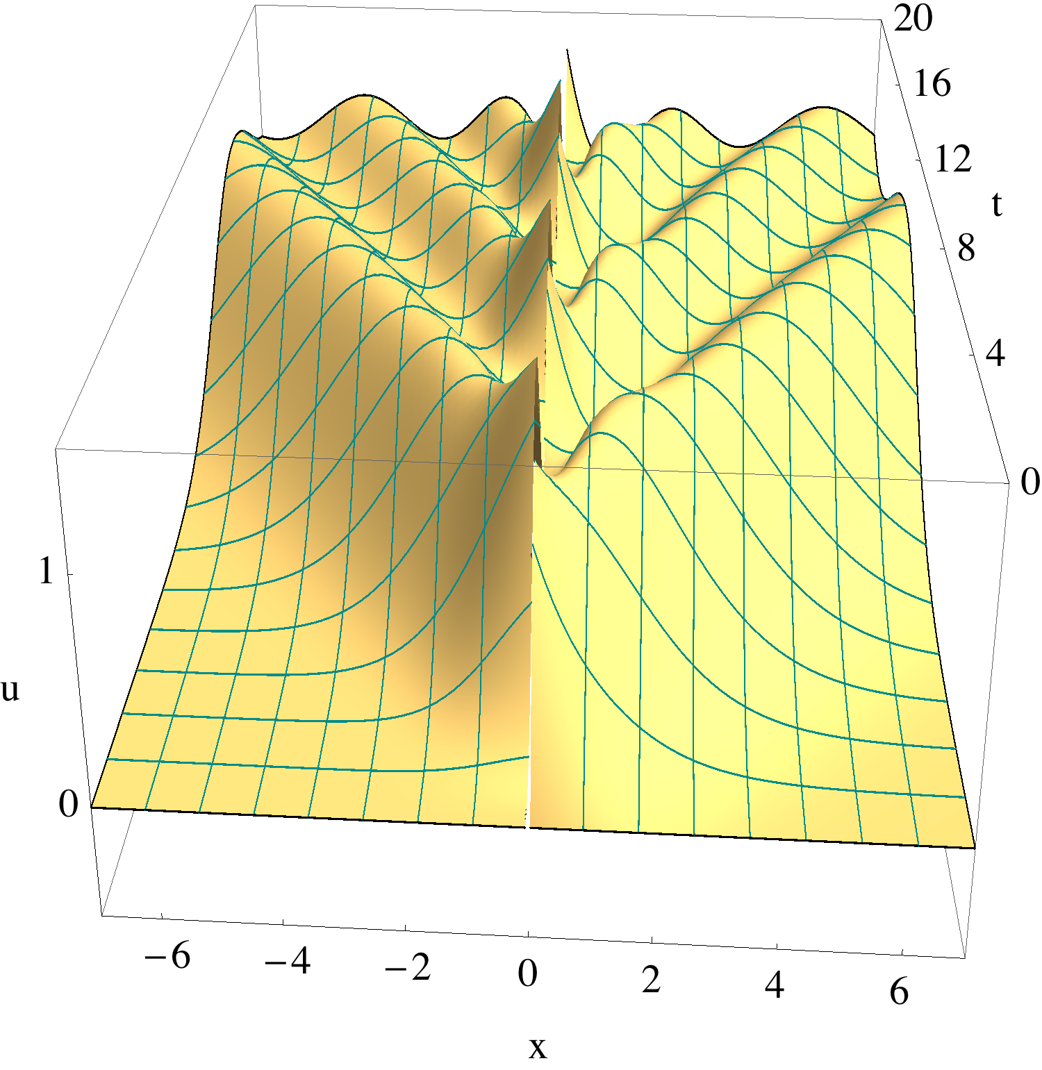
We consider the calculation of the solutions of the homogeneous wave equation using (2.2). Since the governing peridynamic operator is bounded, the functions of that operator in (2.2) can be represented in form of power series in the governing operator. We provide a representation of a class of holomorphic functions of a bounded, self-adjoint operator in Lemma 4.1. We apply this representation to the functions present in the solution of the initial value problem of the homogeneous wave equation in Lemma 4.2. Lemma 4.1 and Lemma 4.2 can be viewed as straightforward applications of the spectral theorems for densely-defined, self-adjoint linear operators in Hilbert spaces. On the other hand, the matrix entries of the governing operator are sums of two commuting operators, a multiple of the identity operator and a convolution. Therefore, power series expansions in terms of the convolution operator turn out to be more useful. For this purpose, the application of the new expansions given in Theorems 4.3, 4.5 and 4.7 proved to be superior; see Examples 5.1 and 5.2. In particular, Corollary 4.6 gives an error estimate for the expansion in Theorem 4.5. This error estimate has been used to plot the solution in Figures 5.1 and 5.2.

Lemma 4.1.

(Holomorphic Functional Calculus) Let $(X,\braket{\,|\,})$ be a non-trivial complex Hilbert space, $A\in L(X,X)$ self-adjoint and $\sigma(A)\subset{\mathbb{R}}$ the (non-empty, compact) spectrum of $A$ . Furthermore, let $R>\|A\|$ and $f:U_{R}(0)\rightarrow{\mathbb{C}}$ be holomorphic. Then, the sequence

\left(\frac{f^{(k)}(0)}{k!}.A^{k}\right)_{k\in{\mathbb{N}}}

is absolutely summable in $L(X,X)$ and

(f|_{{\sigma}(A)})(A)=\sum_{k=0}^{\infty}\frac{f^{(k)}(0)}{k!}.A^{k}\,\,.

Proof.

First, we note that according to Taylor’s theorem, general properties of power series and the compactness of $\sigma(A)$ that

\left(\frac{f^{(k)}(0)}{k!}.z^{k}\right)_{k\in{\mathbb{N}}}

is absolutely summable for every $z\in U_{R}(0)$ as well as, since $\sigma(A)\subset B_{\|A\|}(0)\subset U_{R}(0),$ that the sequence of continuous functions

\left(\,\sum_{k=0}^{n}\frac{f^{(k)}(0)}{k!}.{({\textrm{id}}_{\mathbb{R}}}|_{\sigma(A)})^{n}\right)_{n\in{\mathbb{N}}}

converges uniformly to the continuous function $f|_{{\sigma}(A)}$ . In particular, since $\|A\|<R,$ this implies that the sequence

\left(\frac{f^{(k)}(0)}{k!}.A^{k}\right)_{k\in{\mathbb{N}}}

is absolutely summable in $L(X,X)$ , and it follows from the spectral theorem for bounded self-adjoint operators in Hilbert spaces that

\left(\,\sum_{k=0}^{n}\frac{f^{(k)}(0)}{k!}.{({\textrm{id}}_{\mathbb{R}}}|_{\sigma(A)})^{n}\right)(A)=\sum_{k=0}^{n}\frac{f^{(k)}(0)}{k!}.A^{k}\,\,,

as well as that

(f|_{{\sigma}(A)})(A)=\sum_{k=0}^{\infty}\frac{f^{(k)}(0)}{k!}.A^{k}\,\,.

∎

Lemma 4.2.

(Approximations) Let $(X,\braket{\,|\,})$ be a non-trivial complex Hilbert space, $\sqrt{\phantom{ij}}$ the complex square-root function, with domain ${\mathbb{C}}\setminus((-\infty,0]\times\{0\})$ . $A\in L(X,X)$ self-adjoint and $\sigma(A)\subset{\mathbb{R}}$ the (non-empty, compact) spectrum of $A$ . For every $t\in{\mathbb{R}}$ , the sequences

\left((-1)^{k}\,\frac{t^{2k}}{(2k)!}\,.A^{k}\right)_{k\in{\mathbb{N}}}\,\,,\,\,\left((-1)^{k}\,\frac{t^{2k+1}}{(2k+1)!}\,.A^{k}\right)_{k\in{\mathbb{N}}}

are absolutely summable in $L(X,X)$ and

		$\displaystyle\left[\overline{\cos\left(t\sqrt{\phantom{ij}}\right)}\,\bigg\|_{\sigma(A)}\right]\!(A)=\sum_{k=0}^{\infty}(-1)^{k}\,\frac{t^{2k}}{(2k)!}\,A^{k}\,\,,$
		$\displaystyle\left[\,\overline{\frac{\sin\left(t\sqrt{\phantom{ij}}\right)}{\sqrt{\phantom{ij}}}}\,\bigg\|_{\sigma(A)}\right]\!(A)=\sum_{k=0}^{\infty}(-1)^{k}\,\frac{t^{2k+1}}{(2k+1)!}\,A^{k}\,\,.$

Proof.

We note that for every $t\in{\mathbb{R}}$

		$\displaystyle\cos(t\sqrt{\phantom{ij}}\,):{\mathbb{C}}\setminus((-\infty,0]\times\{0\})\rightarrow{\mathbb{C}}\,\,,\,\,$
		$\displaystyle\cosh(t\sqrt{\phantom{ij}}\circ(-{\textrm{id}}_{\mathbb{C}})\,):{\mathbb{C}}\setminus([0,\infty)\times\{0\})\rightarrow{\mathbb{C}}$

are holomorphic function such that

		$\displaystyle\cos(t\sqrt{z}\,)=\sum_{k=0}^{\infty}(-1)^{k}\,\frac{(t\sqrt{z})^{2k}}{(2k)!}=\sum_{k=0}^{\infty}(-1)^{k}\,\frac{t^{2k}}{(2k)!}\,z^{k}\,\,,$
		$\displaystyle\cosh(t\sqrt{-z}\,)=\sum_{k=0}^{\infty}\frac{(t\sqrt{-z})^{2k}}{(2k)!}=\sum_{k=0}^{\infty}(-1)^{k}\,\frac{t^{2k}}{(2k)!}\,z^{k}$

for every $z\in{\mathbb{C}}\setminus((-\infty,0]\times\{0\})$ and $z\in{\mathbb{C}}\setminus[0,\infty)\times\{0\})$ , respectively. As a consequence, there is a unique extension of $\cos(t\sqrt{\phantom{ij}}\,)$ to an entire holomorphic function $\overline{\cos(t\sqrt{\phantom{ij}}\,)}$ such that

\overline{\cos(t\sqrt{\phantom{ij}}\,)}(z)=\sum_{k=0}^{\infty}(-1)^{k}\,\frac{t^{2k}}{(2k)!}\,z^{k}

for every $z\in{\mathbb{C}}$ . Furthermore,

		$\displaystyle\frac{\sin(t\sqrt{\phantom{ij}}\,)}{\sqrt{\phantom{ij}}}:{\mathbb{C}}\setminus((-\infty,0]\times\{0\})\rightarrow{\mathbb{C}}\,\,,\,\,$
		$\displaystyle\frac{\sinh(t\sqrt{\phantom{ij}}\,)}{\sqrt{\phantom{ij}}}\circ(-{\textrm{id}}_{\mathbb{C}}):{\mathbb{C}}\setminus([0,\infty)\times\{0\})\rightarrow{\mathbb{C}}$

are holomorphic function such that

		$\displaystyle\frac{\sin(t\sqrt{z}\,)}{\sqrt{z}}=\frac{1}{\sqrt{z}}\,\sum_{k=0}^{\infty}(-1)^{k}\,\frac{(t\sqrt{z})^{2k+1}}{(2k+1)!}=\sum_{k=0}^{\infty}(-1)^{k}\,\frac{t^{2k+1}}{(2k+1)!}\,z^{k}\,\,,$
		$\displaystyle\frac{\sinh(t\sqrt{-z}\,)}{\sqrt{-z}}=\frac{1}{\sqrt{-z}}\,\sum_{k=0}^{\infty}\frac{(t\sqrt{-z})^{2k+1}}{(2k+1)!}=\sum_{k=0}^{\infty}(-1)^{k}\,\frac{t^{2k+1}}{(2k+1)!}\,z^{k}$

for every $z\in{\mathbb{C}}\setminus((-\infty,0]\times\{0\})$ and $z\in{\mathbb{C}}\setminus[0,\infty)\times\{0\})$ , respectively. As a consequence, there is a unique extension of $\sin(t\sqrt{\phantom{ij}}\,)/\sqrt{\phantom{ij}}$ to an entire holomorphic function

\overline{\frac{\sin(t\sqrt{\phantom{ij}}\,)}{\sqrt{\phantom{ij}}}}

such that

\overline{\frac{\sin(t\sqrt{\phantom{ij}}\,)}{\sqrt{\phantom{ij}}}}\,(z)=\sum_{k=0}^{\infty}(-1)^{k}\,\frac{t^{2k+1}}{(2k+1)!}\,z^{k}

for every $z\in{\mathbb{C}}$ . In particular, it follows from Lemma 4.1 that the sequences

\left((-1)^{k}\,\frac{t^{2k}}{(2k)!}\,.A^{k}\right)_{k\in{\mathbb{N}}}\,\,,\,\,\left((-1)^{k}\,\frac{t^{2k+1}}{(2k+1)!}\,.A^{k}\right)_{k\in{\mathbb{N}}}

are absolutely summable in $L(X,X)$ and that

	$\displaystyle\left[\cos\left(t\sqrt{\phantom{ij}}\right)\bigg\|_{\sigma(A)}\right]\!(A)$	$\displaystyle=\sum_{k=0}^{\infty}(-1)^{k}\,\frac{t^{2k}}{(2k)!}\,A^{k}\,\,,$
	$\displaystyle\left[\,\overline{\frac{\sin\left(t\sqrt{\phantom{ij}}\right)}{\sqrt{\phantom{ij}}}}\,\bigg\|_{\sigma(A)}\right]\!(A)$	$\displaystyle=\sum_{k=0}^{\infty}(-1)^{k}\,\frac{t^{2k+1}}{(2k+1)!}\,A^{k}\,\,.$

∎

In preparation, we provide the power series expansion related to bounded commuting operators. We expect that the expansion below can be used for large time asymptotic of the solutions of the nonlocal wave equation.

Theorem 4.3.

Let $(X,\braket{\,|\,})$ be a non-trivial complex Hilbert space, $\sqrt{\phantom{ij}}$ the complex square-root function, with domain ${\mathbb{C}}\setminus((-\infty,0]\times\{0\})$ . $A,B\in L(X,X)$ self-adjoint such that $[A,B]=0$ and $\sigma(A),\sigma(A+B)\subset{\mathbb{R}}$ the (non-empty, compact) spectra of $A$ and $A+B$ , respectively. Then

		$\displaystyle\left[\overline{\cos\left(t\sqrt{\phantom{ij}}\right)}\,\bigg\|_{\sigma(A+B)}\right]\!(A+B)$
		$\displaystyle=\sum_{k=0}^{\infty}(-1)^{k}\cdot\frac{t^{2k}}{(2k)!}\,.\left\{\left[{\vphantom{F}}{}_{0}F_{1}\!\!\left(-;k+\frac{1}{2};-\,\frac{t^{2}}{4}\,.{\textrm{i}d}_{\sigma(A)}\right)\right]\!\!(A)\right\}\!B^{k}\,\,,$
		$\displaystyle\left[\,\overline{\frac{\sin\left(t\sqrt{\phantom{ij}}\right)}{\sqrt{\phantom{ij}}}}\,\bigg\|_{\sigma(A+B)}\right]\!(A+B)$
		$\displaystyle=\sum_{k=0}^{\infty}(-1)^{k}\cdot\frac{t^{2k+1}}{(2k+1)!}\,.\left\{\left[{\vphantom{F}}{}_{0}F_{1}\!\!\left(-;k+\frac{3}{2};-\,\frac{t^{2}}{4}\,.{\textrm{i}d}_{\sigma(A)}\right)\right]\!\!(A)\right\}\!B^{k}\,\,,$

where ${\vphantom{F}}{}_{0}F_{1}$ denotes the generalized hypergeometric function, defined as in [51].

Proof.

In a first step, we note for every $t\in{\mathbb{R}}$ that the family

\left((-1)^{k+l}\binom{k+l}{l}\,\frac{t^{2(k+l)}}{[2(k+l)]!}\,A^{k}B^{l}\right)_{(k,l)\in{\mathbb{N}}^{2}}

is absolutely summable in $L(X,X)$ , since for $(k,l)\in{\mathbb{N}}^{2}$

		$\displaystyle\bigg\\|(-1)^{k+l}\binom{k+l}{l}\,\frac{t^{2(k+l)}}{[2(k+l)]!}\,A^{k}B^{l}\bigg\\|\leqslant\frac{t^{2(k+l)}}{[2(k+l)]!}\binom{k+l}{l}\\|A\\|^{k}\\|B\\|^{l}$
		$\displaystyle=\frac{(k+l)!}{l!k![2(k+l)]!}\left(\,t^{2}\\|A\\|\,\right)^{\!k}\left(\,t^{2}\\|B\\|\,\right)^{\!l}\leqslant\frac{1}{k!}\left(\,t^{2}\\|A\\|\,\right)^{\!k}\frac{1}{l!}(\,t^{2}\\|B\\|\,)^{l}$

and hence for every finite subset $S\subset{\mathbb{N}}^{2}$

\displaystyle\sum_{(k,l)\in S}\bigg\|(-1)^{k+l}\binom{k+l}{l}\,\frac{t^{2(k+l)}}{[2(k+l)]!}\,A^{k}B^{l}\bigg\|\leqslant\exp\left(t^{2}\|A\|\right)\exp\left(t^{2}\|B\|\right)\,\,.

Also, we note that the family

\left((-1)^{k+l}\binom{k+l}{l}\,\frac{t^{2(k+l)+1}}{[2(k+l)+1]!}\,A^{k}B^{l}\right)_{(k,l)\in{\mathbb{N}}^{2}}

is absolutely summable in $L(X,X)$ , since for $(k,l)\in{\mathbb{N}}^{2}$

		$\displaystyle\bigg\\|(-1)^{k+l}\binom{k+l}{l}\,\frac{t^{2(k+l)+1}}{[2(k+l)+1]!}\,A^{k}B^{l}\bigg\\|_{2}\leqslant\frac{\|t\|^{2(k+l)+1}}{[2(k+l)+1]!}\binom{k+l}{l}\\|A\\|^{k}\\|B\\|^{l}$
		$\displaystyle=\|t\|\,\frac{(k+l)!}{l!k![2(k+l)+1]!}\left(\,t^{2}\\|A\\|\,\right)^{\!k}\left(\,t^{2}\\|B\\|\,\right)^{\!l}\leqslant\|t\|\,\frac{1}{k!}\left(\,t^{2}\\|A\\|\,\right)^{\!k}\frac{1}{l!}(\,t^{2}\\|B\\|\,)^{l}\,\,,$

leading to

\displaystyle\sum_{(k,l)\in S}\left\|(-1)^{k+l}\binom{k+l}{l}\,\frac{t^{2(k+l)+1}}{[2(k+l)+1]!}\,A^{k}B^{l}\right\|\leqslant|t|\exp\left(t^{2}\|A\|\right)\exp\left(t^{2}\|B\|\right)\,\,,

for every finite subset $S\subset{\mathbb{N}}^{2}$ . Hence, we conclude the following.

		$\displaystyle\sum_{k=0}^{\infty}(-1)^{k}\,\frac{t^{2k}}{(2k)!}\,(A+B)^{k}=\sum_{k=0}^{\infty}\sum_{l=0}^{k}(-1)^{k}\,\frac{t^{2k}}{(2k)!}\,\binom{k}{l}A^{k-l}B^{l}$
		$\displaystyle=\sum_{l=0}^{\infty}\sum_{k=l}^{\infty}(-1)^{k}\,\frac{t^{2k}}{(2k)!}\,\binom{k}{l}A^{k-l}B^{l}=\sum_{l=0}^{\infty}\left[\sum_{k=l}^{\infty}(-1)^{k}\,\binom{k}{l}\frac{t^{2k}}{(2k)!}\,A^{k-l}\right]\!B^{l}$
		$\displaystyle=\sum_{l=0}^{\infty}\left[\sum_{k=0}^{\infty}(-1)^{k+l}\binom{k+l}{l}\,\frac{t^{2(k+l)}}{[2(k+l)]!}\,A^{k}\right]\!B^{l}$
		$\displaystyle=\sum_{l=0}^{\infty}(-1)^{l}t^{2l}\left[\sum_{k=0}^{\infty}(-1)^{k}\binom{k+l}{l}\,\frac{t^{2k}}{[2(k+l)]!}\,A^{k}\right]\!B^{l}$
		$\displaystyle=\sum_{l=0}^{\infty}(-1)^{l}\,t^{2l}\left[\sum_{k=0}^{\infty}\frac{(k+l)!}{[2(k+l)]!\cdot l!}\cdot\frac{1}{k!}\,(-t^{2}A)^{k}\right]\!B^{l}$

In the following, we show the auxiliary result that for every $k,l\in{\mathbb{N}}$ ,

\frac{(k+l)!}{[2(k+l)]!\cdot l!}=2^{-k}\cdot\frac{1}{\prod_{m=0}^{k-1}[2(l+m)+1]}\cdot\frac{1}{(2l)!}

(4.1)

The proof proceeds by induction on $k$ . First, we note that

\frac{l!}{(2l)!\cdot l!}=2^{-0}\cdot\frac{1}{\prod_{m=0}^{-1}[2(l+m)+1]}\cdot\frac{1}{(2l)!}\,\,.

In the following, we assume that (4.1) is true for some $k\in{\mathbb{N}}$ . Then

		$\displaystyle\frac{(k+l+1)!}{[2(k+l+1)]!\cdot l!}=\frac{1}{2}\cdot\frac{1}{2(k+l)+1}\cdot\frac{(k+l)!}{[2(k+l)]!\cdot l!}$
		$\displaystyle=\frac{1}{2}\cdot\frac{1}{2(k+l)+1}\cdot 2^{-k}\cdot\frac{1}{\prod_{m=0}^{k-1}[2(l+m)+1]}\cdot\frac{1}{(2l)!}$
		$\displaystyle=2^{-(k+1)}\cdot\frac{1}{\prod_{m=0}^{k}[2(l+m)+1]}\cdot\frac{1}{(2l)!}\,\,,$

and hence (4.1) is true for $k+1$ . The equality (4.1) implies for every $k,l\in{\mathbb{N}}$ that

		$\displaystyle\frac{(k+l)!}{[2(k+l)]!\cdot l!}=2^{-k}\cdot\frac{1}{\prod_{m=0}^{k-1}[2(l+m)+1]}\cdot\frac{1}{(2l)!}$
		$\displaystyle=4^{-k}\cdot\frac{1}{\prod_{m=0}^{k-1}\left(l+m+\frac{1}{2}\right)}\cdot\frac{1}{(2l)!}=4^{-k}\cdot\frac{1}{(2l)!\left(l+\frac{1}{2}\right)_{k}}$

Hence

		$\displaystyle\sum_{k=0}^{\infty}(-1)^{k}\,\frac{t^{2k}}{(2k)!}\,(A+B)^{k}=\sum_{l=0}^{\infty}(-1)^{l}\,t^{2l}\left[\sum_{k=0}^{\infty}\frac{1}{(2l)!\left(l+\frac{1}{2}\right)_{k}}\cdot\frac{1}{k!}\,\left(-\,\frac{t^{2}}{4}\,.A\right)^{k}\right]\!B^{l}$
		$\displaystyle\sum_{l=0}^{\infty}(-1)^{l}\,\frac{t^{2l}}{(2l)!}\left[\sum_{k=0}^{\infty}\frac{1}{\left(l+\frac{1}{2}\right)_{k}\cdot k!}\cdot\left(-\,\frac{t^{2}}{4}\,.A\right)^{k}\right]\!B^{l}\,\,.$

By definition of the generalized hypergeometric function ${\vphantom{F}}{}_{0}F_{1}$ , for every $l\in{\mathbb{N}}$ , $z\in{\mathbb{C}}$

{\vphantom{F}}{}_{0}F_{1}\!\!\left(-;l+\frac{1}{2};z\right)=\sum_{k=0}^{\infty}\frac{z^{k}}{(l+\frac{1}{2})_{k}\cdot k!}\,\,.

(4.2)

Hence

\displaystyle\sum_{k=0}^{\infty}(-1)^{k}\,\frac{t^{2k}}{(2k)!}\,(A+B)^{k}=\sum_{l=0}^{\infty}(-1)^{l}\cdot\frac{t^{2l}}{(2l)!}\,.\left\{\left[{\vphantom{F}}{}_{0}F_{1}\!\!\left(-;l+\frac{1}{2};-\,\frac{t^{2}}{4}\,.{\textrm{i}d}_{\sigma(A)}\right)\right]\!\!(A)\right\}\!B^{l}\,\,.

Furthermore,

		$\displaystyle\sum_{k=0}^{\infty}(-1)^{k}\,\frac{t^{2k+1}}{(2k+1)!}\,(A+B)^{k}=\sum_{k=0}^{\infty}\sum_{l=0}^{k}(-1)^{k}\,\frac{t^{2k+1}}{(2k+1)!}\,\binom{k}{l}A^{k-l}B^{l}$
		$\displaystyle=\sum_{l=0}^{\infty}\sum_{k=l}^{\infty}(-1)^{k}\,\frac{t^{2k+1}}{(2k+1)!}\,\binom{k}{l}A^{k-l}B^{l}=\sum_{l=0}^{\infty}\left[\sum_{k=l}^{\infty}(-1)^{k}\,\binom{k}{l}\frac{t^{2k+1}}{(2k+1)!}\,A^{k-l}\right]\!B^{l}$
		$\displaystyle=\sum_{l=0}^{\infty}\left[\sum_{k=0}^{\infty}(-1)^{k+l}\binom{k+l}{l}\,\frac{t^{2(k+l)+1}}{[2(k+l)+1]!}\,A^{k}\right]\!B^{l}$
		$\displaystyle=\sum_{l=0}^{\infty}(-1)^{l}t^{2l+1}\left[\sum_{k=0}^{\infty}(-1)^{k}\binom{k+l}{l}\,\frac{t^{2k}}{[2(k+l)+1]!}\,A^{k}\right]\!B^{l}$
		$\displaystyle=t\sum_{l=0}^{\infty}(-1)^{l}\cdot t^{2l}\left[\sum_{k=0}^{\infty}\frac{(k+l)!}{[2(k+l)+1]!\cdot l!}\cdot\frac{1}{k!}\,.\left(-t^{2}A\right)^{k}\right]\!B^{l}\,\,.$

Since for every $k,l\in{\mathbb{N}}$

		$\displaystyle\frac{(k+l)!}{[2(k+l)+1]!\cdot l!}=\frac{1}{2}\cdot\frac{1}{k+l+\frac{1}{2}}\cdot\frac{(k+l)!}{[2(k+l)]!\cdot l!}$
		$\displaystyle=\frac{1}{2}\cdot\frac{1}{k+l+\frac{1}{2}}\cdot 4^{-k}\cdot\frac{1}{(2l)!\left(l+\frac{1}{2}\right)_{k}}=\frac{1}{2}\cdot 4^{-k}\cdot\frac{1}{(2l)!\left(l+\frac{1}{2}\right)\left(l+\frac{3}{2}\right)_{k}}$
		$\displaystyle=4^{-k}\cdot\frac{1}{(2l+1)!\left(l+\frac{3}{2}\right)_{k}}\,\,,$

we conclude that

		$\displaystyle\sum_{k=0}^{\infty}(-1)^{k}\,\frac{t^{2k+1}}{(2k+1)!}\,(A+B)^{k}$
		$\displaystyle=t\sum_{l=0}^{\infty}(-1)^{l}\cdot t^{2l}\left[\sum_{k=0}^{\infty}\frac{1}{(2l+1)!\left(l+\frac{3}{2}\right)_{k}}\cdot\frac{1}{k!}\,.\left(-\,\frac{t^{2}}{4}\,.A\right)^{k}\right]\!B^{l}$
		$\displaystyle=\sum_{l=0}^{\infty}(-1)^{l}\cdot\frac{t^{2l+1}}{(2l+1)!}\left[\sum_{k=0}^{\infty}\frac{1}{\left(l+\frac{3}{2}\right)_{k}\cdot k!}\,.\left(-\,\frac{t^{2}}{4}\,.A\right)^{k}\right]\!B^{l}$
		$\displaystyle=\sum_{l=0}^{\infty}(-1)^{l}\cdot\frac{t^{2l+1}}{(2l+1)!}\,.\left\{\left[{\vphantom{F}}{}_{0}F_{1}\!\!\left(-;l+\frac{3}{2};-\,\frac{t^{2}}{4}\,.{\textrm{i}d}_{\sigma(A)}\right)\right]\!\!(A)\right\}\!B^{l}\,\,.$

∎

The following lemma gives a connection between generalized hypergeometric and spherical Bessel functions.

Lemma 4.4.

For every $k\in{\mathbb{N}}$ and $x>0$

	$\displaystyle\frac{x^{2k}}{(2k)!}\,.\,{\vphantom{F}}_{0}F_{1}\!\!\left(-;k+\frac{1}{2};-\,\frac{x^{2}}{4}\right)$	$\displaystyle=\frac{1}{2^{k}k!}\,x^{k+1}j_{k-1}(x)\,\,,$
	$\displaystyle\frac{x^{2k+1}}{(2k+1)!}\cdot{\vphantom{F}}_{0}F_{1}\left(-;k+\frac{3}{2},-\frac{x^{2}}{4}\right)$	$\displaystyle=\frac{1}{2^{k}k!}\,x^{k+1}j_{k}(\|x\|)\,\,,$

where the spherical Bessel functions $j_{0},j_{1},\dots$ are defined as in [51] and

j_{-1}(x):=\frac{\cos(x)}{x},\quad x>0.

Proof.

We note that for every $\nu\in(0,\infty)$ , $k\in{\mathbb{N}}$ , and $x>0$

	$\displaystyle J_{\nu}(x)$	$\displaystyle:=\left(\frac{x}{2}\right)^{\nu}\sum_{k=0}^{\infty}\frac{(-1)^{k}}{k!\,\Gamma(\nu+k+1)}\left(\frac{x^{2}}{4}\right)^{k}=\frac{1}{\Gamma(\nu+1)}\cdot\left(\frac{x}{2}\right)^{\nu}\sum_{k=0}^{\infty}\frac{(-1)^{k}}{k!\,\frac{\Gamma(\nu+k+1)}{\Gamma(\nu+1)}}\left(\frac{x^{2}}{4}\right)^{k}$
		$\displaystyle\phantom{:}=\frac{1}{\Gamma(\nu+1)}\cdot\left(\frac{x}{2}\right)^{\nu}\sum_{k=0}^{\infty}\frac{(-1)^{k}}{k!\,(\nu+1)_{k}}\left(\frac{x^{2}}{4}\right)^{k}=\frac{1}{\Gamma(\nu+1)}\cdot\left(\frac{x}{2}\right)^{\nu}\cdot{\vphantom{F}}_{0}F_{1}(-;\nu+1,-x^{2}/4)\,\,.$

	$\displaystyle j_{k}(x)$	$\displaystyle:=\sqrt{\frac{\pi}{2x}}\,J_{k+\frac{1}{2}}(x)=\sqrt{\frac{\pi}{2x}}\,\frac{1}{\Gamma(k+\frac{3}{2})}\cdot\left(\frac{x}{2}\right)^{k+\frac{1}{2}}\cdot{\vphantom{F}}_{0}F_{1}(-;k+\frac{3}{2},-x^{2}/4)$
		$\displaystyle\phantom{:}=\frac{\sqrt{\pi}}{2\Gamma(k+\frac{3}{2})}\cdot\left(\frac{x}{2}\right)^{k}\cdot{\vphantom{F}}_{0}F_{1}(-;k+\frac{3}{2},-x^{2}/4)\,\,.$

Hence for every $k\in{\mathbb{N}}$ , $x>0$

{\vphantom{F}}{}_{0}F_{1}(-;k+\frac{3}{2},-x^{2}/4)=\frac{2\Gamma(k+\frac{3}{2})}{\sqrt{\pi}}\left(\frac{x}{2}\right)^{-k}j_{k}(x)=2^{k+1}\left(\frac{1}{2}\right)_{\!k+1}x^{-k}j_{k}(x)

as well as

		$\displaystyle\frac{x^{2k+1}}{(2k+1)!}\,{\vphantom{F}}_{0}F_{1}(-;k+\frac{3}{2},-x^{2}/4)=\frac{x^{2k+1}}{(2k+1)!}\,2^{k+1}\left(\frac{1}{2}\right)_{\!k+1}x^{-k}j_{k}(x)$
		$\displaystyle=\frac{x^{2k+1}}{(2k+1)!}\,2^{k+1}\,2^{-(k+1)}\,\frac{(2k+2)!}{2^{k+1}(k+1)!}x^{-k}j_{k}(x)=\frac{(2k+2)}{2^{k+1}(k+1)!}\,x^{k+1}j_{k}(x)$
		$\displaystyle=\frac{1}{2^{k}k!}\,x^{k+1}j_{k}(x)\,\,.$

Furthermore, for every $k\in{\mathbb{N}}^{*}$ , $x>0$

\frac{x^{2k}}{(2k)!}\,.\,{\vphantom{F}}_{0}F_{1}(-;k+\frac{1}{2};-x^{2}/4)=\frac{x}{2k}\,\frac{1}{2^{k-1}(k-1)!}\,x^{k}j_{k-1}(x)=\frac{1}{2^{k}k!}\,x^{k+1}j_{k-1}(x)\,\,.

(4.3)

Since for $x>0$

		${\vphantom{F}}{}_{0}F_{1}(-;\frac{1}{2},-x^{2}/4)=\sum_{k=0}^{\infty}\frac{1}{\left(\frac{1}{2}\right)_{k}\cdot k!}\cdot\left(-\,\frac{x^{2}}{4}\right)^{k}=\sum_{k=0}^{\infty}\frac{1}{2^{-k}\cdot\frac{(2k)!}{2^{k}\cdot k!}\cdot k!}\cdot\left(-\,\frac{x^{2}}{4}\right)^{k}$
		$\displaystyle=\sum_{k=0}^{\infty}\frac{4^{k}}{(2k)!}\cdot\left(-\,\frac{x^{2}}{4}\right)^{k}=\sum_{k=0}^{\infty}(-1)^{k}\,\frac{x^{2k}}{(2k)!}=\cos(x)\,\,,$

the equality (4.3) is true also for $k=0$ , if we define

j_{-1}(x):=\frac{\cos(x)}{x}\,\,.

∎

Eventually, we have a representation involving two commuting operators, with one of the operators being a multiple of the identity and a general $C$ which is not necessarily a convolution operator.

Theorem 4.5.

Let $(X,\braket{\,|\,})$ be a non-trivial complex Hilbert space, $\sqrt{\phantom{ij}}$ the complex square-root function, with domain ${\mathbb{C}}\setminus((-\infty,0]\times\{0\})$ . $c>0$ , $C\in L(X,X)$ self-adjoint and $\sigma(c-C)\subset{\mathbb{R}}$ the (non-empty, compact) spectrum of $c-C$ . Then for every $t\in{\mathbb{R}}$

		$\displaystyle\left[\overline{\cos\left(t\sqrt{\phantom{ij}}\right)}\,\bigg\|_{\sigma(c-C)}\right]\!(c-C)=\sum_{k=0}^{\infty}\,\frac{1}{2^{k}k!}\,(\sqrt{ct^{2}}\,)^{k+1}j_{k-1}(\sqrt{ct^{2}}\,)\!\left(\frac{1}{c}.C\right)^{\!\!k}\,\,,$
		$\displaystyle\left[\,\overline{\frac{\sin\left(t\sqrt{\phantom{ij}}\right)}{\sqrt{\phantom{ij}}}}\,\bigg\|_{\sigma(c-C)}\right]\!(c-C)=t\sum_{k=0}^{\infty}\,\frac{1}{2^{k}k!}\,(\sqrt{ct^{2}}\,)^{k}j_{k}(\sqrt{ct^{2}}\,)\!\left(\frac{1}{c}.C\right)^{\!\!k}\,\,,$

where the spherical Bessel functions $j_{0},j_{1},\dots$ are defined as in [51] and

j_{-1}(x):=\frac{\cos(x)}{x},\quad x>0

and the members of the sums are defined for $t=0$ by continuous extension.

Proof.

Direct consequence of Theorem 4.3 and Lemma 4.4. ∎

We provide an error estimate of the previous representation.

Corollary 4.6.

(Error Estimates) Let $(X,\braket{\,|\,}),\sqrt{\phantom{ij}},c,C,\sigma(c-C),j_{-1},j_{0},j_{1},\dots$ as in Theorem 4.5 and $N\in{\mathbb{N}}$ . Then for every $t\in{\mathbb{R}}$

		$\displaystyle\left\\|\left[\overline{\cos\left(t\sqrt{\phantom{ij}}\right)}\,\bigg\|_{\sigma(c-C)}\right]\!(c-C)-\sum_{k=0}^{N}\,\frac{1}{2^{k}k!}\,(\sqrt{ct^{2}}\,)^{k+1}j_{k-1}(\sqrt{ct^{2}}\,)\!\left(\frac{1}{c}.C\right)^{\!\!k}\right\\|$
		$\displaystyle\leqslant\frac{\pi}{N!}\,\min\left\{1,\left(\!\frac{t^{2}\\|C\\|}{4}\!\right)^{\!\!N+1}\right\}e^{\,t^{2}\\|C\\|/4}\,\,,$
		$\displaystyle\left\\|\left[\,\overline{\frac{\sin\left(t\sqrt{\phantom{ij}}\right)}{\sqrt{\phantom{ij}}}}\,\bigg\|_{\sigma(c-C)}\right]\!(c-C)-t\sum_{k=0}^{\infty}\,\frac{1}{2^{k}k!}\,(\sqrt{ct^{2}}\,)^{k}j_{k}(\sqrt{ct^{2}}\,)\!\left(\frac{1}{c}.C\right)^{\!\!k}\right\\|$
		$\displaystyle\leqslant\frac{\pi}{2(N+1)!}\,\|t\|\,\min\left\{1,\left(\!\frac{t^{2}\\|C\\|}{4}\!\right)^{\!\!N+1}\right\}e^{\,t^{2}\\|C\\|/4}\,\,.$

Proof.

As a consequence of Theorem 4.5, for $t\in{\mathbb{R}}$

		$\displaystyle\left\\|\left[\overline{\cos\left(t\sqrt{\phantom{ij}}\right)}\,\bigg\|_{\sigma(c-C)}\right]\!(c-C)-\sum_{k=0}^{N}\,\frac{1}{2^{k}k!}\,(\sqrt{ct^{2}}\,)^{k+1}j_{k-1}(\sqrt{ct^{2}}\,)\!\left(\frac{1}{c}.C\right)^{\!\!k}\right\\|$
		$\displaystyle\leqslant\sum_{k=N+1}^{\infty}\,\frac{1}{2^{k}k!}\,(\sqrt{ct^{2}}\,)^{k+1}\|\,j_{k-1}(\sqrt{ct^{2}}\,)\|\left(\!\frac{\\|C\\|}{c}\!\right)^{\!\!k}$
		$\displaystyle\leqslant\sum_{k=N+1}^{\infty}\,\frac{1}{2^{k}k!}\,(\sqrt{ct^{2}}\,)^{k+1}\,\pi\,\frac{(\sqrt{ct^{2}}\,)^{k-1}}{2^{k}(k-1)!}\left(\!\frac{\\|C\\|}{c}\!\right)^{\!\!k}$
		$\displaystyle=\pi\sum_{k=N+1}^{\infty}\,\frac{1}{k!(k-1)!}\left(\!\frac{t^{2}\\|C\\|}{4}\!\right)^{\!\!k}\leqslant\frac{\pi}{N!}\sum_{k=N+1}^{\infty}\,\frac{1}{k!}\left(\!\frac{t^{2}\\|C\\|}{4}\!\right)^{\!\!k}\,\,,$

where the integral representation DLMF 10.54.1 of [51] (http://dlmf.nist.gov/10.54) for spherical Bessel functions has been used. Since

		$\displaystyle\sum_{k=N+1}^{\infty}\,\frac{1}{k!}\left(\!\frac{t^{2}\\|C\\|}{4}\!\right)^{\!\!k}=\left(\!\frac{t^{2}\\|C\\|}{4}\!\right)^{\!\!N+1}\sum_{k=N+1}^{\infty}\,\frac{1}{k!}\left(\!\frac{t^{2}\\|C\\|}{4}\!\right)^{\!\!k-N-1}$
		$\displaystyle\leqslant\left(\!\frac{t^{2}\\|C\\|}{4}\!\right)^{\!\!N+1}\sum_{k=N+1}^{\infty}\,\frac{1}{(k-N-1)!}\left(\!\frac{t^{2}\\|C\\|}{4}\!\right)^{\!\!k-N-1}\leqslant\left(\!\frac{t^{2}\\|C\\|}{4}\!\right)^{\!\!N+1}e^{\,t^{2}\\|C\\|/4}\,\,,$

this implies that

		$\displaystyle\left\\|\left[\overline{\cos\left(t\sqrt{\phantom{ij}}\right)}\,\bigg\|_{\sigma(c-C)}\right]\!(c-C)-\sum_{k=0}^{N}\,\frac{1}{2^{k}k!}\,(\sqrt{ct^{2}}\,)^{k+1}j_{k-1}(\sqrt{ct^{2}}\,)\!\left(\frac{1}{c}.C\right)^{\!\!k}\right\\|$
		$\displaystyle\leqslant\frac{\pi}{N!}\,\min\left\{1,\left(\!\frac{t^{2}\\|C\\|}{4}\!\right)^{\!\!N+1}\right\}e^{\,t^{2}\\|C\\|/4}\,\,.$

Furthermore,

		$\displaystyle\left\\|\left[\,\overline{\frac{\sin\left(t\sqrt{\phantom{ij}}\right)}{\sqrt{\phantom{ij}}}}\,\bigg\|_{\sigma(c-C)}\right]\!(c-C)-t\sum_{k=0}^{N}\,\frac{1}{2^{k}k!}\,(\sqrt{ct^{2}}\,)^{k}j_{k}(\sqrt{ct^{2}}\,)\!\left(\frac{1}{c}.C\right)^{\!\!k}\right\\|$
		$\displaystyle\leqslant\|t\|\sum_{k=N+1}^{\infty}\,\frac{1}{2^{k}k!}\,(\sqrt{ct^{2}}\,)^{k}\|\,j_{k}(\sqrt{ct^{2}}\,)\|\left(\!\frac{\\|C\\|}{c}\!\right)^{\!\!k}$
		$\displaystyle\leqslant\|t\|\sum_{k=N+1}^{\infty}\,\frac{1}{2^{k}k!}\,(\sqrt{ct^{2}}\,)^{k}\,\pi\,\frac{(\sqrt{ct^{2}}\,)^{k}}{2^{k+1}k!}\left(\!\frac{\\|C\\|}{c}\!\right)^{\!\!k}$
		$\displaystyle=\frac{\pi}{2}\,\|t\|\sum_{k=N+1}^{\infty}\,\frac{1}{(k!)^{2}}\left(\!\frac{t^{2}\\|C\\|}{4}\!\right)^{\!\!k}\leqslant\frac{\pi}{2(N+1)!}\,\|t\|\sum_{k=N+1}^{\infty}\,\frac{1}{k!}\left(\!\frac{t^{2}\\|C\\|}{4}\!\right)^{\!\!k}$
		$\displaystyle\leqslant\frac{\pi}{2(N+1)!}\,\|t\|\,\min\left\{1,\left(\!\frac{t^{2}\\|C\\|}{4}\!\right)^{\!\!N+1}\right\}e^{\,t^{2}\\|C\\|/4}\,\,.$

∎

Application of Theorem 4.5 to the special case of $A_{C}$ gives the following.

Theorem 4.7.

Let $n\in{\mathbb{N}}^{*}$ , $\rho>0$ , $C\in L^{1}({\mathbb{R}}^{n})$ be even such that

c:=\int_{{\mathbb{R}}^{n}}C\,dv^{n}>0

and $A_{C}$ as in Lemma 3.2. Then for $t\in{\mathbb{R}}$

		$\displaystyle\left[\overline{\cos\left(t\sqrt{\phantom{ij}}\right)}\,\bigg\|_{\sigma(A_{C})}\right]\!(A_{C})f=\sum_{k=0}^{\infty}\frac{1}{2^{k}k!}(\sqrt{ct^{2}/\rho}\,)^{k+1}j_{k-1}(\sqrt{ct^{2}/\rho}\,)\,c^{-k}.C^{k}*f\,\,,$
		$\displaystyle\left[\,\overline{\frac{\sin\left(t\sqrt{\phantom{ij}}\right)}{\sqrt{\phantom{ij}}}}\,\bigg\|_{\sigma(A_{C})}\right]\!(A_{C})f=t\sum_{k=0}^{\infty}\frac{1}{2^{k}k!}(\sqrt{ct^{2}/\rho}\,)^{k}j_{k}(\sqrt{ct^{2}/\rho}\,)\,c^{-k}.C^{k}*f\,\,,$		(4.4)

for every $f\in L^{2}_{\mathbb{C}}({\mathbb{R}}^{n})$ , where the spherical Bessel functions $j_{0},j_{1},\dots$ are defined as in [51],

j_{-1}(z):=\frac{\cos(z)}{z},\quad z\in{\mathbb{C}}^{*},

and the members of the sums are defined for $t=0$ by continuous extension.

Proof.

The statement is a direct consequence of Theorems 3.2 and 4.5. ∎

5 Examples

Refer to caption — (a) Generalized solution $u$ to the classical (local) wave equation with initial data $u(0,x)=1/(1+x^{2})$ and $(\partial u/\partial t)(0,x)=0,~x\in{\mathbb{R}}$ .

We apply the apparatus we have constructed of the previous section on an example that involves a micromodulus and input function both of which are normal distributions with mean value zero and standard deviation $\sigma$ and $\sigma_{d}$ , respectively.

Example 5.1.

For $\rho,\sigma,\sigma_{d},a>0$ , we define $C_{\sigma}\in L^{1}({\mathbb{R}})$ and $f\in L^{2}_{\mathbb{C}}({\mathbb{R}})$ by

\displaystyle C_{\sigma}:=\frac{a}{\sqrt{2\pi}\,\sigma}\,e^{-[1/(2\sigma^{2})].{\mathrm{id}}_{\mathbb{R}}^{2}}\,\,,\,\,f:=\frac{1}{\sqrt{2\pi}\sigma_{d}}\,e^{-[1/(2\sigma_{d}^{2})].{\mathrm{id}}_{\mathbb{R}}^{2}}\,\,.

Then for $k\in{\mathbb{N}}^{*}$

		$\displaystyle F_{1}C_{\sigma}=ae^{-(\sigma^{2}/2).{\mathrm{id}}_{\mathbb{R}}^{2}}\,\,,\,\,F_{1}C_{\sigma}^{k}=(F_{1}C_{\sigma})^{k}=a^{k}e^{-k(\sigma^{2}/2).{\mathrm{id}}_{\mathbb{R}}^{2}}\,\,,$
		$\displaystyle F_{2}(C_{\sigma}^{k}*f)=(F_{1}C_{\sigma}^{k})\cdot F_{2}f=\frac{a^{k}}{\sqrt{2\pi}}\,e^{-k(\sigma^{2}/2).{\mathrm{id}}_{\mathbb{R}}^{2}}\cdot e^{-(\sigma_{d}^{2}/2).{\mathrm{id}}_{\mathbb{R}}^{2}}$
		$\displaystyle=\frac{a^{k}}{\sqrt{2\pi}}\,e^{-[(k\sigma^{2}+\sigma_{d}^{2})/2].{\mathrm{id}}_{\mathbb{R}}^{2}}=\frac{1}{\sqrt{2\pi}}\,F_{1}\frac{a^{k}}{\sqrt{2\pi}\sqrt{k\sigma^{2}+\sigma_{d}^{2}}}\,e^{-\{1/[2(k\sigma^{2}+\sigma_{d}^{2})]\}.{\mathrm{id}}_{\mathbb{R}}^{2}}$
		$\displaystyle=F_{2}\frac{a^{k}}{\sqrt{2\pi}\sqrt{k\sigma^{2}+\sigma_{d}^{2}}}\,e^{-\{1/[2(k\sigma^{2}+\sigma_{d}^{2})]\}.{\mathrm{id}}_{\mathbb{R}}^{2}}$

and hence

C_{\sigma}^{k}*f=\frac{a^{k}}{\sqrt{2\pi}\sqrt{k\sigma^{2}+\sigma_{d}^{2}}}\,e^{-\{1/[2(k\sigma^{2}+\sigma_{d}^{2})]\}.{\mathrm{id}}_{\mathbb{R}}^{2}}\,\,.

Since

c=\int_{\mathbb{R}}C_{\sigma}\,dv^{1}=a>0\,\,,

we conclude from Theorem 4.7 that for $t\in{\mathbb{R}}$

	$\displaystyle\left[\overline{\cos\left(t\sqrt{\phantom{ij}}\right)}\,\bigg\|_{\sigma(A_{C})}\right]\!(A_{C})f$
	$\displaystyle=\sum_{k=0}^{\infty}\frac{1}{2^{k}k!}(\sqrt{at^{2}/\rho}\,)^{k+1}j_{k-1}(\sqrt{at^{2}/\rho}\,)\,\frac{1}{\sqrt{2\pi}\sqrt{k\sigma^{2}+\sigma_{d}^{2}}}\,e^{-\{1/[2(k\sigma^{2}+\sigma_{d}^{2})]\}.{\mathrm{id}}_{\mathbb{R}}^{2}}\,\,,$
	$\displaystyle\left[\,\overline{\frac{\sin\left(t\sqrt{\phantom{ij}}\right)}{\sqrt{\phantom{ij}}}}\,\bigg\|_{\sigma(A_{C})}\right]\!(A_{C})f$
	$\displaystyle=t\sum_{k=0}^{\infty}\frac{1}{2^{k}k!}(\sqrt{at^{2}/\rho}\,)^{k}j_{k}(\sqrt{at^{2}/\rho}\,)\,\frac{1}{\sqrt{2\pi}\sqrt{k\sigma^{2}+\sigma_{d}^{2}}}\,e^{-\{1/[2(k\sigma^{2}+\sigma_{d}^{2})]\}.{\mathrm{id}}_{\mathbb{R}}^{2}}\,\,,$		(5.1)

where $A_{C}$ is as in Lemma 3.2.

We depict and compare the solutions of the classical and nonlocal wave equations in Figures 5.1 and 5.2. In the classical case, as expected, we observe the propagation of waves along characteristics; see Figures 1(a) and 1(c) for vanishing initial velocity and displacement, respectively. In the nonlocal case, we observe repeated separation of waves and an oscillation at the center of the initial pulse; see Figures 1(b) and 1(d) for vanishing initial velocity and displacement, respectively.

We study the propagation of discontinuity in the data for classical and nonlocal wave equations in the following example.

Example 5.2.

As in the previous example, for $\rho,\sigma,a,b,\varepsilon>0$ , we define $C_{\sigma}\in L^{1}({\mathbb{R}})$ by

\displaystyle C_{\sigma}:=\frac{a}{\sqrt{2\pi}\,\sigma}\,e^{-[1/(2\sigma^{2})].{\mathrm{id}}_{\mathbb{R}}^{2}}\,\,.

Then

F_{1}C_{\sigma}=ae^{-(\sigma^{2}/2).{\mathrm{id}}_{\mathbb{R}}^{2}}\,\,,

and for $k\in{\mathbb{N}}^{*}$ ,

F_{1}C_{\sigma}^{k}=(F_{1}C_{\sigma})^{k}=a^{k}e^{-k(\sigma^{2}/2).{\mathrm{id}}_{\mathbb{R}}^{2}}=F_{1}\frac{a^{k}}{\sqrt{2\pi k}\,\sigma}\,e^{-[1/(2k\sigma^{2})].{\mathrm{id}}_{\mathbb{R}}^{2}}\,\,,

and hence

C_{\sigma}^{k}=\frac{a^{k}}{\sqrt{2\pi}\sqrt{k\sigma^{2}}}\,e^{-[1/(2k\sigma^{2})].{\mathrm{id}}_{\mathbb{R}}^{2}}\,\,.

Furthermore, we define $f\in L^{2}_{\mathbb{C}}({\mathbb{R}})$ by

\displaystyle f:=b\,e^{-\varepsilon.{\mathrm{id}}_{\mathbb{R}}}\cdot\chi_{{}_{[0,\infty)}}\,\,.

Then for $x\in{\mathbb{R}}$ ,

		$\displaystyle(C_{\sigma}^{k}*f)(x)=\frac{a^{k}b}{\sqrt{2\pi}\sqrt{k\sigma^{2}}}\,\int_{0}^{\infty}e^{-[(x-y)^{2}/(2k\sigma^{2})]}\cdot e^{-\varepsilon y}\,dy$
		$\displaystyle=\frac{2a^{k}b}{\pi}\,e^{\left(\frac{\varepsilon\sigma}{2}\sqrt{2k}\right)^{2}}\,e^{-\varepsilon x}\,\mathrm{erfc}\!\left(\frac{\varepsilon\sigma}{2}\sqrt{2k}-\frac{x}{\sigma\sqrt{2k}}\right)\,\,,$

where $\mathrm{erfc}$ denotes the error function defined according to DLMF [51]. We note for $x\in{\mathbb{R}}$ that

\lim_{k\rightarrow 0}\frac{a^{k}b}{2}\,e^{\left(\frac{\varepsilon\sigma}{2}\sqrt{2k}\right)^{2}}\,e^{-\varepsilon x}\,\mathrm{erfc}\!\left(\frac{\varepsilon\sigma}{2}\sqrt{2k}-\frac{x}{\sigma\sqrt{2k}}\right)=\begin{cases}0&\text{if $x<0$}\\ \frac{b}{2}&\text{if $x=0$}\\ be^{-\varepsilon x}&\text{if $x>0$}\end{cases}\,\,.

Since

c=\int_{\mathbb{R}}C_{\sigma}\,dv^{1}=a>0\,\,,

we conclude from Theorem 4.7 that for $t\in{\mathbb{R}}$

		$\displaystyle\left[\overline{\cos\left(t\sqrt{\phantom{ij}}\right)}\,\bigg\|_{\sigma(A_{C})}\right]\!(A_{C})f=\sum_{k=0}^{\infty}\frac{1}{2^{k}k!}(\sqrt{at^{2}/\rho}\,)^{k+1}j_{k-1}(\sqrt{at^{2}/\rho}\,)\,f_{k}\,\,,$
		$\displaystyle\left[\,\overline{\frac{\sin\left(t\sqrt{\phantom{ij}}\right)}{\sqrt{\phantom{ij}}}}\,\bigg\|_{\sigma(A_{C})}\right]\!(A_{C})f=t\sum_{k=0}^{\infty}\frac{1}{2^{k}k!}(\sqrt{at^{2}/\rho}\,)^{k}j_{k}(\sqrt{at^{2}/\rho}\,)\,f_{k}\,\,,$		(5.2)

where

	$\displaystyle f_{0}$	$\displaystyle:=b\,e^{-\varepsilon.{\mathrm{id}}_{\mathbb{R}}}\cdot\chi_{{}_{[0,\infty)}}\,\,,$
	$\displaystyle f_{k}(x)$	$\displaystyle:=\frac{2b}{\pi}\,e^{\left(\frac{\varepsilon\sigma}{2}\sqrt{2k}\right)^{2}}\,e^{-\varepsilon x}\,\mathrm{erfc}\!\left(\frac{\varepsilon\sigma}{2}\sqrt{2k}-\frac{x}{\sigma\sqrt{2k}}\right)$
		$\displaystyle\,\,=\frac{b}{\sqrt{2\pi}\sqrt{k\sigma^{2}}}\,e^{-\varepsilon x}\int_{-\infty}^{x}e^{-u^{2}/(2k\sigma^{2})}\cdot e^{\varepsilon u}\,du$

for every $x\in{\mathbb{R}}$ and $k\in{\mathbb{N}}^{*}$ , and where $A_{C}$ is as in Lemma 3.2.

In the classical wave equation, as expected, discontinuities propagate along the characteristics; see Figures 2(a) and 2(c) for vanishing initial velocity and displacement, respectively. On the other hand, in the nonlocal case, the discontinuity remains in the same place for all time; see Figures 2(b) and 2(d) for vanishing initial velocity and displacement, respectively. This confirms the results given in [69].

6 Conclusion

Our result that the governing operator is a bounded function of the classical local operator for scalar-valued functions should be generalizable to vector-valued case. Our notable result that the governing operator $A_{C}$ of the peridynamic wave equation is a bounded function of the classical governing operator has far reaching consequences. It enables the comparison of peridynamic solutions to those of classical elasticity. The remarkable implication is that it opens the possibly of defining peridynamic-type operators on bounded domains as functions of the corresponding classical operator. Since the classical operator is defined through local boundary conditions, the functions inherit this knowledge. This observation opens a gateway to incorporate local boundary conditions into nonlocal theories, which has vital implications for numerical treatment of nonlocal problems. This is the subject of our companion paper [2].

We expect that the expansions in Theorems 4.3 and 4.5 can be used for obtaining the large time asymptotic of solutions of the nonlocal wave equation. In the classical case, as expected, we observe the propagation of waves along characteristics. In the nonlocal case, we observe oscillatory recurrent wave separation. We think that this phenomenon is worth investigating. On the other hand, we observe that discontinuity remains stationary in the nonlocal case, whereas, it is well-known that discontinuities propagate along characteristics. We hold that this fundamentally difference is one of the most distinguishing feature of PD. In conclusion, we believe that we added valuable tools to the of arsenal of methods to analyze nonlocal problems.

Appendix A Some Proofs from Section 2

A.1 Instability of Solutions

We give a proof of Theorem 2.3.

Proof.

Since $\sigma(A)$ is bounded from below, we can define

\lambda_{0}:=\inf\{\lambda\in\sigma(A)\}\,\,.

Furthermore, since $\sigma(A)$ is closed, $\lambda_{0}\in\sigma(A)$ and since

\sigma(A)\cap(-\infty,0)\neq\emptyset\,\,,

we conclude that $\lambda_{0}<0$ . Furthermore, let $f\in C({\mathbb{R}},{\mathbb{R}})$ such that $f|_{[0,\infty)}$ is bounded and such that $f|_{(-\infty,0]}$ is positive and decreasing. In particular, this implies that $f|_{\sigma(A)}\in U^{s}(\sigma(A))$ and also that $f^{2}|_{(-\infty,0]}$ is positive and decreasing. Furthermore, let $0<\varepsilon<|\lambda_{0}|$ . Then there is $\xi\in D(A)$ such that

\eta:=(\chi_{{}_{[\lambda_{0},\lambda_{0}+\varepsilon]}}|_{\sigma(A)})(A)\xi\neq 0_{X}\,\,.

Otherwise, since $D(A)$ is in particular dense in $X$ ,

(\chi_{{}_{[\lambda_{0},\lambda_{0}+\varepsilon]}}|_{\sigma(A)})(A)=0_{L(X,X)}\,\,,

in contradiction to the fact that $\lambda_{0}\in\sigma(A)$ . In particular, since

(\chi_{{}_{[\lambda_{0},\lambda_{0}+\varepsilon]}}|_{\sigma(A)})(A)

and $A$ commute, it follows that $\eta\in D(A)$ .

Furthermore,

		$\displaystyle\\|(f\|_{\sigma(A)})(A)\eta\\|^{2}=\braket{(f\|{}_{\sigma(A)})(A)\eta\|(f\|_{\sigma(A)})(A)\eta}=\braket{\eta\|(f\|{}_{\sigma(A)})^{2}(A)\eta}$
		$\displaystyle=\braket{\xi\|(\chi_{{}_{[\lambda_{0},\lambda_{0}+\varepsilon]}}\|{}_{\sigma(A)})(A)(f\|_{\sigma(A)})^{2}(A)\xi}=\int_{\sigma(A)}\chi_{{}_{[\lambda_{0},\lambda_{0}+\varepsilon]}}\cdot f^{2}\,d\psi_{\xi}$
		$\displaystyle\geqslant\int_{\sigma(A)}\chi_{{}_{[\lambda_{0},\lambda_{0}+\varepsilon]}}\cdot[f(\lambda_{0}+\varepsilon)]^{2}\,d\psi_{\xi}=[f(\lambda_{0}+\varepsilon)]^{2}\int_{\sigma(A)}\chi_{{}_{[\lambda_{0},\lambda_{0}+\varepsilon]}}\,d\psi_{\xi}$
		$\displaystyle=[f(\lambda_{0}+\varepsilon)]^{2}\cdot\\|\eta\\|^{2}.$

In particular, we conclude that

\displaystyle\left\|\left[\overline{\cos\left(t\sqrt{\phantom{ij}}\right)}\,\bigg|_{\sigma(A)}\right]\!(A)\eta\right\|\geqslant\cosh(t\sqrt{|\lambda_{0}+\varepsilon|}\,)\cdot\|\eta\|

for all $t\in{\mathbb{R}}$ . Since $\varepsilon$ is otherwise arbitrary, the latter implies that

\displaystyle\left\|\left[\overline{\cos\left(t\sqrt{\phantom{ij}}\right)}\,\bigg|_{\sigma(A)}\right]\!(A)\eta\right\|\geqslant\cosh(t\sqrt{|\lambda_{0}|}\,)\cdot\|\eta\|\geqslant\frac{1}{2}\,e^{t\sqrt{|\lambda_{0}|}}\cdot\|\eta\|.

∎

A.2 Solutions of Inhomogeneous Wave Equations

We give a proof of Theorem 2.5.

Proof.

In a first step, we note for $\lambda>0$ that

		$\displaystyle\overline{\frac{\sin\left((t-\tau)\sqrt{\phantom{ij}}\right)}{\sqrt{\phantom{ij}}}}\,(\lambda)=\frac{\sin[(t-\tau)\sqrt{\lambda}\,]}{\sqrt{\lambda}}$
		$\displaystyle=\frac{\sin(t\sqrt{\lambda}\,)}{\sqrt{\lambda}}\,\cos(\tau\sqrt{\lambda}\,)-\cos(t\sqrt{\lambda}\,)\,\frac{\sin(\tau\sqrt{\lambda}\,)}{\sqrt{\lambda}}$
		$\displaystyle=\overline{\frac{\sin\left(t\sqrt{\phantom{ij}}\right)}{\sqrt{\phantom{ij}}}}\,(\lambda)\cdot\overline{\cos\left(\tau\sqrt{\phantom{ij}}\right)}\,(\lambda)-\overline{\cos\left(t\sqrt{\phantom{ij}}\right)}\,(\lambda)\cdot\overline{\frac{\sin\left(\tau\sqrt{\phantom{ij}}\right)}{\sqrt{\phantom{ij}}}}\,(\lambda)\,\,.$

Since

\overline{\frac{\sin\left((t-\tau)\sqrt{\phantom{ij}}\right)}{\sqrt{\phantom{ij}}}}\,\,,\,\,\overline{\frac{\sin\left(t\sqrt{\phantom{ij}}\right)}{\sqrt{\phantom{ij}}}}\,\,,\,\,\overline{\cos\left(\tau\sqrt{\phantom{ij}}\right)}\,\,,\,\,\overline{\cos\left(t\sqrt{\phantom{ij}}\right)}\,\,,\,\,\overline{\frac{\sin\left(\tau\sqrt{\phantom{ij}}\right)}{\sqrt{\phantom{ij}}}}\,\,,

are entire functions, this implies that

		$\displaystyle\overline{\frac{\sin\left((t-\tau)\sqrt{\phantom{ij}}\right)}{\sqrt{\phantom{ij}}}}\,(\lambda)$
		$\displaystyle=\overline{\frac{\sin\left(t\sqrt{\phantom{ij}}\right)}{\sqrt{\phantom{ij}}}}\,(\lambda)\cdot\overline{\cos\left(\tau\sqrt{\phantom{ij}}\right)}\,(\lambda)-\overline{\cos\left(t\sqrt{\phantom{ij}}\right)}\,(\lambda)\cdot\overline{\frac{\sin\left(\tau\sqrt{\phantom{ij}}\right)}{\sqrt{\phantom{ij}}}}\,(\lambda)\,\,,$

for every $\lambda\in{\mathbb{C}}$ and hence, by application of the spectral theorem for densely-defined, self-adjoint linear operators in Hilbert spaces, that

		$\displaystyle\left[\,\overline{\frac{\sin\left((t-\tau)\sqrt{\phantom{ij}}\right)}{\sqrt{\phantom{ij}}}}\,\bigg\|_{\sigma(A)}\!\right]\!(A)f(\tau)$
		$\displaystyle=\left\{\left[\,\overline{\frac{\sin\left(t\sqrt{\phantom{ij}}\right)}{\sqrt{\phantom{ij}}}}\,\bigg\|_{\sigma(A)}\!\right]\!(A)\left[\overline{\cos\left(\tau\sqrt{\phantom{ij}}\right)}\,\bigg\|_{\sigma(A)}\!\right]\!(A)\right.$
		$\displaystyle\quad\quad-\left.\left[\overline{\cos\left(t\sqrt{\phantom{ij}}\right)}\,(\lambda)\,\bigg\|_{\sigma(A)}\!\right]\!(A)\left[\overline{\frac{\sin\left(\tau\sqrt{\phantom{ij}}\right)}{\sqrt{\phantom{ij}}}}\,\bigg\|_{\sigma(A)}\!\right]\!(A)\right\}f(\tau)$
		$\displaystyle=b(t)a(\tau)f(\tau)-a(t)b(\tau)f(\tau)$

for all $t,\tau\in{\mathbb{R}}$ , where $a,b:{\mathbb{R}}\rightarrow L(X,X)$ are defined by

\displaystyle a(t):=\left[\overline{\cos\left(t\sqrt{\phantom{ij}}\right)}\,(\lambda)\,\bigg|_{\sigma(A)}\!\right]\!(A)\,\,,\,\,b(t):=\left[\,\overline{\frac{\sin\left(t\sqrt{\phantom{ij}}\right)}{\sqrt{\phantom{ij}}}}\,\bigg|_{\sigma(A)}\!\right]\!(A)\,\,,

for every $t\in{\mathbb{R}}$ . In the following, for $\xi\in D(A)$ , we are going to use that the maps

\displaystyle(\,{\mathbb{R}}\rightarrow X,t\mapsto a(t)\xi\,)\,\,\,\,\text{and}\,\,\,\,(\,{\mathbb{R}}\rightarrow X,t\mapsto b(t)\xi\,)

are differentiable with derivatives

\displaystyle(\,{\mathbb{R}}\rightarrow X,t\mapsto-b(t)A\xi\,)\,\,\,\,\text{and}\,\,\,\,(\,{\mathbb{R}}\rightarrow X,t\mapsto a(t)\xi\,)\,\,,

respectively. We note that, as a consequence of the spectral theorem for densely-defined, self-adjoint linear operators in Hilbert spaces, that $a$ , $b$ are strongly continuous and that

a(t)D(A)\subset D(A)\,\,,\,\,b(t)D(A)\subset D(A)\,\,,

for every $t\in{\mathbb{R}}$ . Also for every $k\in U^{s}_{\mathbb{C}}(\sigma(A))$ , $k(A)D(A)\subset D(A)$ and for $\xi\in D(A)$

\|k(A)\xi\|_{A}^{2}=\|k(A)\xi\|^{2}+\|Ak(A)\xi\|^{2}=\|k(A)\xi\|^{2}+\|k(A)A\xi\|^{2}\,\,\left[\,\leqslant\|k(A)\|_{\text{Op}}^{2}\cdot\|\xi\|_{A}^{2}\,\right]\,\,.

Hence $a,b$ induce strongly continuous maps from ${\mathbb{R}}$ to $X_{A}$ , which we indicate with the same symbols, and where $X_{\!A}:=(D(A),\|\,\,\|_{A})$ . In addition, we note that the inclusion $\iota$ of $X_{A}$ into $X$ is continuous. In the next step, we observe for a strongly continuous $c:{\mathbb{R}}\rightarrow L(X_{\!A},X_{\!A})$ and a continuous $g:{\mathbb{R}}\rightarrow X_{\!A}$ that

		$\displaystyle\\|c(t+h)g(t+h)-c(t)g(t)\\|_{A}$
		$\displaystyle=\\|c(t+h)g(t+h)-c(t+h)g(t)+c(t+h)g(t)-c(t)g(t)\\|_{A}$
		$\displaystyle=\\|c(t+h)[g(t+h)-g(t)]_{A}+[c(t+h)-c(t)]g(t)\\|_{A}$
		$\displaystyle\leqslant\\|c(t+h)\\|\cdot\\|g(t+h)-g(t)\\|_{A}+\\|c(t+h)g(t)-c(t)g(t)\\|_{A}$

and hence that $({\mathbb{R}}\rightarrow X_{\!A},t\mapsto c(t)g(t))$ is continuous as well as that

\displaystyle\left({\mathbb{R}}\rightarrow X_{\!A},t\mapsto\int^{A}_{I_{t}}c(\tau)g(\tau)d\tau\right)\,\,,

where $\int^{A}$ denotes weak integration in $X_{\!A}$ , is differentiable with derivative

({\mathbb{R}}\rightarrow X_{\!A},t\mapsto c(t)g(t))\,\,.

We conclude for every $t\in{\mathbb{R}}$ that

		$\displaystyle b(t)\int_{I_{t}}^{A}a(\tau)f(\tau)\,d\tau-a(t)\int_{I_{t}}^{A}b(\tau)f(\tau)\,d\tau$
		$\displaystyle=\int_{I_{t}}^{A}[b(t)a(\tau)f(\tau)-a(t)b(\tau)f(\tau)]\,d\tau$
		$\displaystyle=\int_{I_{t}}^{A}\left[\,\overline{\frac{\sin\left((t-\tau)\sqrt{\phantom{ij}}\right)}{\sqrt{\phantom{ij}}}}\,\bigg\|_{\sigma(A)}\!\right]\!(A)f(\tau)\,d\tau=v(t)\,\,.$

Furthermore, we observe for $c:{\mathbb{R}}\rightarrow L(X,X)$ , $g:{\mathbb{R}}\rightarrow X$ such that $\textrm{Ran}(g)\subset D(A)$ , $t\in{\mathbb{R}}$ and $h\in{\mathbb{R}}^{*}$ that

		$\displaystyle\frac{1}{h}\,[c(t+h)g(t+h)-c(t)g(t)]$
		$\displaystyle=\frac{1}{h}\,[c(t+h)g(t+h)-c(t+h)g(t)+c(t+h)g(t)-c(t)g(t)]$
		$\displaystyle=c(t+h)\frac{1}{h}\,[g(t+h)-g(t)]+\frac{1}{h}\,[c(t+h)-c(t)]g(t)$
		$\displaystyle=c(t)\frac{1}{h}\,[g(t+h)-g(t)]+\frac{1}{h}\,[c(t+h)g(t)-c(t)g(t)]$
		$\displaystyle\,\quad+[c(t+h)-c(t)]\frac{1}{h}\,[g(t+h)-g(t)]$

and hence that

		$\displaystyle\frac{1}{h}\,[a(t+h)g(t+h)-a(t)g(t)]-a(t)g^{\,\prime}(t)+b(t)Ag(t)$
		$\displaystyle=a(t)\left\{\frac{1}{h}\,[g(t+h)-g(t)]-g^{\,\prime}(t)\right\}+\frac{1}{h}\,[a(t+h)g(t)-a(t)g(t)]+b(t)Ag(t)$
		$\displaystyle\,\quad+[a(t+h)-a(t)]\left\{\frac{1}{h}\,[g(t+h)-g(t)]-g^{\,\prime}(t)\right\}+[a(t+h)-a(t)]g^{\,\prime}(t)\,\,,$
		$\displaystyle\frac{1}{h}\,[b(t+h)g(t+h)-b(t)g(t)]-b(t)g^{\,\prime}(t)-a(t)g(t)$
		$\displaystyle=b(t)\left\{\frac{1}{h}\,[g(t+h)-g(t)]-g^{\,\prime}(t)\right\}+\frac{1}{h}\,[b(t+h)g(t)-b(t)g(t)]-a(t)g(t)$
		$\displaystyle\,\quad+[b(t+h)-b(t)]\left\{\frac{1}{h}\,[g(t+h)-g(t)]-g^{\,\prime}(t)\right\}+[b(t+h)-b(t)]g^{\,\prime}(t)\,\,.$

This implies that

({\mathbb{R}}\rightarrow X,t\mapsto a(t)g(t))\,\,,\,\,({\mathbb{R}}\rightarrow X,t\mapsto b(t)g(t))

are differentiable with derivatives

({\mathbb{R}}\rightarrow X,t\mapsto a(t)g^{\,\prime}(t)-b(t)Ag(t))\,\,,\,\,({\mathbb{R}}\rightarrow X,t\mapsto b(t)g^{\,\prime}(t)+a(t)g(t))\,\,,

respectively. Application of the latter to $v$ gives for $t\in{\mathbb{R}}$

		$\displaystyle v^{\,\prime}(t)=b(t)a(t)f(t)+a(t)\int_{I_{t}}^{A}a(\tau)f(\tau)\,d\tau-a(t)b(t)f(t)+b(t)A\int_{I_{t}}^{A}b(\tau)f(\tau)\,d\tau$
		$\displaystyle=a(t)\int_{I_{t}}^{A}a(\tau)f(\tau)\,d\tau+b(t)\int_{I_{t}}b(\tau)Af(\tau)\,d\tau$
		$\displaystyle=a(t)\int_{I_{t}}^{A}a(\tau)f(\tau)\,d\tau+b(t)\int_{I_{t}}^{A}b(\tau)Af(\tau)\,d\tau\,\,,$

where $\int$ denotes weak integration in $X$ , and that

		$\displaystyle v^{\,\prime\prime}(t)$
		$\displaystyle=a(t)a(t)f(t)-b(t)A\int_{I_{t}}^{A}a(\tau)f(\tau)\,d\tau+b(t)b(t)Af(t)+a(t)\int_{I_{t}}b(\tau)Af(\tau)\,d\tau$
		$\displaystyle=a(t)a(t)f(t)+b(t)b(t)Af(t)-b(t)A\int_{I_{t}}^{A}a(\tau)f(\tau)\,d\tau+a(t)A\int_{I_{t}}^{A}b(\tau)f(\tau)\,d\tau$
		$\displaystyle=f(t)-Av(t)\,\,.$

∎

A.3 Conservation Laws Induced by Symmetries

We give a proof of Theorem 2.4.

Proof.

Part (i): Let $t\in I$ and $h\in{\mathbb{R}}$ such that $t+h\in I$ . Then

		$\displaystyle\frac{j_{u,v}(t+h)-j_{u,v}(t)}{h}$
		$\displaystyle=h^{-1}\left[\braket{u(t+h)\|v^{\prime}(t+h)}-\braket{u^{\prime}(t+h)\|v(t+h)}-\braket{u(t)\|v^{\prime}(t)}+\braket{u^{\prime}(t)\|v(t)}\right]$
		$\displaystyle=h^{-1}\left[\braket{u(t+h)-u(t)\|v^{\prime}(t+h)}+\braket{u(t)\|v^{\prime}(t+h)-v^{\prime}(t)}\right.$
		$\displaystyle\left.\qquad\,\,\,\,\,\,\,\,-\braket{u^{\prime}(t+h)\|v(t+h)-v(t)}-\braket{u^{\prime}(t+h)-u^{\prime}(t)\|v(t)}\right]\,\,.$

Hence it follows that $j_{u,v}$ is differentiable in $t$ with derivative

	$\displaystyle j_{u,v}^{\prime}(t)$	$\displaystyle=\braket{u(t)\|(v^{\prime})^{\prime}(t)}-\braket{(u^{\prime})^{\prime}(t)\|v(t)}=\braket{u(t)\|(v^{\prime})^{\prime}(t)}-\braket{(u^{\prime})^{\prime}(t)\|v(t)}$
		$\displaystyle=-\braket{u(t)\|Av(t)}+\braket{Au(t)\|v(t)}=0\,\,.$

From the latter, we conclude that the derivative of $j_{u,v}$ vanishes and hence that $j_{u,v}$ is a constant function.
Part (ii): Since $A\circ B\supset B\circ A$ , it follows that $B(D(A))\subset D(A)$ . Hence $B\circ u$ is a twice continuously differentiable map assuming values in $D(A)$ and satisfying

(B\circ u)^{\,\prime\prime}(t)=Bu^{\,\prime\prime}(t)=-BA\,u(t)=-AB\,u(t)=-A(B\circ u)(t)

for all $t\in{\mathbb{R}}$ . According to Part (i) this implies that $j_{u,B\circ u}:{\mathbb{R}}\rightarrow{\mathbb{C}}$ , defined by

j_{u,B\circ u}(t):=\braket{u(t)|Bu^{\prime}(t)}-\braket{u^{\prime}(t)|Bu(t)}

for every $t\in{\mathbb{R}}$ , is constant.
Part (iii): For the proof, let $U_{B}:{\mathbb{R}}\rightarrow L(X,X)$ be the strongly continuous one-parameter group that is generated by $B$ . This implies that

		$\displaystyle D(B)=\{\xi\in X:\lim_{t\rightarrow 0,t\neq 0}\frac{1}{t}(U_{B}(t)-{\textrm{id}}_{X}\!)\xi\,\,\textrm{exists}\}\,\,,$
		$\displaystyle B\xi=\frac{1}{i}\lim_{t\rightarrow 0,t\neq 0}\frac{1}{t}(U_{B}(t)-{\textrm{id}}_{X}\!)\xi$

for every $\xi\in D(B)$ . Since $A$ and $B$ commute, every $f(B)$ , where $f\in U_{\mathbb{C}}^{s}(\sigma(B))$ and $\sigma(B)$ denotes the spectrum of $B$ , commutes with $A$ , i.e., satisfies

A\circ f(B)\supset f(B)\circ A\,\,.

Hence it follows from Part (ii) that

j_{u,f_{s}(B)}(t):=\braket{u(t)|f_{s}(B)u^{\prime}(t)}-\braket{u^{\prime}(t)|f_{s}(B)u(t)}

for every $t\in{\mathbb{R}}$ , is constant, where

\displaystyle f_{s}(\lambda):=\frac{1}{is}\left(e^{is\lambda}-1\right)

for every $\lambda\in\sigma(B)$ and $s>0$ . Also, since $A$ and $B$ commute, every $g(A)$ , where $g\in U_{\mathbb{C}}^{s}(\sigma(A))$ and $\sigma(A)$ denotes the spectrum of $A$ , commutes with $B$ , i.e., satisfies

B\circ g(A)\supset g(A)\circ B\,\,,

which implies that

g(A)(D(B))\subset D(B)

and hence also that

g(A)(D(A)\cap D(B))\subset D(A)\cap D(B)\,\,.

Therefore, we conclude from Theorem 2.1, since $u(0),u^{\prime}(0)\in D(A)\cap D(B)$ , that $\textrm{Ran}(u),\textrm{Ran}(u^{\prime})\subset D(A)\cap D(B)$ . As a consequence, for every $t\in{\mathbb{R}}$ ,

\lim_{s\rightarrow 0}j_{u,f_{s}(B)}(t)=\braket{u(t)|Bu^{\prime}(t)}-\braket{u^{\prime}(t)|Bu(t)}\,\,.

Finally, since $j_{u,f_{s}(B)}$ is a constant function for $s>0$ , we conclude that

j_{u,B}(t):=\braket{u(t)|Bu^{\prime}(t)}-\braket{u^{\prime}(t)|Bu(t)}

for every $t\in{\mathbb{R}}$ , is a constant function. ∎

References

[1] H. G. Aksoy and E. Senocak, Discontinuous Galerkin method based on peridynamic theory for linear elasticity, Int. J. Numer. Methods Engrg, 88 (2011), pp. 673–692.
[2] B. Aksoylu, H. R. Beyer, and F. Celiker, Incorporating local boundary conditions into nonlocal theories. In preparation, 2014.
[3] B. Aksoylu and T. Mengesha, Results on nonlocal boundary value problems, Numerical Functional Analysis and Optimization, 31 (2010), pp. 1301–1317.
[4] B. Aksoylu and M. L. Parks, Variational theory and domain decomposition for nonlocal problems, Applied Mathematics and Computation, 217 (2011), pp. 6498–6515.
[5] B. Aksoylu and Z. Unlu, Conditioning analysis of nonlocal integral operators in fractional Sobolev spaces, SIAM J. Numer. Anal., 52 (2014), pp. 653–677.
[6] B. Alali and R. Lipton, Multiscale dynamics of heterogeneous media in the peridynamic formulation, J. Elasticity, 106 (2012), pp. 71–103.
[7] G. Alberti and G. Bellettini, A nonlocal anisotropic model for phase transition. asymptotic behaviour of rescaled, European J. Appl. Math., 9 (1998), pp. 261–284.
[8] , A nonlocal anisotropic model for phase transition. Part I: the optimal profile problem, Math. Ann., 310 (1998), pp. 527–560.
[9] F. Andreu-Vaillo, J. M. Mazon, J. D. Rossi, and J. Toledo-Melero, Nonlocal Diffusion Problems, vol. 165 of Mathematical Surveys and Monographs, American Mathematical Society and Real Socied Matematica Espanola, 2010.
[10] E. Askari, F. Bobaru, R. B. Lehoucq, M. L. Parks, S. A. Silling, and O. Weckner, Peridynamics for multiscale materials modeling, Journal of Physics: Conference Series, 125 (2008), p. (012078). SciDAC 2008, Seattle, Washington, July 13-17, 2008.
[11] H. R. Beyer, Beyond partial differential equations: A course on linear and quasi-linear abstract hyperbolic evolution equations, vol. 1898 of Lecture Notes in Mathematics, Springer: Berlin, 2007.
[12] M. Bodnar and J. J. L. Velazquez, An integro-differential equation arising as a limit of individual cell-based models, J. Differential Equations, 222 (2006), pp. 341–380.
[13] C. Carrillo and P. Fife, Spatial effects in discrete generation population models, J. Math. Biol., 50 (2005), pp. 161–188.
[14] E. Celik, I. Guven, and E. Madenci, Simulations of nanowire bend tests for extracting mechanical properties, Theoretical and Applied Fracture Mechanics, 55 (2011), pp. 185–191.
[15] X. Chen and M. Gunzburger, Continuous and discontinuous finite element methods for a peridynamics model of mechanics, Comput. Methods Appl. Mech. Engrg, 200 (2011), pp. 1237–1250.
[16] Q. Du, M. Gunzburger, R. B. Lehoucq, and K. Zhou, Analysis and approximation of nonlocal diffusion problems with volume constraints, SIAM Rev., 54 (2012), pp. 667–696.
[17] , Analysis of the volume-constrained peridynamic Navier equation of linear elasticity, J. Elasticity, 113 (2013), pp. 193–217.
[18] , A nonlocal vector calculus, nonlocal volume-constrained problems, and nonlocal balance laws, Math. Mod. Meth. Appl. Sci., 23 (2013), pp. 493–540.
[19] Q. Du, L. Ju, L. Tian, and K. Zhou, A posteriori error analysis of finite element method for linear nonlocal diffusion and peridynamic models, Math. Comp., (2013), pp. 1889–1922.
[20] Q. Du, J. R. Kamm, R. B. Lehoucq, and M. L. Parks, A new approach for a nonlocal, nonlinear conservation law, SIAM Journal on Applied Mathematics, 72 (2012), pp. 464–487.
[21] Q. Du and R. Lipton, Peridynamics, Fracture, and Nonlocal Continuum Models. SIAM News, Volume 47, Number 3, April 2014.
[22] Q. Du, L. Tian, and X. Zhao, A convergent adaptive finite element algorithm for nonlocal diffusion and peridynamic models. to appear in SIAM J. Numer. Anal., 2013.
[23] Q. Du and K. Zhou, Mathematical analysis for the peridynamic nonlocal continuum theory, ESAIM: Mathematical Modelling and Numerical Analysis, 45 (2011), pp. 217–234.
[24] N. Duruk, H. A. Erbay, and A. Erkip, A higher-order Boussinesq equation in locally non-linear theory of one-dimensional non-local elasticity, IMA Journal of Applied Mathematics, 74 (2009), pp. 97–106.
[25] , Global existence and blow-up for a class of nonlocal nonlinear Cauchy problems arising in elasticity, Nonlinearity, 23 (2010), pp. 107–118.
[26] , Blow-up and global existence for a general class of nonlocal nonlinear coupled wave equations, J. Differential Equations, (2011), pp. 1448–1459.
[27] E. Emmrich, R. B. Lehoucq, and D. Puhst, Peridynamics: a nonlocal continuum theory, in Meshfree Methods for Partial Differential Equations VI, M. Griebel and M. A. Schweitzer, eds., vol. 89, Springer, 2013, pp. 45–65.
[28] E. Emmrich and O. Weckner, On the well-posedness of the linear peridynamic model and its convergence towards the Navier equation of linear elasticity, Commun. Math. Sci., 5 (2007), pp. 851–864.
[29] , The peridynamic equation and its spatial discretization, Math. Model. Anal., 12 (2007), pp. 17–27.
[30] N. Fournier and P. Laurnecot, Well-posedness of smoluchowski’s coagulation equation for a class of homogeneous kernels, J. Funct. Anal., 233 (2006), pp. 351–379.
[31] G. Gilboa and S. Osher, Nonlocal operators with applications to image processing, Multiscale Modeling and Simulation, 7 (2008), pp. 1005–1028.
[32] M. D. Gunzburger and R. B. Lehoucq, A nonlocal vector calculus with application to nonlocal boundary value problems, Multiscale Model. Simul., 8 (2010), pp. 1581–1598.
[33] B. Hinds and P. Radu, Dirichlet’s principle and wellposedness of steady state solutions for a nonlocal peridynamics model, Applied Mathematics and Computation, 219 (2012), pp. 1411–1419.
[34] V. Hutson, J. S. Pym, and M. J. Cloud, Applications of Functional Analysis and Operator Theory, Elsevier, 2 ed., 2005.
[35] K. Joergens, Spectral theory of second-order ordinary differential operators, 1962. Lectures delivered at the University of Aarhus 1962/63.
[36] J. F. Kalthoff and S. Winkler, Failure mode transition at high rates of shear loading, in Impact Loading and Dynamic Behavior of Materials, C. Chiem, H.-D.Kunze, and L. Meyer, eds., vol. 1, DGM Informationsgesellschaft Verlag, 1988, pp. 185–195.
[37] B. Kilic, A. Agwai, and E. Madenci, Peridynamic theory for progressive damage prediction in centre-cracked composite laminates, Composite Structures, 90 (2009), pp. 141–151.
[38] B. Kilic and E. Madenci, Prediction of crack paths in a quenched glass plate by using peridynamic theory, Int. J. Fract., 156 (2009), pp. 165–177.
[39] , Coupling of peridynamic theory and finite element method, Journal of Mechanics of Materials and Structures, 5 (2010), pp. 707––733.
[40] S. Kindermann, S. Osher, and P. W. Jones, Deblurring and denoising of images by nonlocal functionals, Multiscale Model. Simul., 4 (2005), pp. 1091–1115.
[41] R. Lehoucq and S. Silling, Convergence of peridynamics to classical elasticity, J. Elasticity, 93 (2008), pp. 13–37. doi:10.1007/s10659-008-9163-3.
[42] , Force flux and the peridynamic stress tensor, J. Mech. Phys. Solids, 56 (2008), pp. 1566–1577.
[43] R. B. Lehoucq and S. Silling, Peridynamic theory of solid mechanics, Advances in Applied Mechanics, 44 (2010), pp. 73–168.
[44] R. Lipton, Dynamic brittle fracture as a small horizon limit of peridynamics, J. Elasticity, (2014). DOI: 10.1007/s10659-013-9463-0.
[45] E. Madenci and E. Oterkus, Peridynamic Theory and Its Applications, Springer, 2014.
[46] T. Mengesha, Nonlocal Korn-type characterization of Sobolev vector fields, Communication in Comtemporary Mathematics, 14 (2012), pp. 1250028, (28 pp.).
[47] T. Mengesha and Q. Du, Analysis of a scalar peridynamic model for sign changing kernel, Disc. Cont. Dyn. Sys. B, 18 (2013), pp. 1415–1437.
[48] Y. Mikata, Analytical solutions of peristatic and peridynamics problems for a 1D infinite rod, International Journal of Solids and Structures, 49 (2012), pp. 2887–2897.
[49] S. G. Mikhlin, Mathematical physics, an advanced course, North-Holland: Amsterdam, 1970.
[50] A. Mogilner and Leah Edelstein-Keshet, A non-local model for a swarm, J. Math. Biol., 38 (1999), pp. 534–570.
[51] F. W. J. Olver, D. W. Lozier, R. F. Boisvert, and C. W. Clark, eds., NIST Handbook of Mathematical Functions, Cambridge University Press : New York, 2010.
[52] E. Oterkus and E. Madenci, Peridynamic analysis of fiber reinforced composite materials, Journal of Mechanics of Materials and Structures, 7 (2012), pp. 45–84.
[53] , Peridynamic theory for damage initiation and growth in composite laminate, Key Engineering Materials, 488–489 (2012), pp. 355–358.
[54] E. Oterkus, E. Madenci, O. Weckner, S. S. Silling, P. Bogert, and A. Tessler, Combined finite element and peridynamic analyses for predicting failure in a stiffened composite curved panel with a central slot, Composite Structures, 94 (2012), pp. 839–850.
[55] A. Pazy, Semigroups of Linear Operators and Applications to Partial Differential Equations, New York: Springer, 1983.
[56] M. Reed and B. Simon, Methods of modern mathematical physics, vol. I, II, III, IV, Academic: New York, 1980, 1975, 1979, 1978.
[57] W. Rudin, Functional Analysis, New York: McGraw-Hill, 1991.
[58] P. Seleson, S. Beneddine, and S. Prudhomme, A force-based coupling scheme for peridynamics and classical elasticity, Computational Materials Science, 66 (2013), pp. 34–49.
[59] P. Seleson, M. Gunzburger, and M. L. Parks, Interface problems in nonlocal diffusion and sharp transitions between local and nonlocal domains, Computer Methods in Applied Mechanics and Engineering, 266 (2013), pp. 185–204.
[60] , Peridynamic state-based models and the embedded-atom model, Communications in Computational Physics, 15 (2014), pp. 179–205.
[61] P. Seleson and M. L. Parks, On the role of the influence function in the peridynamic theory, International Journal for Multiscale Computational Engineering, 9 (2011), pp. 689–706.
[62] P. Seleson, M. L. Parks, M. Gunzburger, and R. B. Lehoucq, Peridynamics as an upscaling of molecular dynamics, Multiscale Model. Simul., 8 (2009), pp. 204–227.
[63] S. Silling, Reformulation of elasticity theory for discontinuities and long-range forces, J. Mech. Phys. Solids, 48 (2000), pp. 175–209.
[64] S. A. Silling, Dynamic fracture modeling with a meshfree peridynamic code, in Computational Fluid and Solid Mechanics, K. Bathe, ed., Elsevier, 2003, pp. 641–644.
[65] S. A. Silling and F. Bobaru, Peridynamic 3D problems of nanofiber networks and carbon nanotube-reinforced composites, in Materials and Design: Proc. Numiform, American Institute of Physics, 2004, pp. 1565–1570.
[66] , Peridynamic modeling of membranes and fibers, Int. J. Nonlinear Mech., 40 (2005), pp. 395–409.
[67] S. A. Silling, M. Zimmermann, and R. Abeyaratne, Deformation of a peridynamic bar, J. Elasticity, 73 (2003), pp. 173–190.
[68] X. Tian and Q. Du, Analysis and comparison of different approximations to nonlocal diffusion and linear peridynamic equations, SIAM J. Numer. Anal., (2013). To appear.
[69] O. Weckner and R. Abeyaratne, The effect of long-range forces on the dynamics of a bar, Journal of the Mechanics and Physics of Solids, 53 (2005), pp. 705–728.
[70] J. Weidmann, Linear Operators in Hilbert Spaces, vol. 68 of Graduate Texts in Mathematics, Springer-Verlag, 1980.
[71] K. Yosida, Functional Analysis, Berlin: Springer, 1980.
[72] K. Zhou and Q. Du, Mathematical and numerical analysis of linear peridynamic models with nonlocal boundary conditions, SIAM J. Numer. Anal., 48 (2010), pp. 1759–1780.

		$\displaystyle\\|f_{\mu}(A)\xi-f_{\nu}(A)\xi\\|^{2}=\\|(f_{\mu}-f_{\nu})(A)\xi\\|^{2}$
		$\displaystyle=\braket{(f_{\mu}-f_{\nu})(A)\xi\|(f_{\mu}-f_{\nu})(A)\xi}=\braket{\xi\\|f_{\mu}-f_{\nu}\|{}^{2}(A)\xi}$
		$\displaystyle=\int_{\sigma(A)}\|f_{\mu}-f_{\nu}\|^{2}\,d\psi_{\xi}=\\|f_{\mu}-f_{\nu}\\|_{2,\psi_{\xi}}^{2}=\\|f_{\mu}-{\textrm{id}}_{\sigma(A)}+{\textrm{id}}_{\sigma(A)}-f_{\nu}\\|_{2,\psi_{\xi}}^{2}$
		$\displaystyle\leqslant\left(\\|f_{\mu}-{\textrm{id}}_{\sigma(A)}\\|_{2,\psi_{\xi}}+\\|{\textrm{id}}_{\sigma(A)}-f_{\nu}\\|_{2,\psi_{\xi}}\right)^{2}\,\,,$

		$\displaystyle\left\\|\left[\overline{\cos\left(t\sqrt{\phantom{ij}}\right)}\,\bigg\|_{\sigma(c-C)}\right]\!(c-C)-\sum_{k=0}^{N}\,\frac{1}{2^{k}k!}\,(\sqrt{ct^{2}}\,)^{k+1}j_{k-1}(\sqrt{ct^{2}}\,)\!\left(\frac{1}{c}.C\right)^{\!\!k}\right\\|$
		$\displaystyle\leqslant\frac{\pi}{N!}\,\min\left\{1,\left(\!\frac{t^{2}\\|C\\|}{4}\!\right)^{\!\!N+1}\right\}e^{\,t^{2}\\|C\\|/4}\,\,,$
		$\displaystyle\left\\|\left[\,\overline{\frac{\sin\left(t\sqrt{\phantom{ij}}\right)}{\sqrt{\phantom{ij}}}}\,\bigg\|_{\sigma(c-C)}\right]\!(c-C)-t\sum_{k=0}^{\infty}\,\frac{1}{2^{k}k!}\,(\sqrt{ct^{2}}\,)^{k}j_{k}(\sqrt{ct^{2}}\,)\!\left(\frac{1}{c}.C\right)^{\!\!k}\right\\|$
		$\displaystyle\leqslant\frac{\pi}{2(N+1)!}\,\|t\|\,\min\left\{1,\left(\!\frac{t^{2}\\|C\\|}{4}\!\right)^{\!\!N+1}\right\}e^{\,t^{2}\\|C\\|/4}\,\,.$

		$\displaystyle\left\\|\left[\overline{\cos\left(t\sqrt{\phantom{ij}}\right)}\,\bigg\|_{\sigma(c-C)}\right]\!(c-C)-\sum_{k=0}^{N}\,\frac{1}{2^{k}k!}\,(\sqrt{ct^{2}}\,)^{k+1}j_{k-1}(\sqrt{ct^{2}}\,)\!\left(\frac{1}{c}.C\right)^{\!\!k}\right\\|$
		$\displaystyle\leqslant\sum_{k=N+1}^{\infty}\,\frac{1}{2^{k}k!}\,(\sqrt{ct^{2}}\,)^{k+1}\|\,j_{k-1}(\sqrt{ct^{2}}\,)\|\left(\!\frac{\\|C\\|}{c}\!\right)^{\!\!k}$
		$\displaystyle\leqslant\sum_{k=N+1}^{\infty}\,\frac{1}{2^{k}k!}\,(\sqrt{ct^{2}}\,)^{k+1}\,\pi\,\frac{(\sqrt{ct^{2}}\,)^{k-1}}{2^{k}(k-1)!}\left(\!\frac{\\|C\\|}{c}\!\right)^{\!\!k}$
		$\displaystyle=\pi\sum_{k=N+1}^{\infty}\,\frac{1}{k!(k-1)!}\left(\!\frac{t^{2}\\|C\\|}{4}\!\right)^{\!\!k}\leqslant\frac{\pi}{N!}\sum_{k=N+1}^{\infty}\,\frac{1}{k!}\left(\!\frac{t^{2}\\|C\\|}{4}\!\right)^{\!\!k}\,\,,$

		$\displaystyle\left\\|\left[\,\overline{\frac{\sin\left(t\sqrt{\phantom{ij}}\right)}{\sqrt{\phantom{ij}}}}\,\bigg\|_{\sigma(c-C)}\right]\!(c-C)-t\sum_{k=0}^{N}\,\frac{1}{2^{k}k!}\,(\sqrt{ct^{2}}\,)^{k}j_{k}(\sqrt{ct^{2}}\,)\!\left(\frac{1}{c}.C\right)^{\!\!k}\right\\|$
		$\displaystyle\leqslant\|t\|\sum_{k=N+1}^{\infty}\,\frac{1}{2^{k}k!}\,(\sqrt{ct^{2}}\,)^{k}\|\,j_{k}(\sqrt{ct^{2}}\,)\|\left(\!\frac{\\|C\\|}{c}\!\right)^{\!\!k}$
		$\displaystyle\leqslant\|t\|\sum_{k=N+1}^{\infty}\,\frac{1}{2^{k}k!}\,(\sqrt{ct^{2}}\,)^{k}\,\pi\,\frac{(\sqrt{ct^{2}}\,)^{k}}{2^{k+1}k!}\left(\!\frac{\\|C\\|}{c}\!\right)^{\!\!k}$
		$\displaystyle=\frac{\pi}{2}\,\|t\|\sum_{k=N+1}^{\infty}\,\frac{1}{(k!)^{2}}\left(\!\frac{t^{2}\\|C\\|}{4}\!\right)^{\!\!k}\leqslant\frac{\pi}{2(N+1)!}\,\|t\|\sum_{k=N+1}^{\infty}\,\frac{1}{k!}\left(\!\frac{t^{2}\\|C\\|}{4}\!\right)^{\!\!k}$
		$\displaystyle\leqslant\frac{\pi}{2(N+1)!}\,\|t\|\,\min\left\{1,\left(\!\frac{t^{2}\\|C\\|}{4}\!\right)^{\!\!N+1}\right\}e^{\,t^{2}\\|C\\|/4}\,\,.$

		$\displaystyle\\|(f\|_{\sigma(A)})(A)\eta\\|^{2}=\braket{(f\|{}_{\sigma(A)})(A)\eta\|(f\|_{\sigma(A)})(A)\eta}=\braket{\eta\|(f\|{}_{\sigma(A)})^{2}(A)\eta}$
		$\displaystyle=\braket{\xi\|(\chi_{{}_{[\lambda_{0},\lambda_{0}+\varepsilon]}}\|{}_{\sigma(A)})(A)(f\|_{\sigma(A)})^{2}(A)\xi}=\int_{\sigma(A)}\chi_{{}_{[\lambda_{0},\lambda_{0}+\varepsilon]}}\cdot f^{2}\,d\psi_{\xi}$
		$\displaystyle\geqslant\int_{\sigma(A)}\chi_{{}_{[\lambda_{0},\lambda_{0}+\varepsilon]}}\cdot[f(\lambda_{0}+\varepsilon)]^{2}\,d\psi_{\xi}=[f(\lambda_{0}+\varepsilon)]^{2}\int_{\sigma(A)}\chi_{{}_{[\lambda_{0},\lambda_{0}+\varepsilon]}}\,d\psi_{\xi}$
		$\displaystyle=[f(\lambda_{0}+\varepsilon)]^{2}\cdot\\|\eta\\|^{2}.$

On a Class of Nonlocal Wave Equations from Applications

Abstract

keywords

AMS

1 Motivation

1.1 Mathematical Introduction

2 Operator-Theoretic Treatment of Systems of Wave Equations

Theorem 2.1.

Corollary 2.2.

Proof.

Theorem 2.3.

Proof.

Theorem 2.4.

Proof.

Theorem 2.5.

Proof.

3 The Governing Operator and Properties

Remark 3.1.

Lemma 3.2.

Proof.

Assumption 3.3.

Theorem 3.4.

Proof.

Corollary 3.5.

Proof.

Theorem 3.6.

Proof.

Lemma 3.7.

Proof.

Example 3.8.

Example 3.9.

Theorem 3.10.

Proof.

Example 3.11.

4 Representation and Properties of the Solutions

Lemma 4.1.

Proof.

Lemma 4.2.

Proof.

Theorem 4.3.

Proof.

Lemma 4.4.

Proof.

Theorem 4.5.

Proof.

Corollary 4.6.

Proof.

Theorem 4.7.

Proof.

5 Examples

Example 5.1.

Example 5.2.

6 Conclusion

Appendix A Some Proofs from Section 2

A.1 Instability of Solutions

Proof.

A.2 Solutions of Inhomogeneous Wave Equations

Proof.

A.3 Conservation Laws Induced by Symmetries

Proof.

References

On a Class of Nonlocal Wave Equations
from Applications