Self-consistent elastic continuum theory of degenerate, equilibrium aperiodic solids

In the absence of kinetic access to a crystalline or partially ordered state, a liquid can be equilibrated even below the fusion temperature. If such a liquid is sufficiently pressurized and/or cooled, it undergoes a crossover from largely collisional to activated transport,[1, 2] whereby long-lived aperiodic structures begin to form; these can be seen directly by neutron scattering.[3] The crossover is manifested thermodynamically as a breaking of the translational symmetry upon which the particle density profile is no longer uniform but consists of disparate, narrow peaks.[4] For example, in ordinary, chemically-bonded liquids the crossover takes place at viscosity values around 10 Ps or, equivalently, when the $\alpha$-relaxation time is about three orders of magnitude longer than the vibrational relaxation time: $\tau_{\alpha}\simeq 10^{3}\tau_{\mbox{\scriptsize vibr}}$.[1, 5] The crossover to activated transport can occur either below or above the fusion temperature, depending on the liquid’s fragility.[1] In the latter case, the liquid is technically supercooled. For generality, we will use the term “glassy” for a liquid below the crossover—but above the glass transition—since the glass transition is always preceded by the crossover in ordinary liquids.

As worked out in the random first order transition (RFOT) theory, particles move below the crossover via local activated reconfigurations between distinct aperiodic free energy minima,[6, 7] see Ref. 8 for a review. These reconfigurations are responsible for the $\alpha$-relaxation. They involve several hundred atoms near the glass transition; the corresponding cooperativity length scale $\xi$ is numerically $2-4$ nm in actual substances,[7, 9] consistent with observation.[10, 11, 12, 13] The cooperative reconfigurations are driven by the multiplicity of the distinct aperiodic free-energy minima, whose log-number is called the configurational entropy. The configurational entropy is inherently connected and numerically close to the excess liquid entropy relative to the corresponding crystal; this excess entropy can be inferred from experiment.[14, 15]

The activated reconfigurations restore the ergodicity and dictate that the zero-frequency modulus be zero. Despite this liquid-like response at the very lowest frequencies, the material exhibits elastic response at non-zero frequencies. The vibrational response of supercooled liquids, at these frequencies, apparently obeys standard continuum mechanics and can be measured, for instance, by Brillouin scattering.[5] Yet continuum mechanics assumes at the onset that there is a unique vibrational ground state. Under this assumption, the particle identities in the ground state and in a vibrationally excitated state can be strictly matched thus allowing one to define local displacement ${\mathbf{u}}$ unambiguously. In contrast, a liquid in the activated transport regime—as it would be near its glass transition—is a mosaic of aperiodic structures each corresponding locally to distinct, individual minima of the free energy;[7] the built-in stress at the physical boundaries between the structures, due to the mutual mismatch, cannot be removed by elastic deformation. While vibrational excitations within individual minima are well defined, this is not so for the actual liquid, because the structure relaxes on a finite time scale. In fact, a liquid of volume $V$ will experience local relaxation roughly once per time $\tau_{\alpha}\xi^{3}/V$.[16] Thus the larger the region, in which one considers vibrational excitations such as sound waves, the more ambiguous it is to define a vibrational ground state.

Here we determine the vibrational response of such an equilibrium, degenerate aperiodic solid starting from the elastic properties of individual aperiodic free energy minima. We show that the question is in many ways analogous to the problem of determination of the dielectric response of a fluid given the dipole moment and polarizability of the constituent molecules.[17, 18, 19, 20] The role of the permanent dipoles is played here by the built-in mechanical stress, a tensorial quantity. Even when mechanically stable, all solids are inherently stressed:[21] For instance, in a bulk periodic crystal, the bond lengths differ from their values in very small clusters made of the same material. Crystal surfaces are often reconstructed.[22, 23] These are rather trivial examples in that the stress can be removed by deformation without breaking bonds; this simple kind of stress not classified as built-in. Much more interesting are strains arising in the presence of vacancies/interstitials, dislocations, or disclinations. These sources of strain cannot be removed without breaking bonds. A simple but key signature of built-in stress that it cannot have an arbitrarily small magnitude; the magnitude must be finite. Conversely, stress of arbitrarily small magnitude can be removed by elastic deformation.

In glassy solids, local stresses are mutually frustrating and lead to structural degeneracy, which is manifested thermodynamically as the configurational entropy, as mentioned. The concentration of the stressed regions is inherently $1/\xi^{3}$, where $\xi$ is the volumetric size of the cooperatively rearranging region during $\alpha$-relaxation. A similar example of such frustration constructed theoretically is that arising in icosahedral order;[24] the corresponding free energy landscape is consistent with the predictions of the RFOT theory.[25] Inherent stresses arising in solids owing to aperiodicity have been discussed previously in Refs. 26, 27, 28.

The picture of a supercooled liquid as a stressed degenerate continuum emerges in the analysis by the present authors[29] (BL), which is complementary to the RFOT theory in that it considers a non-degenerate, stable solid—not the uniform liquid—as the reference state for building the glassy state. (Presumably, such a non-degenerate solid is ordinarily periodic in 3D.) In the BL construct, one splits the total deformation tensor:[30]

$$\varepsilon_{ij}\equiv\frac{1}{2}\left(\frac{\partial u_{i}}{\partial x_{j}}+\frac{\partial u_{j}}{\partial x_{i}}\right)\equiv\frac{1}{2}\left(u_{i,j}+u_{j,i}\right)$$

(1)

into a sum of a small-$k$ (long-wavelength) contribution $\varepsilon_{ij}^{<}$ and large-$k$ (short-wavelength) contribution $\varepsilon_{ij}^{>}$: $\varepsilon_{ij}=\varepsilon_{ij}^{<}+\varepsilon_{ij}^{>}$. Upon denoting the short-wavelength part as $\eta_{ij}\equiv\varepsilon_{ij}^{>}$, the usual vibrational free energy[30] reads:

$$\mathcal{F}=\frac{1}{2}\int{\mathrm{d}V}\left(\bm{\upvarepsilon}^{<}+\bm{\upeta}\right)\mathsf{C}_{0}\left(\bm{\upvarepsilon}^{<}+\bm{\upeta}\right),$$

(2)

where $\mathsf{C}_{0}$ is the elastic moduli tensor. Subsequently, one fixes the magnitude of the short-wavelength stress:

$$\bm{\upeta}({\mathbf{r}})\mathsf{C}_{0}\bm{\upeta}({\mathbf{r}})=g^{2}({\mathbf{r}}).$$

(3)

thus (artificially) making it built-in. With this constraint, the simple model from Eq. (2) becomes strongly non-linear. We associate the lengthscale below which the stress cannot relax with the size $a$ of the chemically-rigid molecular unit, or “bead.”[1, 29] Conversely, the elastic degrees of freedom $\varepsilon_{ij}^{<}$ are essentially phonons with $k<\pi/a$.

We have shown that given a large enough magnitude $g$ of built-in stress, there emerges self-consistently a metastable, structurally-degenerate aperiodic state separated by a nucleation barrier from the stable, unique reference state. In the simplest treatment, one finds that the structural degeneracy of a supercooled liquid maps onto the set of mutual orientations of an assembly of six-component Heisenberg spins on a fixed lattice with anisotropic interactions. The six components reflect the number of independent entries of the deformation tensor from Eq. (1). One can make parallels between the BL picture and that by Yan et al.[31], in whose model the degeneracy is built-in by assuming individual bonds can switch between two alternative lengths, where the switching is controlled by an Ising-like variable.

In terms of the aforementioned analogy with the dielectric response, the stable vibrational ground state—i.e., elastic medium without built-in stress—corresponds to vacuum, while the sources of stress correspond to molecular dipoles. As in the dielectric case, the interaction between the sources of stress scales with the distance $r$ as $1/r^{3}$, although it is now of more complicated, tensorial form.

There are several, distinct motivations for the present calculation. The most immediate motivation is to connect the characteristics of local stress to the elastic properties of the solid, much like Onsager determined the dielectric response of a liquid using the dipole moment and polarizability of individual molecules as the microscopic input. To quantify the renormalization of the elastic moduli—and especially their decrease upon approaching the cross-over from below—is essential for building a theory of the glass transition.[32, 31, 33]

A distinct motivation is to accomplish the BL programme of detailed characterization of the activated dynamics in liquids via the 6-component spin model, which has certain advantages over direct simulation of liquids: The spins are not subject to collisional effects that represent a significant source of slowing down in liquid simulations. The spin model has a significantly smaller number of degrees of freedom than the corresponding liquid since the purely vibrational modes $\bm{\upvarepsilon}$ can be integrated out. In addition, the spins are situated on a fixed lattice, making it easier to define an order parameter for activated reconfigurations, so that configurations can be distinguished based on the orientations of the 6-spins. An explicit advantage of the elasticity-based approach of BL is that the complicated inter-atomic forces enter the description only through very few parameters. In the most minimal description, this set of parameters includes only the compressibility, shear modulus, and bead size. Conversely, the explicit functional form of the many-body forces in actual materials is simply unavailable even though simplified, effective potentials, such as the BKS model [34] of amorphous silica, have been reasonably successful in reproducing several material properties. Incidentally, direct simulations of actual liquids still remain excessively computationally costly. Only for simple systems, such as Lennard-Jones or hard sphere mixtures, the onset of activated transport seems to have been reached in simulation, see Ref. 35 and references therein.

One of the most challenging aspects of the BL program is that the spin-spin interaction scales as $1/r^{3}$ and thus is much longer-range than ordinary molecular interactions; this potentially leads to artifacts in simulations due to finite-size effects. For instance, imposing periodic boundary conditions on models with such long-range interactions will likely produce excessive finite-size effects. Indeed, simulations of dipolar systems on periodic lattices have produced ordered states.[36] To avoid such artifacts, one may employ a different type of boundary conditions, in which the spins inside a compact region are treated explicitly, while the outside spins are approximated as an elastic continuum. This is in direct analogy with the Onsager cavity construction,[17] except here one treats the number of particles inside the cavity as a flexible parameter; the Onsager limit is achieved in the limit of one spin per cavity. The cavity construction is often used in computer simulations of polar liquids.[37] Additionally, imposing the self-consistency in the determination of the elastic response lends further support to the BL picture, as the latter is not fully self-contained: The stabilization of the aperiodic phase stemming from steric repulsion, mentioned earlier, is not explicitly treated in the present version of the BL formalism, but is assumed. Finally, achieving the self-consistency using a continuum treatment alleviates concerns about the ultraviolet behavior of the BL model, in which local sources of built-in stress are approximated as point-like objects, while their mutual spacing enters through the ultraviolet cut-off in phonon sums.

Last, but not least, this work addresses the fundamental challenge of developing continuum mechanics for a medium that has a vastly degenerate ground state. Ordinary theory of elasticity [30] simply assumes a unique reference state exists. All excitations in the latter theory are diffeomorphisms, i.e., combinations of stretches and contractions. The resulting states are all equivalent from the viewpoint of differential geometry since they have the same connectivity. In chemical language, no bonds can be broken or made during such elastic deformation. The above notions can be formalized as follows. The energy of an elastic deformation can only depend on the spatial derivative of the actual atomic displacement ${\mathbf{u}}$ since this energy does not depend on the absolute location of the body in space. Thus in the lowest order, the deformation is described by a (symmetric) tensor from Eq. (1) which has six independent components and thus potentially over-defines the actual particle displacement, which has only three independent components. The conventional continuum mechanics adopts a specific condition on the $\varepsilon_{ij}$ tensor that turns out to supply exactly three constraints. This condition insures that the integration of the deformation tensor $\varepsilon_{ij}$—with the aim of computing the actual displacement ${\mathbf{u}}$—gives the same result regardless of the contour of integration. In chemical language, this is equivalent to requiring that no bonds are broken during deformations. By the Saint-Venant theorem, see e.g. Ref. 38, this can be achieved, if the so called “incompatibility” tensor is identically zero:

$$\left({\operatorname{inc}\,}\bm{\upvarepsilon}\right)_{ij}\equiv-\epsilon_{ikl}\epsilon_{jmn}\varepsilon_{ln,\,km}=0,$$

(4)

where $\epsilon_{ijk}$ is the Levi-Civita symbol. Throughout, we imply summation with respect to doubly-repeated indices. Given a deformation tensor $\varepsilon_{ij}$ that satisfies constraint (4), the atomic displacement ${\mathbf{u}}$ can be unambiguously computed using the Kirchhoff-Cesàro-Volterra formula.[39, 38] Condition (4) is analogous to the constraint one imposes in electrodynamics (in the absence of charges) that the electric field be rotor-free: $\bm{\nabla}\times{\mathbf{E}}=0$. Only under such circumstances can the electric field be expressed as the gradient of a single-valued, scalar field; this is needed to make the energy of an electric charge subject to electric field a well defined, single-valued function of the coordinate. Note that the existence of a unique reference state for the continuum mechanics is analogous to stipulating that vacuum be unique in electrodynamics.

The differential-geometric formulation of continuum mechanics [40] generalizes the defect-free description corresponding to Eq. (4) to more complicated situations when dislocations and vacancies/interstitials are present, by introducing torsion and nonmetricity respectively. Thus one tacitly assumes there is an underlying Bravais lattice in the continuous description. Applicability of such description to glassy systems is far from certain however. On the one hand, there is no underlying Bravais lattice in a supercooled liquid or glass. At the same time, the coordination varies spatially. Consequently, describing the space itself, let alone potential defects in the space, by continuum methods becomes ambiguous. Generally, defining defects in a disordered medium is ambiguous, too: As emphasized in Refs. 41, 42, 43, 44, supercooled liquids or glasses cannot be regarded as defected versions of crystal since the crystal portion of the phase space is not accessible to the system. Consistent with these notions, Cammarota and Biroli [45] argued there is no static pattern corresponding to the metastability of a supercooled liquid with respect to local reconfiguration between alternative free energy minima. Thus the lengthscale corresponding to those stress patterns generally must be—and has been [10, 11, 12, 13]—determined dynamically. It is not clear at present whether the local free energy excess due to built-in stress in glassy liquids can be measured by linear spectroscopy. Still, note that in one family of glasses, viz. chalcogenide alloys, the stressed regions have an electronic signature in the form of midgap electronic states [42, 44] that can be detected by essentially linear means. [46, 47] In addition, the amount of built-in stress may be modified by varying the speed of quenching or as a result of polymerization below the glass transition, leading to a change in vibrational properties of the glass. [48]

The notions of the structural degeneracy and the resulting steady structural reconfiguration between alternative aperiodic structures are key to the present work. A fully stable lattice—periodic or aperiodic—has a unique vibrational ground state, in contrast with actual glassy liquids that are prevented from crystallization. Even though plane waves are no longer vibrational eigen-modes in a stable aperiodic lattice, there is no ambiguity in defining an elastic response down to zero frequencies. Far from simple, the vibrational response of stable aperiodic lattices generally includes non-affine displacements, [49] which also violate the Saint-Venant compatibility condition (4). [50] Local elastic response in aperiodic lattices is generally spatially inhomogeneous; [51, 28, 52] the distribution has been argued to cause down-renormalization of the bulk elastic constants. [53, 54]

The present theory of elasticity of equilibrium aperiodic solids, such as supercooled liquids, is based on the notions of structural degeneracy and built-in stress, not structural inhomogeneity per se. The article works out the resulting microscopic picture in the following logical sequence: In Section II, we briefly review the theory of dielectrics, which relates the expectation value of local polarization to the bulk dielectric response of the material. There we also review Onsager’s construction for determining the local polarization and the effective dielectric constant of the liquid self-consistently, based on the dipole moment of individual molecules. Section III demonstrates that the type of uniformly distributed built-in stress characteristic of glassy liquids is analogous in several ways to molecular dipoles in an equilibrated fluid. Alongside, the analogy between continuum electrodynamics and mechanics is explained and elements of tensor algebra that greatly facilitate the analysis of the elastic case are reviewed. In Section IV, we make a connection between the expectation value of the built-in stress and renormalization of the elastic constants. In Section V, we compute the interaction between local sources of built-in stress, which is the analog of the dipole-dipole interaction in electrodynamics. Section VI works out the generalized cavity construction for elasticity. We obtain formal expressions for the vibrational response of a degenerate, equilibrium aperiodic solid, in which a compact subset of local sources of built-in stress are treated explicitly while its environment is approximated as an elastic continuum with effective elastic constants. Section VII determines the bulk elastic response of such a solid approximately for three specific implementations of the built-in stress. In all cases, the elastic constants are down-renormalized owing to the built-in stress in contrast with the dielectric case, in which the dielectric constant can only be enhanced by molecular dipoles. In addition to the trivial fixed points to the elastic renormalization—which correspond to the uniform liquid and infinitely compressible solid—a special value of the Poisson ratio, $\nu=1/5$, emerges as a non-trivial fixed point that corresponds to a special degeneracy between pure uniform and shear deformations.

The first implementation of the built-in stress is closest in spirit to the Onsager approximation and amounts to a source of built-in stress directly in contact with the effective elastic medium. We establish that there is a limiting value to the built-in stress past which the mechanical stability limit of the aperiodic solid is reached. We also find self-consistently that a uniform liquid cannot sustain built-in stress. The second implementation is appropriate for realization of the BL program in which an arbitrarily large, compact subset of the sources are treated explicitly while the environment is approximated as an elastic continuum. The third implementation is a systematically worked-out analog of how the built-in stress was set up in the original BL paper.[29] Here we find that the $\nu=1/5$ fixed point is repulsive, in contrast with the first two cases. This repulsive fixed point is consistent with the critical point at $\nu=1/5$ found in the mean-field limit of the BL model. The corresponding continuous transition separates two relatively distinct regimes in which a supercooled liquid can be viewed as a frozen-in stress pattern corresponding to largely uniform dilation/compression and shear respectively. In all three implementations, we observe that the transition between the uniform liquid and the degenerate, aperiodic crystal is discontinuous, consistent with the RFOT theory. In the final Section VIII, we discuss and summarize the present findings.

The present argument for determination of the mechanical response of an aperiodic solid, as a degenerate collection of sources of stress, is relatively complex mathematically, partially because of the tensorial character of mechanical deformation. It seems most profitable to present this argument by analogy with the simpler calculation of the dielectric response of polar liquids, which are characterized by a multiplicity of distinct configurations of the molecular dipoles.

Consider a dielectric liquid with susceptibility $\epsilon$ and assume that chemically inert, polar molecules are dissolved in the liquid at a low concentration $c$. We label the magnitude of the permanent dipole moment of the solute molecules by $d$ and neglect their polarizability, since we will not be considering the elastic analog of the polarizability in what follows. (“Elastic polarizability” is usually neglected in treatments of elastic defects.[55, 56, 57]) Our task is to determine the effective dielectric constant $\epsilon^{\prime}$ of the solution self-consistently. Note we set up the dielectric problem a bit differently from the conventional procedure, which fixes the bare dielectric susceptibility in the absence of solute at its value in vacuum, whereby $\epsilon=1$.

By definition, the local value of the electric displacement in the solution is[58]

$${\mathbf{D}}={\mathbf{E}}+4\pi\left({\mathbf{P}}^{\text{{b}}}+{\mathbf{P}}^{\text{{d}}}\right),$$

(5)

where ${\mathbf{E}}$ is the local value of the electric field and the total polarization is the sum of two components: the polarization ${\mathbf{P}}^{\text{{b}}}$ of the bare solvent and the polarization ${\mathbf{P}}^{\text{{d}}}$ of the solute. Since the dependence of ${\mathbf{P}}^{\text{{b}}}$ on the electric field is known, $\left(\epsilon-1\right){\mathbf{E}}=4\pi{\mathbf{P}}^{\text{{b}}}$, it can be excluded from Eq. (5) to yield

$${\mathbf{D}}=\epsilon{\mathbf{E}}+4\pi{\mathbf{P}}^{\text{{d}}}.$$

(6)

The total dielectric constant $\epsilon^{\prime}$ of the solution can be defined as the proportionality coefficient between the volume averages of ${\mathbf{E}}$ and ${\mathbf{D}}$, similarly to how the effective dielectric constant of a mixture is defined,[58]

$$\overline{{\mathbf{D}}}=\epsilon^{\prime}\,\overline{{\mathbf{E}}}\text{\qquad{or}\qquad}\epsilon^{\prime}\,\overline{{\mathbf{E}}}=\epsilon\overline{{\mathbf{E}}}+4\pi\overline{{\mathbf{P}}}\,\!^{\text{{d}}},$$

(7)

where the averaging is done over a volume containing an appreciable number of solute molecules. As suggested by Eq. (7), $\overline{{\mathbf{P}}}\,\!^{\text{{d}}}$ is a function of the mean field $\overline{{\mathbf{E}}}$ only. In the linear-response regime, we obtain

$$\overline{P}\,\!^{\text{{d}}}_{i}=\chi_{ij}\overline{E}_{j},$$

(8)

where

$$\chi_{ij}\equiv\frac{\partial\overline{P}\,\!^{\text{{d}}}_{i}}{\partial{\overline{E}}_{j}}\Bigg|_{\overline{{\mathbf{E}}}=0}$$

(9)

is the static isothermal response function of the solute as dissolved in the solvent. We have used that in equilibrium, $\overline{{\mathbf{P}}}\,\!^{\text{{d}}}=0$ in the absence of external field. Substituting Eq. (8) into Eq. (7) one obtains the following relation between the bare and effective dielectric constants:

$$\epsilon^{\prime}=\epsilon\delta_{ij}+4\pi\chi_{ij}.$$

(10)

To calculate the susceptibility $\chi_{ij}$ we must use a specific model for dipole dynamics in the solution. At high temperatures, a good approximation is afforded by the Onsager cavity construction.[17] Assuming the solute concentration is $c$, the polarization density is, approximately,

$$\overline{{\mathbf{P}}}\,\!^{\text{{d}}}\approx c\langle\mathbf{d}\rangle,$$

(11)

where $\langle\mathbf{d}\rangle$ is the thermally averaged value of an individual molecular dipole. We treat an individual, chosen molecular dipole explicitly while approximating the response of the rest of the dipoles to the motions of the chosen dipole by the response of a dielectric continuum with an effective dielectric constant $\epsilon^{\prime}$. The chosen dipole is placed, by construction, in the center of a spherical cavity of radius $r_{0}=(3/4\pi c)^{1/3}$. The medium inside the cavity is still characterized by the bare dielectric constant $\epsilon$.

The inhomogeneity in the local dielectric response due to the cavity does not, on average, modify the electric displacement ${\mathbf{D}}$, since the latter is determined by the charge distribution outside the sample. We assume, in a mean-field fashion, that the displacement is in fact spatially homogeneous: ${\mathbf{D}}=\overline{{\mathbf{D}}}$. Consequently, the electric field far away from the cavity is also homogeneous and, by Eq. (7), is equal to the mean field $\overline{{\mathbf{E}}}$,

$${\mathbf{E}}={\mathbf{D}}/\epsilon^{\prime}=\overline{{\mathbf{E}}}.$$

(12)

The resulting electric field inside the cavity can be computed in a standard fashion:[59]

$$\mathbf{F}=\frac{3\epsilon^{\prime}}{2\epsilon^{\prime}+\epsilon}\overline{{\mathbf{E}}}+\frac{2\left(\epsilon^{\prime}-\epsilon\right)}{a^{3}\epsilon\left(2\epsilon^{\prime}+\epsilon\right)}\mathbf{d},$$

(13)

where the first term on the r.h.s. gives the field $\overline{{\mathbf{E}}}$ modified by the dielectric discontinuity at the cavity-solvent interface while the second term is the image field of the dipole due to polarization at the interface. The potential energy of the dipole subsequently reads

$$\mathcal{E}=-\mathbf{d}\mathbf{F}=-\frac{3\epsilon^{\prime}}{2\epsilon^{\prime}+\epsilon}\mathbf{d}\overline{\mathbf{E}}-\frac{2\left(\epsilon^{\prime}-\epsilon\right)}{a^{3}\epsilon\left(2\epsilon^{\prime}+\epsilon\right)}d^{2}.$$

(14)

We can now calculate the average dipole moment and, via Eq. (11) and (9), the susceptibility $\chi_{ij}$. In the high temperature limit,[17]

$$\langle\mathbf{d}\rangle=\frac{\int{\mathrm{d}\Omega}\mathbf{d}e^{-\beta\mathcal{E}}}{\int{\mathrm{d}\Omega}e^{-\beta\mathcal{E}}}\approx\frac{d^{2}\beta\epsilon^{\prime}}{2\epsilon^{\prime}+\epsilon}\overline{\mathbf{E}},$$

(15)

where the integration is over all possible orientations of $\mathbf{d}$ and ${\mathrm{d}\Omega}$ denotes an infinitesimal element of the corresponding solid angle. Note that the image field in Eq. (14) does not affect the orientation of the dipole. We thus obtain for the susceptibility

$$\begin{split}\chi_{ij}=\frac{\partial\overline{P}\,\!^{\text{{d}}}_{i}}{\partial\overline{E}_{j}}\Bigg|_{\overline{{\mathbf{E}}}=0}&=\frac{3c\beta\epsilon^{\prime}}{2\epsilon^{\prime}+\epsilon}\left[\langle d_{i}d_{j}\rangle-\langle d_{i}\rangle\langle d_{j}\rangle\right]\Bigg|_{\overline{{\mathbf{E}}}=0}\\ &=\frac{c\beta d^{2}\epsilon^{\prime}}{2\epsilon^{\prime}+\epsilon}\delta_{ij},\end{split}$$

(16)

which, upon substitution into Eq. (10), produces the following relation between the bare and full dielectric constants,

$$\epsilon^{\prime}=\epsilon+4\pi c\beta d^{2}\frac{\epsilon^{\prime}}{2\epsilon^{\prime}+\epsilon}.$$

(17)

As a result,

$$\frac{\epsilon^{\prime}}{\epsilon}=\frac{1}{4}\left(1+\frac{b}{\epsilon}+\sqrt{\left(1+\frac{b}{\epsilon}\right)^{2}+8}\right),$$

(18)

where

$$b\equiv 4\pi c\beta d^{2}.$$

(19)

Equation (18) yields Eq. (26) from Onsager’s paper,[17] if we neglect the polarizability and set $\epsilon$ to unity.

In the above procedure, one integrates out local degrees of freedom to determine the bulk response of the material. It is thus possible to interpret the Onsager construction as a coarse-graining procedure. From this viewpoint, one may regard relation (18) as a renormalization of the dielectric response due to local dipolar sources. For infinitesimal values of the parameter $b$, the renormalization flow looks particularly simple:

$$\epsilon^{\prime}=\epsilon+\frac{b}{3},$$

(20)

Since $b$ is positive, the “renormalization flow” has a single, “infinite-temperature plasma” fixed point at $\epsilon^{\prime}\to\infty$, where the Coulomb interaction is completely screened. The physical reason for this up-renormalization of the dielectric response is that molecular dipoles are directed, on average, along the field thus screening the field locally.

E. Kröner[60] has pointed out analogies between equations of electrostatics and continuum mechanics. These analogies, which are summarized in Table 1, do not amount to a full correspondence, nevertheless, which has to do with more than just the difference in the tensor ranks of the objects in the two theories. The most basic objects of electrostatics and continuum mechanics are electric charge density $\rho$ and body force ${\mathbf{f}}$ respectively. The former is the divergence of a vector, while the latter of a tensor, viz.:

$$4\pi\rho=D_{i,i}$$

(21)

and

$$f_{i}=-\sigma_{ij,j},$$

(22)

where ${\mathbf{D}}$ is the dielectric displacement and $\sigma_{ij}$ the elastic stress tensor.

The material relation ${\mathbf{D}}=\epsilon{\mathbf{E}}$ in a dielectric corresponds to Hooke’s law in elasticity: $\sigma_{ij}=\mathsfit{C}_{ijkl}\varepsilon_{kl}$, so that the tensor $\varepsilon_{ij}$ plays the role analogous to the electric field ${\mathbf{E}}$ while the rank-four tensor of elastic moduli $\mathsfit{C}_{ijkl}$ is analogous to the dielectric susceptibility, which is generally a 2nd rank tensor. Here we assume an isotropic dielectric medium for simplicity, so that the dielectric susceptibility tensor is proportional to the unit matrix, effectively allowing us to regard $\epsilon$ simply as a scalar. In the case of isotropic elasticity, some simplification is also possible, to be discussed shortly; still, the elastic response will have to be written out explicitly as a rank-four tensor.

Of particular importance are expressions for the free energy; to write these down we must choose an appropriate ensemble. For instance, in electrostatics one may choose to work at fixed charge or fixed field. [58] The latter is more convenient in the present context as we probe the response of the material to externally imposed field. Likewise, it will be convenient to work at fixed deformation in the elastic case. The resulting expression for the free energy increments are:[58, 30]

$$dF=-\frac{1}{4\pi}{\mathbf{D}}d{\mathbf{E}}\text{\qquad{and}\qquad}dF=+\sigma_{ij}d\varepsilon_{ij}.$$

(23)

We have deliberately emphasized the distinct signs in front of the two increments for they are ultimately responsible for the difference in how the response functions are renormalized in the two descriptions in the presence of non-removable dipole moments and sources of stress respectively. We shall see that the elastic deformation is enhanced by the presence of built-in stress, in contradistinction with electrostatics.

The internal, or “built-in” stress in glassy materials can be introduced analogously to how polarization is introduced in the electrodynamics of continuous media.[58] In charge neutral dielectrics, $\int{\mathrm{d}V}\rho({\mathbf{r}})=0$, and, hence, $\rho$ must be the divergence of a vector, $\rho=-P_{i,i}$, that vanishes outside the dielectric.[58] Similarly, the volume average of the built-in body force ${\mathbf{f}}({\mathbf{r}})$ in glassy materials vanishes in the absence of an external load, $\int{\mathbf{f}}({\mathbf{r}}){\mathrm{d}V}=0$, and, of course, vanishes outside. Hence, the force ${\mathbf{f}}$ is also a divergence, but of a tensor, which we call $\omega_{ij,j}$:

$$f_{i}=\omega_{ij,j}.$$

(24)

$\omega_{ij}$ vanishes at the surface of a sample. The force on particles resulting from the built-in stress must be exactly balanced out by the restoring force of the lattice. By Eq. (22),

$$\sigma_{ij,j}+f_{i}=\left(\sigma_{ij}+\omega_{ij}\right)_{,j}=0.$$

(25)

Thus, $\omega_{ij}$ is an internal (built-in) stress distribution characterizing the state of an amorphous structure similar to how polarization ${\mathbf{P}}$ characterizes the state of a dielectric material. One can think of the deformation corresponding to the stress tensor $\sigma_{ij,j}$ as the response of the lattice to a defect in the form of built-in stress. This deformation is compatible, in the sense of Eq. (4), while the deformation corresponding to the built-in stress itself is not.

To simplify notations, in the following we shall employ Walpole’s conventions.[61] In addition to using Einstein’s repeated index convention for tensor multiplication, we will drop indexes in inner products altogether. For instance, we often write $\bm{\upsigma}=\mathsf{AB}\bm{\upvarepsilon}$ instead of $\sigma_{ij}=\mathsfit{A}_{ijkl}\mathsfit{B}_{klpq}\varepsilon_{pq}$, and $\bm{\upsigma}\bm{\upvarepsilon}$ instead of $\sigma_{ij}\varepsilon_{ij}$. To avoid confusion we use upright fonts to label tensors (both fourth- and second-rank) whenever their indexes are not written out explicitly. Second-rank tensors are always denoted by bold lower case Greek letters, while fourth-rank tensors are denoted by capital sans-serif letters. As usual, the bold upright serif font is reserved for 3-vectors. We use the corresponding italic fonts for tensor and vector components. Note, that some of the Greek letters are conventionally reserved for scalars. For instance, $\mu$ and $\kappa$ label shear and bulk moduli, $\nu$ is the Poisson ratio, and $\beta\equiv({k_{\mathrm{B}}}T)^{-1}$. We also use index notations to label spatial derivatives, e.g. the derivative $\partial\omega_{ij}/\partial x_{k}$ of a second-rank tensor field $\bm{\upomega}({\mathbf{r}})$ is denoted with $\omega_{ij,k}$.

Most of the rank-4 tensors to be used below are isotropic. For these, algebra can be greatly simplified in the following way.[61] Consider for instance the elastic moduli tensor $\mathsf{C}$ of an isotropic medium with Lamé coefficients $\lambda$ and $\mu$,

$$\mathsfit{C}_{ijkl}=\lambda\delta_{ij}\delta_{kl}+\mu\left(\delta_{ik}\delta_{jl}+\delta_{il}\delta_{jk}\right).$$

(26)

Hereby the elastic energy density,[30]

$$e=\frac{1}{2}\varepsilon_{ij}\mathsfit{C}_{ijkl}\varepsilon_{kl},$$

(27)

contains the only two scalars one can form using the entries of the deformation tensor:[30]

$$e=\frac{\lambda}{2}\varepsilon_{ii}^{2}+\mu\varepsilon_{ij}^{2}=\frac{\kappa}{2}\varepsilon_{ii}^{2}+\mu(\varepsilon_{ij}-\frac{1}{3}\delta_{ij}\varepsilon_{kk})^{2},$$

(28)

where $\kappa$ is the bulk modulus:

$$\kappa=\lambda+\frac{2}{3}\mu,$$

(29)

and $\mu$ is the shear modulus. The second equality in Eq. (28) is a convenient formulation of the free energy in that the first term on the r.h.s. corresponds to pure uniform compression/dilation while the second term to pure shear.

Only two of the non-zero entries of tensor (26) are independent. It turns out that any isotropic tensor can be presented as the following spectral decomposition:[61]

$$\mathsf{L}\!\left[{a}\,,\,{b}\right]=a\mathsf{J}+b\mathsf{K},$$

(30)

where $a$ and $b$ are some coefficients. The fourth-rank isotropic tensors $\mathsf{J}$ and $\mathsf{K}$,

	$\displaystyle\mathsfit{J}_{ijkl}$	$\displaystyle=\frac{1}{3}\delta_{ij}\delta_{kl},$
	$\displaystyle\mathsfit{K}_{ijkl}$	$\displaystyle=\frac{1}{2}\left(\delta_{ik}\delta_{jl}+\delta_{il}\delta_{jk}-\frac{2}{3}\delta_{ij}\delta_{kl}\right),$

are idempotent, i.e., they satisfy relations

$$\mathsf{JJ}=\mathsf{J}\text{\qquad{and}\qquad}\mathsf{KK}=\mathsf{K},$$

(31)

and mutually “orthogonal”,

$$\mathsf{JK}=\mathsf{KJ}=0.$$

(32)

Acting on a symmetric second-rank tensor, say $\bm{\upupsilon}$, the tensors $\mathsf{J}$ and $\mathsf{K}$ extract its hydrostatic (diagonal) and deviatoric (trace-less) parts respectively

$$\begin{split}&\mathsfit{J}_{ijkl}\upsilon_{kl}=\frac{1}{3}\upsilon_{kk}\delta_{ij},\\ &\mathsfit{K}_{ijkl}\upsilon_{kl}=\upsilon_{ij}-\frac{1}{3}\upsilon_{kk}\delta_{ij}\equiv{{}^{\prime}\!\upsilon_{ij}}.\end{split}$$

(33)

In this notation, free energy (28) looks particularly simple:

$$e=\frac{\kappa}{2}\varepsilon_{ii}^{2}+\mu\,{{}^{\prime}\!\varepsilon_{ij}}^{2}.$$

(34)

Consequently, the elastic moduli tensor (26) can be written as

$$\mathsf{C}=\mathsf{L}\!\left[{3\kappa}\,,\,{2\mu}\right]=2\mu\;\mathsf{L}\!\left[{\frac{1+\nu}{1-2\nu}}\,,\,{1}\right],$$

(35)

where $\nu$ is the Poisson ratio of the medium:

$$\nu\equiv\frac{1}{2\left(1+\mu/\lambda\right)}=\frac{3\kappa-2\mu}{2(3\kappa+\mu)}.$$

(36)

Decomposition (30) simplifies the algebra for isotropic tensors considerably. For example, for two isotropic tensors $\mathsf{L}_{1}=\mathsf{L}\!\left[{a_{1}}\,,\,{b_{1}}\right]$ and $\mathsf{L}_{2}=\mathsf{L}\!\left[{a_{2}}\,,\,{b_{2}}\right]$, the sum and the product are given simply by

$$\mathsf{L}_{1}+\mathsf{L}_{2}=\mathsf{L}\!\left[{a_{1}+a_{2}}\,,\,{b_{1}+b_{2}}\right]$$

(37)

and

$$\mathsf{L}_{1}\mathsf{L}_{2}=\mathsf{L}\!\left[{a_{1}a_{2}}\,,\,{b_{1}b_{2}}\right]$$

(38)

respectively. Also, the tensor equation $\mathsf{L}_{1}=\mathsf{L}_{2}$ is equivalent to the system of two scalar equations, $a_{1}=a_{2}$ and $b_{1}=b_{2}$. The $n$-th power of the tensor can be computed using the formula

$$\mathsf{L}\!\left[{a}\,,\,{b}\right]^{n}=\mathsf{L}\!\left[{a^{n}}\,,\,{b^{n}}\right],$$

(39)

where, note, $n$ can be non-integer. Note that isotropic tensors commute with each other, a property which also holds for the cubic symmetry, but not so for other point symmetry groups.[61]

Let us now consider a degenerate equilibrium aperiodic medium. The degeneracy is understood in the following way: The sample has a large number of alternative ground states, all of which are minima of the free energy. For each value of the free energy, there are an exponential number of alternative aperiodic minima. Such situation is realized in glassy liquids, where the number of alternative aperiodic states for a sample of volume $V$ is given by $e^{\tilde{s}_{c}V/k_{B}}$, where $\tilde{s}_{c}$ is the configurational entropy of the liquid per unit volume. This entropy can be determined approximately by calorimetry, see Refs. 14, 15 and references therein. The aperiodic free energy minima are metastable with respect to transitions between each other. These minima are also metastable with respect to the crystalline state, if any; throughout, we assume the nucleation barrier for crystallization is infinitely high.

Because the individual aperiodic minima are metastable, they are stable with respect to small, elastic deformation. The corresponding elastic moduli tensor is denoted with $\mathsf{C}_{0}$. We will refer to these elastic constants as the “bare” constants. For simplicity, we assume they do not vary between minima, i.e., the minima are distinct but equivalent. In the language of replica-symmetry breaking, this equivalence corresponds to one-stage replica symmetry breaking.[62, 63, 64] Description at this low-stage replica-symmetry breaking is believed to be adequate in equilibrated liquids above the glass transition.[63, 65, 6, 66, 67]

Consider a macroscopic sample $\mathcal{B}$ of an equilibrated aperiodic solid, whose physical boundary is denoted with ${\partial\mathcal{B}}$. The internal—or “built-in”—stress, due to spatial interfaces between distinct aperiodic minima, is denoted with $\bm{\upomega}({\mathbf{r}})$, see Fig. 1. The RFOT theory has quantitatively characterized the activated reconfigurations between the distinct aperiodic minima, see review in Ref. 8. The presence of the built-in stress modifies the elastic response of the body analogously to how molecular dipoles modify the dielectric response of the liquid. Owing to the activated dynamics in the liquid, the built-in stress pattern is not steady, but relaxes on the time scale $\tau_{\alpha}$ of the $\alpha$-relaxation, even though the stress magnitude is steady on average. This is analogous to how polar molecules can rotate in a solution.

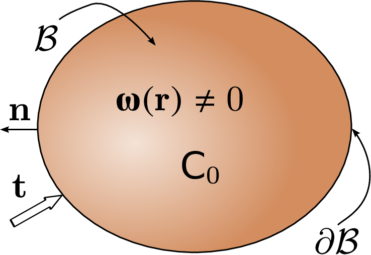
If an external traction force $\mathbf{t(r)}$ is applied to the boundary ${\partial\mathcal{B}}$ of $\mathcal{B}$, the resulting strain field $\mathbf{u}$ is a solution of the boundary value problem,

$$\begin{cases}\left(\sigma_{ij}+\omega_{ij}\right)_{,j}=0,\\ \sigma_{ij}n_{j}\Big|_{\partial\mathcal{B}}=t_{i},\end{cases}$$

(40)

supplemented by the constitutive relation (Hooke’s law):

$$\bm{\upsigma}=\mathsf{C}_{0}\bm{\upvarepsilon}.$$

(41)

Equation (40) is Newton’s 3rd law, the top and the bottom entry corresponding to the bulk and surface response respectively. The unit vector $\mathbf{n}$ is an external normal to ${\partial\mathcal{B}}$. The quantities $\bm{\upsigma}$ and $\bm{\upvarepsilon}$ are, respectively, the elastic stress and strain inside $\mathcal{B}$. The strain $\bm{\upvarepsilon}$ is defined in Eq. (1).

Since individual minima respond purely elastically, the strain field $\varepsilon_{ij}$ is compatible, ${\operatorname{inc}\,}\bm{\upvarepsilon}=0$, cf. Eq. (4). In contrast, the strain $\bm{\upeta}({\mathbf{r}})$ that corresponds to the internal stress $\bm{\upomega}({\mathbf{r}})$, $\bm{\upomega}=\mathsf{C}_{0}\bm{\upeta}$, can not be represented as a derivative of a single-valued deformation field. The field $\bm{\upeta}$ is thus incompatible:

$$\left({\operatorname{inc}\,}\bm{\upeta}\right)_{ij}=-\epsilon_{ikl}\epsilon_{jmn}\eta_{ln,km}\neq 0.$$

(42)

Both ${\mathbf{t}}({\mathbf{r}})$ and $\bm{\upomega}$ cause deformation in $\mathcal{B}$, as already mentioned. Consequently, the elastic stress $\bm{\upsigma}$ is a sum of two components:

$$\bm{\upsigma}=\bm{\upsigma}^{\text{{t}}}+\bm{\upsigma}^{\text{{s}}},$$

(43)

where the stress $\bm{\upsigma}^{\text{{t}}}$, produced by the surface traction, obeys

$$\begin{cases}\sigma^{\text{{t}}}_{ij,j}=0,\\ \sigma^{\text{{t}}}_{ij}n_{j}\Big|_{\partial\mathcal{B}}=t_{i},\end{cases}$$

(44)

while the stress $\bm{\upsigma}^{\text{{s}}}$, produced by the source field $\bm{\upomega}$, satisfies

$$\begin{cases}\left(\sigma^{\text{{s}}}_{ij}+\omega_{ij}\right)_{,j}=0,\\ \sigma^{\text{{s}}}_{ij}n_{j}\Big|_{\partial\mathcal{B}}=0.\end{cases}$$

(45)

The equation above follows from Eqs. (40) and (44). The elastic strain $\bm{\upvarepsilon}$ can be similarly written as a sum of two components,

$$\bm{\upvarepsilon}=\bm{\upvarepsilon}^{\text{{t}}}+\bm{\upvarepsilon}^{\text{{s}}},$$

(46)

where the strain produced by the traction force $\mathbf{t}$ and the internal stress $\bm{\upomega}$ are defined as

$$\bm{\upsigma}^{\text{{t}}}=\mathsf{C}_{0}\bm{\upvarepsilon}^{\text{{t}}}\text{\qquad{and}\qquad}\bm{\upsigma}^{\text{{s}}}=\mathsf{C}_{0}\bm{\upvarepsilon}^{\text{{s}}}$$

(47)

respectively. No built-in sources of stress lie at the boundary ${\partial\mathcal{B}}$ of the sample,

$$\bm{\upomega}\Big|_{\partial\mathcal{B}}=0,$$

(48)

and the present analysis is limited to symmetric sources

$$\omega_{ij}=\omega_{ji}.$$

(49)

The above boundary conditions for $\bm{\upomega}$ are standard in treatments of defects in solids.[68] These conditions entail an important relation between the volume averages of $\bm{\upsigma}^{\text{{s}}}$ and $\bm{\upomega}$,

$$\overline{\bm{\upsigma}^{\text{{s}}}}=\mathsf{C}_{0}\overline{\bm{\upvarepsilon}^{\text{{s}}}}=-\overline{\bm{\upomega}},$$

(50)

which is straightforward to show by writing $\sigma^{\text{{s}}}_{ij}=\sigma^{\text{{s}}}_{ik}x_{k,j}$ and using Gauss’s theorem together with Eq. (45).[69] Hereafter we use bars to indicate averaging over the volume $V$ of $\mathcal{B}$. For instance,

$$\overline{\bm{\upomega}}=\frac{1}{V}\int_{\mathcal{B}}\bm{\upomega}\;{\mathrm{d}V}.$$

(51)

Since our liquid is equilibrated, ensemble averaging is equivalent to time averaging.

By Eq. (50), the built-in stress pattern $\overline{\bm{\upomega}}$ automatically reflects the symmetry of $\mathsf{C}_{0}$ in the limiting cases of a uniform liquid, $\mu_{0}=0$, and of an infinitely compressible body, $\kappa_{0}=0$. Indeed, $\mu_{0}=0\Rightarrow\mathsf{C}_{0}\propto\mathsf{J}$, and so Eq. (33) implies that for any $\overline{\bm{\upvarepsilon}^{\text{{s}}}}$, the internal stress $\overline{\bm{\upomega}}$ is purely hydrostatic. Likewise, in the other extreme $\kappa_{0}=0\Rightarrow\mathsf{C}_{0}\propto\mathsf{K}$, the tensor $\overline{\bm{\upomega}}$ is purely deviatoric.

Next, we determine the linear response of body $\mathcal{B}$ to an external load. We define the effective elastic moduli $\mathsf{C}$ of $\mathcal{B}$ as a fourth-rank tensor connecting the volume average of the total stress in $\mathcal{B}$ with the volume average of the total elastic strain:

$$\int_{\mathcal{B}}\left(\bm{\upsigma}+\bm{\upomega}\right){\mathrm{d}V}=\int_{\mathcal{B}}\left(\mathsf{C}_{0}\bm{\upvarepsilon}+\bm{\upomega}\right){\mathrm{d}V}\equiv\mathsf{C}\;\int_{\mathcal{B}}\bm{\upvarepsilon}\;{\mathrm{d}V}.$$

(52)

Note that by definition, $\mathsf{C}$ is spatially uniform and Eq. (52) is the elastic analog of Eq. (7). Definition (52) is equivalent to the relation

$$\int_{\mathcal{B}}\bm{\upsigma}^{\text{{t}}}{\mathrm{d}V}=\mathsf{C}\;\int_{\mathcal{B}}\bm{\upvarepsilon}\;{\mathrm{d}V},$$

(53)

which is easy to show using Eqs. (43) and (50). The equation above relates quantities directly accessible in experiment: the average total load $\overline{\bm{\upsigma}^{\text{{t}}}}$ applied to $\mathcal{B}$ and the average resulted deformation $\overline{\bm{\upvarepsilon}}$ of $\mathcal{B}$. Using Eq. (46), we can further rewrite Eq. (53) as

$$\mathsf{C}_{0}\overline{\bm{\upvarepsilon}^{\text{{t}}}}=\mathsf{C}(\overline{\bm{\upvarepsilon}^{\text{{t}}}}+\overline{\bm{\upvarepsilon}^{\text{{s}}}}).$$

(54)

In full correspondence with the above discussion of the symmetry of the built-in stress $\overline{\bm{\upomega}}$, $\mathsf{C}\propto\mathsf{J}$ for a uniform liquid, $\mu_{0}=0$, while $\mathsf{C}\propto\mathsf{K}$ for an infinitely compressible solid, $\kappa_{0}=0$. We note that both cases correspond to fixed points on the $\nu_{0}\mapsto\nu$ mapping, where $\nu_{0}$ and $\nu$ are the bare and effective values of the Poisson ratio. Indeed, by Eq. (35), two isotropic fourth-rank tensors can be proportional to each other only if their Poisson ratios are equal. This notion will resurface in Section VII.

Since $\mathsf{C}$ should not depend on the configuration of the load and the shape of $\mathcal{B}$, we may conveniently assume a homogeneous $\bm{\upvarepsilon}^{\text{{t}}}$. Under these circumstances, the 2nd equality in Eq. (52) yields:

$$\mathsf{C}\overline{\bm{\upvarepsilon}}=\mathsf{C}_{0}\overline{\bm{\upvarepsilon}}+\overline{\bm{\upomega}}.$$

(55)

c.f. Eq. (7).

Thus, $\overline{\bm{\upomega}}$ is a function of the average strain $\overline{\bm{\upvarepsilon}}$ in the material. Analogously to Eq. (8), one has in the linear-response regime:

$$\overline{\omega}_{ij}=\mathsfit{X}^{\text{{s}}}_{ijkl}\overline{\varepsilon}_{kl},$$

(56)

where we define the static susceptibility $\mathsfit{X}^{\text{{s}}}_{ijkl}$ according to:

$$\mathsfit{X}^{\text{{s}}}_{ijkl}\equiv\frac{\partial\overline{\omega}_{lm}}{\partial\overline{\varepsilon}_{kl}}\Bigg|_{\overline{\bm{\upvarepsilon}}=0},$$

(57)

c.f. Eq. (9). This results, together with Eq. (55), in a linear response-type relation between the effective and “bare” elastic moduli of $\mathcal{B}$:

$$\mathsf{C}=\mathsf{C}_{0}+\mathsf{X}^{\text{{s}}}.$$

(58)

Here we have used that $\overline{\bm{\upomega}}=0$ in the absence of external load. Equation (58) is the elastic analog of Eq. (10). It is valid for any symmetry of the tensor $\mathsf{C}_{0}$. The following analysis is limited to isotropic elasticity, which is the simplest, yet most relevant case for amorphous materials. The “bare” elastic moduli, comprising the tensor $\mathsf{C}_{0}$, will be labelled $\mu_{0}$, $\kappa_{0}$, and $\nu_{0}$; these are the shear and bulk modulus, and the Poisson ratio, respectively. We expect $\mathsf{C}$ to be isotropic as well, since, by definition, amorphous materials are isotropic in the long-wavelength limit. Therefore, the susceptibility $\mathsf{X}^{\text{{s}}}$ must be an isotropic tensor to satisfy Eq. (58). Consequently, the tensor equation (58) is equivalent to two scalar equations, as discussed Section III. The effective moduli comprising $\mathsf{C}$ will be labelled $\mu$, $\kappa$, and $\nu$. By Eq. (58) they can be determined with the knowledge of the response function (57).

As in the dielectric case, calculation of the susceptibility (57) requires a specific microscopic model for the dynamics of $\bm{\upomega}$. Here we explicitly obtain such a microscopic model, which is the elastic analog of the dipole-dipole interaction in electrostatics.

In an earlier publication,[29] which will be referred to as BL, we have put forth a minimal ansatz for the stress distribution in equilibrated amorphous systems,[29] as explained in the Introduction, see Eq. (2). BL have shown that the dependence of the free energy $F$ on the magnitude of built-in stress $g$ is concave at small and large values of $g$, but has a convex portion at intermediate values of $g$. The low and high-$g$ states can thus be interpreted as distinct phases separated by a nucleation barrier. The high $g$ phase is aperiodic and vastly degenerate, the degeneracy originating from the multitude of mutual configurations of the degree of freedom $\bm{\upeta}$, which has 5 independent components, in view of the constraint (3). Given sufficient steric stabilization for aperiodic structures, the high $g$ phase can be made metastable implying the built-in stress can be self-consistently finite.

The interaction between the anharmonic degrees of freedom $\bm{\upeta}$ is determined by integrating out the long-wavelength motions:[29]

$$\mathcal{H}_{0}=\mathcal{H}_{\text{SE}}+a^{6}\sum_{m<n}\bm{\upeta}({\mathbf{r}}_{n})\mathsf{C}_{0}\mathsf{G}({\mathbf{r}}_{m}-{\mathbf{r}}_{n})\mathsf{C}_{0}\bm{\upeta}({\mathbf{r}}_{n}),$$

(59)

where the double sums are over all bead pairs. The quantity $\mathcal{H}_{\text{SE}}$ is the self-energy of the built-in stress in the absence of external load, see below. The coupling $\mathsf{G}$ is the Fourier transform,

$$\mathsf{G}({\mathbf{r}})=-\int_{|{\mathbf{k}}|\leq\frac{\pi}{a}}\frac{d^{3}({\mathbf{k}})}{(2\pi)^{3}}\cos({\mathbf{k}}{\mathbf{r}})\;\widetilde{\mathsf{G}}({\mathbf{k}}),$$

(60)

of the following tensor:

$$\widetilde{\!\mathsfit{G}}_{ijml}=\frac{1}{\mu_{0}}\left(\delta_{im}\hat{k}_{j}\hat{k}_{l}+\delta_{il}\hat{k}_{j}\hat{k}_{m}+\delta_{jm}\hat{k}_{i}\hat{k}_{l}+\delta_{jl}\hat{k}_{i}\hat{k}_{m}-\frac{\lambda_{0}+\mu_{0}}{\lambda_{0}+2\mu_{0}}\hat{k}_{i}\hat{k}_{j}\hat{k}_{m}\hat{k}_{l}\right),$$

(61)

where $\hat{{\mathbf{k}}}\equiv{\mathbf{k}}/|{\mathbf{k}}|$. Recasting Eq. (59) in terms of the internal stress $\bm{\upomega}=\mathsf{C}_{0}\bm{\upeta}$ we obtain

$$\mathcal{H}_{0}=\frac{1}{2}\int_{\mathcal{B}}{\mathrm{d}V}\bm{\upomega}\mathsf{C}_{0}^{-1}\bm{\upomega}+\frac{1}{2}\int_{\mathcal{B}}{\mathrm{d}V}\int_{\mathcal{B}}{\mathrm{d}V}^{\prime}\omega_{ij}({\mathbf{r}})\,\mathsfit{G}_{ijlm}(\mathbf{r}-\mathbf{r}^{\prime})\,\omega_{lm}(\mathbf{r}^{\prime}),$$

(62)

where we assume the built-in stress $\bm{\upomega}$ and deformation $\bm{\upeta}$ are related by Hooke’s law: $\bm{\upomega}=\mathsf{C}_{0}\bm{\upeta}$. Switching from discrete summation over bead sites to spatial integration is done according to the prescription $a^{3}\sum\to\int{\mathrm{d}V}$. The first integral on the r.h.s. of Eq. (62) corresponds to the self-energy from Eq. (59).

The expression for the coupling $\mathsf{G}$ between local sources of stress $\bm{\upomega}$, Eq. (60), can be written out explicitly as:

$$\begin{split}\mathsfit{G}_{ijml}(\mathbf{r}-\mathbf{r}^{\prime})&=\frac{1}{64\pi^{3}\mu_{0}\left(1-\nu_{0}\right)}\left(\delta_{ip}\frac{\partial}{\partial x_{j}}+\delta_{jp}\frac{\partial}{\partial x_{i}}\right)\left(\delta_{ql}\frac{\partial}{\partial x_{m}}+\delta_{qm}\frac{\partial}{\partial x_{l}}\right)\\ &\times\left(2\left(1-\nu_{0}\right)\delta_{pq}\frac{\partial^{2}}{\partial x_{s}x_{s}}-\frac{\partial^{2}}{\partial x_{p}x_{q}}\right)\int_{\lvert{\mathbf{k}}\rvert\leq\frac{\pi}{a}}\mathrm{d}\mathbf{k}\frac{e^{i\mathbf{k}(\mathbf{r}-\mathbf{r}^{\prime})}}{k^{4}}.\end{split}$$

(63)

In the long-wavelength limit, $(r\rightarrow\infty)\Rightarrow(a\rightarrow 0)$, the above expression simplifies significantly as the integral reduces to $\int\mathrm{d}\mathbf{k}\exp\!\left[i\mathbf{k}\mathbf{r}\right]/k^{4}=-\pi^{2}r$.[39] The stress-stress coupling, which we label in this approximation by $\mathsf{G}^{\text{{a}}}$, can be now expressed via the well known Green tensor ${\bm{\upgamma}^{\text{{a}}}}$ for a point force inside an infinite, homogeneous, and isotropic medium (Kelvin’s solution)[39] with the elastic moduli tensor $\mathsf{C}_{0}$:

$$\mathsfit{G}^{\text{{a}}}_{ijml}(\mathbf{r}-\mathbf{r}^{\prime})=\frac{1}{4}\left(\delta_{ip}\frac{\partial}{\partial x_{j}}+\delta_{jp}\frac{\partial}{\partial x_{i}}\right)\left(\delta_{ql}\frac{\partial}{\partial x_{m}}+\delta_{qm}\frac{\partial}{\partial x_{l}}\right){\gamma}^{\text{{a}}}_{pq}(\mathbf{r}-\mathbf{r}^{\prime}),$$

(64)

where

$${\gamma}^{\text{{a}}}_{ij}({\mathbf{r}})=\dfrac{1}{16\pi\mu_{0}\left(1-\nu_{0}\right)}\dfrac{1}{r}\left[\left(3-4\nu_{0}\right)\delta_{ij}+\dfrac{x_{i}x_{j}}{r^{2}}\right].$$

(65)

Note that, apart from the complicated tensorial form of the coupling, the (long-wavelength) distance dependence of $\mathsf{G}^{\text{{a}}}$ is $\propto 1/r^{3}$, analogously to the electric dipole-dipole interaction. The tensor ${\bm{\upgamma}^{\text{{a}}}}({\mathbf{r}})$ describes the response of the elastic medium to point-force localized at the origin. Note that this response diverges for a uniform liquid, $\mu_{0}=0$. This is expected since even an infinitesimal force causes an infinite displacement in a uniform liquid, and so linear elasticity is no longer applicable. Note that in the opposite extreme of an infinitely compressible body, $\kappa_{0}=0$ or $\nu_{0}=-1$, the kernel ${\bm{\upgamma}^{\text{{a}}}}$ is well defined. As shown in Appendix A, $\mathsf{G}^{\text{{a}}}({\mathbf{r}})$ is the tensor describing the elastic response to a point-source of stress by an infinite, homogeneous, and isotropic medium. The elastic strain $\bm{\upvarepsilon}^{\text{{s}}}$ produced by $\bm{\upomega}$ can thus be written as

$$\bm{\upvarepsilon}^{\text{{s}}}({\mathbf{r}})=\int_{\mathcal{B}}{\mathrm{d}V}^{\prime}\mathsf{G}^{\text{{a}}}(\mathbf{r}-\mathbf{r}^{\prime})\bm{\upomega}(\mathbf{r}^{\prime}),$$

(66)

so that the Hamiltonian (62) becomes

$$\mathcal{H}_{0}\approx\mathcal{H}^{\text{{a}}}_{0}=\frac{1}{2}\int_{\mathcal{B}}{\mathrm{d}V}\bm{\upomega}\left(\bm{\upvarepsilon}^{\text{{s}}}+\mathsf{C}_{0}^{-1}\bm{\upomega}\right),$$

(67)

where the superscript “A” indicates that the long-wavelength limit of the Green’s function is used.

In the presence of an external traction force, $\bm{\upvarepsilon}^{\text{{t}}}\neq 0$, $\mathcal{H}_{0}$ must be supplemented by an appropriate coupling term. We will show systematically in Section VI, see Eq. (90), that this coupling is equal to the expected $\int_{\mathcal{B}}{\mathrm{d}V}\bm{\upvarepsilon}^{\text{{t}}}\bm{\upomega}$. Hence, the full Hamiltonian for the internal stress in the presence of the external load reads

$$\mathcal{H}^{\text{{a}}}=\mathcal{H}^{\text{{a}}}_{0}+\int_{\mathcal{B}}{\mathrm{d}V}\bm{\upvarepsilon}^{\text{{t}}}\bm{\upomega}.$$

(68)

The linear response of the system to externally imposed deformation field $\bm{\upvarepsilon}^{\text{{t}}}({\mathbf{r}})$ is described, in the standard fashion, by the second order isothermal response function

	$\displaystyle\mathsfit{X}_{ijkl}({\mathbf{r}},{\mathbf{r}}^{\prime})$	$\displaystyle=$	$\displaystyle\frac{\delta\langle\omega_{ij}({\mathbf{r}})\rangle}{\delta\varepsilon^{\text{{t}}}_{kl}({\mathbf{r}}^{\prime})}\Bigg|_{\bm{\upvarepsilon}^{\text{{t}}}=0}=\frac{\delta}{\delta\varepsilon^{\text{{t}}}_{kl}({\mathbf{r}}^{\prime})}\frac{\int\mathcal{D}\bm{\upomega}\,\omega_{ij}({\mathbf{r}})\exp\left[-\beta\mathcal{H}^{\text{{a}}}\right]}{\int\mathcal{D}\bm{\upomega}\exp\left[-\beta\mathcal{H}^{\text{{a}}}\right]}\Bigg|_{\bm{\upvarepsilon}^{\text{{t}}}=0}$		(69)
		$\displaystyle=$	$\displaystyle-\beta\Big[\langle\omega_{ij}({\mathbf{r}})\omega_{kl}({\mathbf{r}}^{\prime})\rangle_{0}-\langle\omega_{ij}({\mathbf{r}})\rangle_{0}\langle\omega_{kl}({\mathbf{r}}^{\prime})\rangle_{0}\Big],$

where the naught on the r.h.s. indicates averaging in zero field, $\bm{\upvarepsilon}^{\text{{t}}}=0$, by $\langle\cdots\rangle_{0}$. For instance,

$$\langle\bm{\upomega}({\mathbf{r}})\rangle_{0}=\frac{\int\mathcal{D}\bm{\upomega}\,\bm{\upomega}({\mathbf{r}})\,\exp\!\left[-\beta\mathcal{H}_{0}^{\text{{a}}}\right]}{\int\mathcal{D}\bm{\upomega}\,\exp\!\left[-\beta\mathcal{H}_{0}^{\text{{a}}}\right]}.$$

(70)

By the chain rule of differentiation,

$$\langle\omega_{ij}({\mathbf{r}})\rangle=\int{\mathrm{d}V}^{\prime}\frac{\delta\langle\omega_{ij}({\mathbf{r}})\rangle}{\delta\varepsilon^{\text{{t}}}_{kl}({\mathbf{r}}^{\prime})}\Bigg|_{\bm{\upvarepsilon}^{\text{{t}}}=0}\varepsilon^{\text{{t}}}_{kl}({\mathbf{r}}^{\prime}),$$

(71)

and so the standard sum rule for the static isothermal susceptibility $\widetilde{\mathsf{X}}^{\text{{s}}}$ holds:

$$\langle\omega_{ij}\rangle=\varepsilon^{\text{{t}}}_{kl}\int{\mathrm{d}V}^{\prime}\mathsfit{X}_{ijkl}({\mathbf{r}},{\mathbf{r}}^{\prime})=\widetilde{\!\mathsfit{X}}^{\text{{s}}}_{ijkl}\varepsilon^{\text{{t}}}_{kl}.$$

(72)

We use the tilde to distinguish $\widetilde{\mathsf{X}}^{\text{{s}}}$ from the susceptibility defined by Eq. (57) because it corresponds to the derivative of $\langle{\bm{\upomega}}\rangle$ with respect to the average field $\overline{\bm{\upvarepsilon}}$, whereas $\widetilde{\mathsf{X}}^{\text{{s}}}$ is equal to the derivative with respect to $\bm{\upvarepsilon}^{\text{{t}}}$. The two fields are straightforwardly related by Eq. (54).

Evaluation of the cumulant in Eq. (69) is prohibitively difficult to accomplish analytically for the model in Eq. (62). However, because of the Coulomb-like distance dependence of the interaction between point sources of force, we may proceed by analogy with the electric dipole-dipole interaction, for which Onsager’s cavity method can be employed. The analogy between elasticity of stressed continua and electrostatics of polar dielectrics was noticed a long time ago and used primarily to study crystalline materials with a low concentration of defects.[60, 70] Periodic lattices are anisotropic, which usually implies there at most few, discrete states of an individual defect.[71] The same thing can be said about orientational glasses, which are periodic crystals containing anisotropic substitutional impurities, whose orientations are random given sufficiently high density and/or low temperature.[72] Reorientational dynamics of such impurities lead to a marked temperature dependence of the elastic moduli.[73, 72]

We have shown earlier,[29] see also Sec. VII below, that constraint (3) is equivalent to fixing the length of a certain $6$-component vector. Thus the structural dynamics of the built-in stress correspond to the rotations of interacting $6$-vectors. This makes an effective field approximation for the elasticity of supercooled liquids conceptually very similar to that for the dielectric properties of polar liquids. In fact, as we will show below, it is possible to generalize Onsager’s cavity construction to find a relation between the bare and renormalized elastic moduli of a supercooled liquid. This relation is controlled by the magnitude of the built-in stress, similarly to how the bare and renormalized dielectric constants are related via the magnitude of the molecular dipole in Eq. (18).

Consider an ellipsoidal region $\mathcal{I}$ inside the body $\mathcal{B}$. We will treat this region explicitly, whereby the region is characterized by bare elastic constants $\mathsf{C}_{0}$ and an intrinsic distribution of built-in stress $\bm{\upomega}$. In contrast, the built-in stress outside the region will be treated effectively; we will approximate the response of the environment as an elastic continuum with effective elastic constants $\mathsf{C}$, see Fig. 2. Our aim is to determine these effective elastic constants $\mathsf{C}$ self-consistently. We emphasize that this approach is not merely phenomenological, while being surely consonant with observation. Its validity has the same origin as the theory of dielectrics and stems from the fact that the electric field due to an infinite, uniformly charged plane is coordinate independent (within the individual half-spaces), leading to a uniform polarization-induced field inside a polarizable slab subject to a uniform external field. In turn, this notion stems from the $1/r$ dependence of the Green’s function for electrostatic and elastic interactions, which has to do with the lack of mass for photons and phonons respectively.

Since both $\mathsf{C}_{0}$ and $\mathsf{C}$ are assumed to be isotropic, all possible orientations of $\mathcal{I}$ in $\mathcal{B}$ are equivalent. The linear size of $\mathcal{B}$, $L_{\mathcal{B}}$, is assumed to be much larger than that of $\mathcal{I}$; consequently, we neglect the image forces produced by ${\partial\mathcal{B}}$ since the corresponding contribution is $\propto L_{\mathcal{B}}^{-3}$. A key feature of the construction is that it neglects correlations between the sources of built-in stress inside and outside of $\mathcal{I}$ for the purpose of estimating $\langle\bm{\upomega}\rangle$. This is a good approximation, if the size of $\mathcal{I}$ is larger than the correlation length of the stress distribution $\bm{\upomega}$. The thermodynamic average $\langle\bm{\upomega}\rangle$ is then approximated by Boltzmann averaging over all structural states inside $\mathcal{I}$ only.

First off, the full elastic energy of $\mathcal{B}$ that contains an inclusion $\mathcal{I}$ containing sources of built-in stress $\bm{\upomega}$ is equal to

$$\mathcal{E}_{el}=\frac{1}{2}\int_{\mathcal{B}}{\mathrm{d}V}\left(\bm{\upsigma}+\bm{\upomega}\right)\left(\bm{\upvarepsilon}+\mathsf{C}_{0}^{-1}\bm{\upomega}\right),$$

(73)

where the integrand is the product of the total (compatible and incompatible) stress, $\bm{\upsigma}+\bm{\upomega}$, and the total strain, $\bm{\upvarepsilon}+\mathsf{C}_{0}^{-1}\bm{\upomega}$. The elastic stress $\bm{\upsigma}$ and strain $\bm{\upvarepsilon}$ are solutions of Eq. (40), but since $\mathcal{B}$ now contains an inhomogeneity in the form of the elastic discontinuity at the region boundary $\partial\mathcal{I}$, Eq. (43) no longer holds. The total elastic stress now has to include a contribution from the stress “polarization” at the region boundary:

$$\bm{\upsigma}=\bm{\upsigma}^{\text{{t}}}+\bm{\upsigma}^{\text{{p}}}+\bm{\upsigma}^{\text{{s}}},$$

(74)

where

$$\bm{\upsigma}^{\text{{t}}}=\mathsf{C}\,\bm{\upvarepsilon}^{\text{{t}}}$$

(75)

everywhere in $\mathcal{B}$; $\bm{\upsigma}^{\text{{t}}}$ satisfies (44). The quantity

$$\bm{\upsigma}^{\text{{p}}}=\begin{cases}\mathsf{C}\bm{\upvarepsilon}^{\text{{p}}},\text{ outside }\mathcal{I},\\ \mathsf{C}_{0}\bm{\upvarepsilon}^{\text{{p}}},\text{ inside }\mathcal{I},\end{cases}$$

(76)

is the stress produced by the boundary $\partial\mathcal{I}$, while $\bm{\upsigma}^{\text{{s}}}$ is the stress produced by $\bm{\upomega}$. As before, $\bm{\upsigma}^{\text{{s}}}$ is given by the solution of (45) but the constitutive relations are now different between the region and the environment:

$$\bm{\upsigma}^{\text{{s}}}=\begin{cases}\mathsf{C}\bm{\upvarepsilon}^{\text{{s}}},\text{ outside }\mathcal{I},\\ \mathsf{C}_{0}\bm{\upvarepsilon}^{\text{{s}}},\text{ inside }\mathcal{I}.\end{cases}$$

(77)

Analogously to $\bm{\upsigma}^{\text{{s}}}$, the stress $\bm{\upsigma}^{\text{{p}}}$ must satisfy the free traction boundary conditions on the surface of $\mathcal{B}$:

$$\sigma^{\text{{p}}}_{ij}n_{j}\Big|_{\partial\mathcal{B}}=0.$$

(78)

Next we use the cavity construction to evaluate the response function (57). First we need to establish a correspondence between the homogeneous set-up of Section IV and the present situation with an elastic discontinuity at the region boundary $\partial\mathcal{I}$. The traction forces in both cases are equal to each other analogously to how the dielectric displacement is not modified, on average, by introducing a cavity. Further, by Eqs. (75) and (53), we establish that the traction displacement $\bm{\upvarepsilon}^{\text{{t}}}$ outside the inclusion $\mathcal{I}$ corresponds with the average strain $\overline{\bm{\upvarepsilon}}$ defined in Section IV. Thus, the static susceptibility $\mathsf{X}^{\text{{s}}}$ from Eq. (57) must be evaluated via

$$\mathsfit{X}^{\text{{s}}}_{ijkl}=\frac{\partial\overline{\omega}_{ij}}{\partial\varepsilon^{\text{{t}}}_{kl}}\Bigg|_{\bm{\upvarepsilon}^{\text{{t}}}=0}.$$

(79)

From here on, we assume $\bm{\upsigma}^{\text{{t}}}$ and $\bm{\upvarepsilon}^{\text{{t}}}$ are homogeneous. Then, for an ellipsoidal region $\mathcal{I}$, $\bm{\upvarepsilon}^{\text{{p}}}$ inside $\mathcal{I}$ is also homogeneous and is given by[74, 61, 69]

$$\bm{\upvarepsilon}^{\text{{p}}}=\mathsf{S}\mathsf{Q}\left(\mathsf{C}-\mathsf{C}_{0}\right)\bm{\upvarepsilon}^{\text{{t}}},$$

(80)

where

$$\mathsf{Q}\equiv\left(\mathsf{C}-\left[\mathsf{C}-\mathsf{C}_{0}\right]\mathsf{S}\right)^{-1},$$

(81)

and $\mathsf{S}$ is the so-called Eshelby tensor.[61] The Eshelby tensor appears in continuum mechanics as the solution to the following problem: Imagine that a region $\mathcal{I}$ inside a homogeneous elastic continuum with moduli $\mathsf{C}$ experiences a structural transformation, such as a martensitic transition. Under these circumstances the region would relax to attain a uniform stress-free strain $\bm{\upvarepsilon}^{\ast}$, if removed from the matrix. What is the deformation $\tilde{\bm{\upvarepsilon}}$ of the region $\mathcal{I}$, if it remains inside the matrix? Eshelby has shown that[75]

$$\tilde{\bm{\upvarepsilon}}=\mathsf{S}\,\bm{\upvarepsilon}^{\ast},$$

(82)

where the tensor $\mathsf{S}$ is generally a function of the coordinate and depends on the shape of the region $\mathcal{I}$. If $\mathcal{I}$ is an ellipsoid, however, the Eshelby tensor is spatially uniform, and so is $\tilde{\bm{\upvarepsilon}}$. Despite its uniformity (for ellipsoidal $\mathcal{I}$), $\mathsf{S}$ is generally not isotropic, and so the order of multiplication in Eq. (80) matters. If, however, $\mathcal{I}$ is spherical, $\mathsf{S}$ does become isotropic:

$$\mathsf{S}=\frac{1}{3\left(1-\nu\right)}\;\mathsf{L}\!\left[{1+\nu}\,,\,{\frac{2}{5}\left(4-5\nu\right)}\right].$$

(83)

The last equation applies also when the elastic moduli experience a discontinuity at the region boundary, the case we are interested here. Note that $\mathsf{S}$ depends only on the Poisson ratio of the matrix, i.e. the part of $\mathcal{B}$ outside $\mathcal{I}$. Also, for $\nu=1/5$, the Eshelby tensor is proportional to the unit tensor $\mathsf{I}$,

$$\mathsf{S}\Big|_{\nu=1/5}=\frac{1}{2}\mathsf{I},$$

(84)

so that $\tilde{\bm{\upvarepsilon}}=\bm{\upvarepsilon}^{\ast}/2$, i.e., $\tilde{\bm{\upvarepsilon}}$ and $\bm{\upvarepsilon}^{\ast}$ are related via a scalar. This is a peculiar situation, in which the self-consistent tensor equation (58) boils down to a single scalar equation, as we shall see in Sec. VII. Hereby the bulk and shear modulus are renormalized in equal measure so that $\nu$ remains equal to $\nu_{0}=1/5$.

References

- [1] V. Lubchenko and P. G. Wolynes, J. Chem. Phys. 119, 9088 (2003a).
- [2] V. Lubchenko and P. G. Wolynes, “Theories of Structural Glass Dynamics: Mosaics, Jamming, and All That,” in Structural Glasses and Supercooled Liquids: Theory, Experiment, and Applications, edited by P. G. Wolynes and V. Lubchenko (John Wiley & Sons, 2012) pp. 341–379.
- [3] F. Mezei and M. Russina, J. Phys. Cond. Mat. 11, A341 (1999).
- [4] Y. Singh, J. P. Stoessel, and P. G. Wolynes, Phys. Rev. Lett. 54, 1059 (1985).
- [5] P. Rabochiy and V. Lubchenko, J. Phys. Chem. B 116, 5729 (2012a).
- [6] T. R. Kirkpatrick, D. Thirumalai, and P. G. Wolynes, Phys. Rev. A 40, 1045 (1989).
- [7] X. Xia and P. G. Wolynes, Proc. Natl. Acad. Sci. 97, 2990 (2000).
- [8] V. Lubchenko and P. G. Wolynes, Annu. Rev. Phys. Chem. 58, 235 (2007a).
- [9] V. Lubchenko and P. G. Wolynes, Phys. Rev. Lett. 87, 195901 (2001).
- [10] S. Ashtekar, G. Scott, J. Lyding, and M. Gruebele, J. Phys. Chem. Lett. 1, 1941 (2010).
- [11] U. Tracht, M. Wilhelm, A. Heuer, H. Feng, K. Schmidt-Rohr, and H. W. Spiess, Phys. Rev. Lett. 81, 2727 (1998).
- [12] E. V. Russell and N. E. Israeloff, Nature 408, 695 (2000).
- [13] M. T. Cicerone and M. D. Ediger, J. Chem. Phys. 104, 7210 (1996).
- [14] S. Capaccioli, G. Ruocco, and F. Zamponi, J. Phys. Chem. B 112, 10652 (2008).
- [15] P. Rabochiy, P. G. Wolynes, and V. Lubchenko, J. Phys. Chem. B 117, 15204 (2013).
- [16] V. Lubchenko, Proc. Natl. Acad. Sci. 106, 11506 (2009).
- [17] L. Onsager, J. Am. Chem. Soc. 58, 1486 (1936).
- [18] P. Debye, Physik. Z. 13, 97 (1912).
- [19] P. Debye, Polar molecules (Dover, 1945).
- [20] J. G. Kirkwood, J. Chem. Phys. 7, 911 (1939).
- [21] S. Alexander, Phys. Rep. 296, 65 (1998).
- [22] M. Bienfait, Surf. Sci. 272, 1 (1972).
- [23] H. Taub, G. Torzo, H. J. Lauter, and S. C. Fain Jr., eds., Phase Transitions in Surface Films 2, NATO ASI Series B, Vol. 267 (Plenum Press, 1991).
- [24] S. Sachdev and D. R. Nelson, Phys. Rev. B 32, 1480 (1985).
- [25] Z. Nussinov, Phys. Rev. B 69, 014208 (2004).
- [26] T. Egami and D. Srolovitz, J. Phys. F: Met. Phys. 12, 2141 (1982).
- [27] D. Srolovitz, K. Maeda, V. Vitek, and T. Egami, Phil. Mag. A 44, 847 (1981).
- [28] H. Mizuno, S. Mossa, and J.-L. Barrat, Europhys. Lett. 104, 56001 (2013).
- [29] D. Bevzenko and V. Lubchenko, J. Phys. Chem. B 113, 16337 (2009).
- [30] L. D. Landau and E. M. Lifshitz, Theory of Elasticity (Pergamon Press, 1986).
- [31] L. Yan, G. Düring, and M. Wyart, Proc. Natl. Acad. Sci. 110, 6307 (2013).
- [32] H. Yoshino and M. Mézard, Phys. Rev. Lett. 105, 015504 (2010).
- [33] H. Yoshino, J. Chem. Phys. 136, 214108 (2012).
- [34] B. W. H. van Beest, G. J. Kramer, and R. A. van Santen, Phys. Rev. Lett. 64, 1955 (1990).
- [35] E. Flenner, H. Staley, and G. Szamel, Phys. Rev. Lett. 112, 097801 (2014).
- [36] G. Ayton, M. J. P. Gingras, and G. N. Patey, Phys. Rev. Lett. 75, 2360 (1995).
- [37] J. Tomasi and M. Persico, Chem. Rev. 94, 2027 (1994).
- [38] M. Baus and R. Lovett, Phys. Rev. A 44, 1211 (1991).
- [39] C. Teodosiu, Elastic Models of Crystal Defects (Springer, 1982).
- [40] E. Kröner, Int. J. Sol. Struct. 29, 1849 (1992).
- [41] V. Lubchenko and P. G. Wolynes, Adv. Chem. Phys. 136, 95 (2007b).
- [42] A. Zhugayevych and V. Lubchenko, J. Chem. Phys. 132, 044508 (2010a).
- [43] A. Zhugayevych and V. Lubchenko, J. Chem. Phys. 133, 234503 (2010b).
- [44] A. Zhugayevych and V. Lubchenko, J. Chem. Phys. 133, 234504 (2010c).
- [45] C. Cammarota and G. Biroli, Europhys. Lett. 98, 36005 (2012).
- [46] D. K. Biegelsen and R. A. Street, Phys. Rev. Lett. 44, 803 (1980).
- [47] M. A. Bösch and J. Shah, Phys. Rev. Lett. 42, 118 (1979).
- [48] S. Corezzi, S. Caponi, F. Rossi, and D. Fioretto, J. Phys. Chem. B 117, 14477 (2013).
- [49] F. Léonforte, A. Tanguy, J. P. Wittmer, and J.-L. Barrat, Phys. Rev. Lett. 97, 055501 (2006).
- [50] A. Paul, S. Sengupta, and M. Rao, J. Phys.: Condens. Matter 26, 015007 (2014).
- [51] H. Wagner, D. Bedorf, S. Küchemann, M. Schwabe, Z. Bo, W. Arnold, and K. Samwer, Nature Materials 10, 439 (2011).
- [52] S. G. Mayr, Phys. Rev. B 79, 060201 (2009).
- [53] W. Schirmacher, Europhys. Lett. 73, 892 (2006).
- [54] A. Marruzzo, W. Schirmacher, A. Fratalocchi, and G. Ruocco, Sci. Rep. 3, 1407 (2013).
- [55] E. Kröner, Arch. Ration. Mech. Anal. 4, 18 (1960).
- [56] P. Dederichs, C. Lehmann, H. Schober, A. Scholz, and R. Zeller, J. Nucl. Mat. 69-70, 176 (1978).
- [57] M. P. Puls, The Effect of Hydrogen and Hydrides on the Integrity of Zirconium Alloy Components: Delayed Hydride Cracking (Springer, 2012).
- [58] L. D. Landau and E. M. Lifshitz, Electrodynamics of Continuous Media (Pergamon Press, 1960).
- [59] J. D. Jackson, Classical Electrodynamics (Wiley, 1975).
- [60] E. Kröner, in Theory of Crystal Defects. Proc. of the Summer school held in Hrazany in September 1964 (Academic Press, 1966).
- [61] L. J. Walpole, Adv. App. Mech. 21, 169 (1981).
- [62] M. Mezard, G. Parisi, and M. Virasoro, Spin Glass Theory And Beyond (World Scientific, 1987).
- [63] T. R. Kirkpatrick and P. G. Wolynes, Phys. Rev. B 36, 8552 (1987a).
- [64] M. Mézard and G. Parisi, J. Chem. Phys. 111, 1076 (1999).
- [65] T. R. Kirkpatrick and P. G. Wolynes, Phys. Rev. A 35, 3072 (1987b).
- [66] J. Kurchan, G. Parisi, P. Urbani, and F. Zamponi, J. Phys. Chem. B 117, 12979 (2013).
- [67] P. G. Wolynes and V. Lubchenko, eds., Structural Glasses and Supercooled Liquids: Theory, Experiment, and Applications (John Wiley & Sons, 2012) pp. 341–379.
- [68] D. J. Bacon, D. M. Barnett, and R. O. Scattergood, Prog. Mater Sci. 23, 51 (1979).
- [69] T. Mura, Micromechanics of Defects in Solids (Martinus Nijhoff, 1987).
- [70] W. Känzig, J. Phys. Chem. Solids 23, 479 (1962).
- [71] A. Nowick and W. Heller, Adv. Phys. 12, 251 (1963).
- [72] A. Loidl, Annu. Rev. Phys. Chem. 40, 29 (1989).
- [73] R. M. Lynden-Bell and K. H. Michel, Rev. Mod. Phys. 66, 721 (1994).
- [74] J. D. Eshelby, Phil. Trans. Roy. Soc. A 244, 87 (1951).
- [75] J. D. Eshelby, Proc. Roy. Soc. A 241, 376 (1957).
- [76] H. L. Friedman, Molecular Physics 29, 1533 (1975).
- [77] M. M. Mehrabadi and S. C. Cowin, Q. J. Mech. Appl. Math. 43, 15 (1990).
- [78] J. P. Stoessel and P. G. Wolynes, J. Chem. Phys. 80, 4502 (1984).
- [79] M. Baus and J.-L. Colot, J. Phys. C: Solid State Phys. 19, L135 (1986).
- [80] H. Lowen, J. Phys.: Condens. Matter 2, 8477 (1990).
- [81] P. Rabochiy and V. Lubchenko, J. Chem. Phys. 136, 084504 (2012b).
- [82] S. M. Sharma and S. Sikka, Prog. Mater. Sci. 40, 1 (1996).
- [83] V. V. Brazhkin and A. G. Lyapin, J. Phys. Cond. Mat. 15, 6059 (2003).
- [84] E. Ponyatovsky and O. Barkalov, Mat. Sci. Rep. 8, 147 (1992).
- [85] R. J. Hemley, A. P. Jephcoat, H. K. Mao, L. C. Ming, and M. H. Manghnani, Nature 334, 52 (1988).
- [86] G. Parisi and F. Zamponi, Rev. Mod. Phys. 82, 789 (2010).
- [87] T. S. Grigera, V. Martin-Mayor, G. Parisi, and P. Verrocchio, Nature 422, 289 (2003).
- [88] A. C. Anderson, in Amorphous Solids: Low-Temperature Properties, edited by W. A. Phillips (Springer-Verlag, Berlin, Heidelberg, New York, 1981).
- [89] Y. P. Joshi, Phys. Stat. Sol. (b) 95, 317 (1979).
- [90] V. Lubchenko and P. G. Wolynes, Proc. Natl. Acad. Sci. 100, 1515 (2003b).
- [91] W. A. Phillips, ed., Amorphous Solids: Low-Temperature Properties (Springer-Verlag, Berlin, Heidelberg, New York, 1981).
- [92] J. Qu and M. Cherkaoui, Fundamentals of Micromechanics of Solids (John Wiley & Sons, Inc., 2006).
- [93] A. Abramowitz and I. Stegun, eds., Handbook of Mathematical Functions (Dover, 1964).
- [94] G. Mussardo, Statistical Field Theory: An Introduction to Exactly Solved Models in Statistical Physics (Oxford University Press, 2010).