跳到论文正文
W Papers独立论文阅读器 arXiv:1409.7193 论文正文 计算阅读时间 · 0%
引用这篇论文根据当前论文元数据生成,正式投稿前建议核对。


License: arXiv.org perpetual non-exclusive license
arXiv:1409.7193v2 [stat.ML] 19 Mar 2015

MIST: l0l_{0} Sparse Linear Regression with Momentum

Goran Marjanovic    Magnus O. Ulfarsson    †  Alfred O. Hero III ‡ ††thanks: Goran Marjanovic is with the School of Electrical Engineering and Telecommunications, University of New South Wales, Sydney, NSW, 2052 Australia (email: goran.m.marjanovic@gmail.com)††thanks: Alfred O. Hero III is with the Department of Electrical and Computer Science, University of Michigan, Ann Arbor, MI, 48109 USA (email: hero@eecs.umich.edu)††thanks: Magnus O. Ulfarsson is with the Department of Electrical Engineering, University of Iceland, Reykjavik, 107 Iceland (email: mou@hi.is)††thanks: † This work was partly supported by the Research Fund of the University of Iceland and the Icelandic Research Fund (130635-051).††thanks: ‡ This work was partially supported by ARO grant W911NF-11-1-0391.
Abstract

Significant attention has been given to minimizing a penalized least squares criterion for estimating sparse solutions to large linear systems of equations. The penalty is responsible for inducing sparsity and the natural choice is the so-called l0l_{0} norm. In this paper we develop a Momentumized Iterative Shrinkage Thresholding (MIST) algorithm for minimizing the resulting non-convex criterion and prove its convergence to a local minimizer. Simulations on large data sets show superior performance of the proposed method to other methods.

Index Terms: 
sparsity, non-convex, l0l_{0} regularization, linear regression, iterative shrinkage thresholding, hard-thresholding, momentum

I Introduction

In the current age of big data acquisition there has been an ever growing interest in sparse representations, which consists of representing, say, a noisy signal as a linear combination of very few components. This implies that the entire information in the signal can be approximately captured by a small number of components, which has huge benefits in analysis, processing and storage of high dimensional signals. As a result, sparse linear regression has been widely studied with many applications in signal and image processing, statistical inference and machine learning. Specific applications include compressed sensing, denoising, inpainting, deblurring, source separation, sparse image reconstruction, and signal classification, etc.

The linear regression model is given by:

𝐲=𝐀𝐱+ϵ,\displaystyle\mathbf{y}=\mathbf{A}\mathbf{x}+\bm{\epsilon}, (1)

where 𝐲d×1\mathbf{y}_{d\times 1} is a vector of noisy data observations, 𝐱m×1\mathbf{x}_{m\times 1} is the sparse representation (vector) of interest, 𝐀d×m\mathbf{A}_{d\times m} is the regression matrix and ϵd×1\bm{\epsilon}_{d\times 1} is the noise. The estimation aim is to choose the simplest model, i.e., the sparsest 𝐱\mathbf{x}, that adequately explains the data 𝐲\mathbf{y}. To estimate a sparse 𝐱\mathbf{x}, major attention has been given to minimizing a sparsity Penalized Least Squares (PLS) criterion [1, 2, 3, 4, 5, 6, 7, 8, 9, 10]. The least squares term promotes goodness-of-fit of the estimator while the penalty shrinks its coefficients to zero. Here we consider the non-convex l0l_{0} penalty since it is the natural sparsity promoting penalty and induces maximum sparsity. The resulting non-convex l0l_{0} PLS criterion is given by:

F⁡(𝐱)=12​‖𝐲−𝐀𝐱‖22+λ​‖𝐱‖0,\displaystyle F(\mathbf{x})=\frac{1}{2}\|\mathbf{y}-\mathbf{A}\mathbf{x}\|_{2}^{2}+\lambda\|\mathbf{x}\|_{0}, (2)

where λ>0\lambda>0 is the tuning/regularization parameter and ‖𝐱‖0\|\mathbf{x}\|_{0} is the l0l_{0} penalty representing the number of non-zeros in 𝐱\mathbf{x}.

I-A Previous Work

Existing algorithms for directly minimizing (2) fall into the category of Iterative Shrinkage Thresholding (IST), and rely on the Majorization-Minimization (MM) type procedures, see [1, 2]. These procedures exploit separability properties of the l0l_{0} PLS criterion, and thus, rely on the minimizers of one dimensional versions of the PLS function: the so-called hard-thresholding operators. Since the convex l1l_{1} PLS criterion has similar separability properties, some MM procedures developed for its minimization could with modifications be applied to minimize (2). Applicable MM procedures include first order methods and their accelerated versions [9, 11, 12]. However, when these are applied to the l0l_{0} penalized problem (2) there is no guarantee of convergence, and for [9] there is additionally no guarantee of algorithm stability.

Analysis of convergence of MM algorithms for minimizing the l0l_{0} PLS criterion (2) is rendered difficult due to lack of convexity. As far as we are aware, algorithm convergence for this problem has only been shown for the Iterative Hard Thresholding (IHT) method [1, 2]. Specifically, a bounded sequence generated by IHT was shown to converge to the set of local minimizers of (2) when the singular values of 𝐀\mathbf{A} are strictly less than one. Convergence analysis of algorithms designed for minimizing the lql_{q} PLS criterion, q∈(0,1]q\in(0,1], is not applicable to the case of the l0l_{0} penalized objective (2) because it relies on convex arguments when q=1q=1, and continuity and/or differentiability of the criterion when q∈(0,1)q\in(0,1).

I-B Paper Contribution

In this paper we develop an MM algorithm with momentum acceleration, called Momentumized IST (MIST), for minimizing the l0l_{0} PLS criterion (2) and prove its convergence to a single local minimizer without imposing any assumptions on 𝐀\mathbf{A}. Simulations on large data sets are carried out, which show that the proposed algorithm outperforms existing methods for minimizing (2), including modified MM methods originally designed for the l1l_{1} PLS criterion.

The paper is organised as follows. Section II reviews some of background on MM that will be used to develop the proposed convergent algorithm. The proposed algorithm is given in Section III, and Section IV contains the convergence analysis. Lastly, Section V and VI presents the simulations and concluding remarks respectively.

I-C Notation

The ii-th component of a vector 𝐯\mathbf{v} is denoted by 𝐯⁡[i]\mathbf{v}[i]. Given a vector f⁡(𝐯)f(\mathbf{v}), where f⁡(⋅)f(\cdot) is a function, its ii-th component is denoted by f​(𝐯)​[i]f(\mathbf{v})[i]. ‖𝐌‖\|\mathbf{M}\| is the spectral norm of matrix 𝐌\mathbf{M}. 𝕀⁡(⋅)\mathbb{I}(\cdot) is the indicator function equaling 11 if its argument is true, and zero otherwise. Given a vector 𝐯\mathbf{v}, ‖𝐯‖0=∑i𝕀⁡(𝐯⁡[i]≠0)\|\mathbf{v}\|_{0}=\sum_{i}\mathbb{I}(\mathbf{v}[i]\neq 0). sgn​(⋅)\textup{sgn}(\cdot) is the sign function. {𝐱k}k≥0\{\mathbf{x}_{k}\}_{k\geq 0} denotes an infinite sequence, and {𝐱kn}n≥0\{\mathbf{x}_{k_{n}}\}_{n\geq 0} an infinite subsequence, where kn≤kn+1k_{n}\leq k_{n+1} for all n≥0n\geq 0.

II Preliminaries

Denoting the least squares term in (2) by:

f⁡(𝐱)=12​‖𝐲−𝐀𝐱‖22,\displaystyle f(\mathbf{x})=\frac{1}{2}\|\mathbf{y}-\mathbf{A}\mathbf{x}\|_{2}^{2},

the Lipschitz continuity of ∇f​(⋅)\nabla f(\cdot) implies:

f(𝐳)≤f(𝐱)+∇f(𝐱)T(𝐳−𝐱)+μ2∥𝐳−𝐱∥22f(\mathbf{z})\leq f(\mathbf{x})+\nabla f(\mathbf{x})^{T}(\mathbf{z}-\mathbf{x})+\frac{\mu}{2}\|\mathbf{z}-\mathbf{x}\|_{2}^{2}

for all 𝐱,𝐳,μ≥‖𝐀‖2\mathbf{x},\mathbf{z},\mu\geq\|\mathbf{A}\|^{2}. For the proof see [9, Lemma 2.1]. As a result, the following approximation of the objective function F⁡(⋅)F(\cdot) in (2),

Qμ(𝐳,𝐱)=f(𝐱)+∇f(𝐱)T(𝐳−𝐱)+μ2∥𝐳−𝐱∥22+λ∥𝐳∥0\displaystyle Q_{\mu}(\mathbf{z},\mathbf{x})=f(\mathbf{x})+\nabla f(\mathbf{x})^{T}(\mathbf{z}-\mathbf{x})+\frac{\mu}{2}\|\mathbf{z}-\mathbf{x}\|_{2}^{2}+\lambda\|\mathbf{z}\|_{0} (3)

is a majorizing function, i.e.,

F⁡(𝐳)≤Qμ​(𝐳,𝐱)​ for any ​𝐱,𝐳,μ≥‖𝐀‖2.\displaystyle F(\mathbf{z})\leq Q_{\mu}(\mathbf{z},\mathbf{x})\textup{ for any }\mathbf{x},\mathbf{z},\mu\geq\|\mathbf{A}\|^{2}. (4)

Let 𝒫μ​(𝐱)\mathcal{P}_{\mu}(\mathbf{x}) be any point in the set arg⁡min𝐳​Qμ​(𝐳,𝐱)\arg\min_{\mathbf{z}}Q_{\mu}(\mathbf{z},\mathbf{x}), we have:

F⁡(𝒫μ​(𝐱))​≤(4)​Qμ​(𝒫μ​(𝐱),𝐱)≤Qμ​(𝐱,𝐱)=F⁡(𝐱),F(\mathcal{P}_{\mu}(\mathbf{x}))\overset{(\ref{MM inequality})}{\leq}Q_{\mu}(\mathcal{P}_{\mu}(\mathbf{x}),\mathbf{x})\leq Q_{\mu}(\mathbf{x},\mathbf{x})=F(\mathbf{x}), (5)

where the stacking of (4) above the first inequality indicates that this inequality follows from Eq. (4). The proposed algorithm will be constructed based on the above MM framework with a momentum acceleration, described below. This momentum acceleration will be designed based on the following.

Theorem 1.

Let 𝐁μ=μ​𝐈−𝐀T​𝐀\mathbf{B}_{\mu}=\mu\mathbf{I}-\mathbf{A}^{T}\mathbf{A}, where μ>‖𝐀‖2\mu>\|\mathbf{A}\|^{2}, and:

α=2​η​(𝜹T​𝐁μ​(𝒫μ​(𝐱)−𝐱)𝜹T​𝐁μ​𝜹),η∈[0,1],\displaystyle\alpha=2\eta\left(\frac{\bm{\delta}^{T}\mathbf{B}_{\mu}(\mathcal{P}_{\mu}(\mathbf{x})-\mathbf{x})}{\bm{\delta}^{T}\mathbf{B}_{\mu}\bm{\delta}}\right),\ \eta\in[0,1], (6)

where 𝜹≠0\bm{\delta}\neq 0. Then, F⁡(𝒫μ​(𝐱+α​𝜹))≤F⁡(𝐱)F\left(\mathcal{P}_{\mu}(\mathbf{x}+\alpha\bm{\delta})\right)\leq F(\mathbf{x}).

For the proof see the Appendix.

II-A Evaluating the Operator 𝒫μ​(⋅)\mathcal{P}_{\mu}(\cdot)

Since (3) is non-convex there may exist multiple minimizers of Qμ​(𝐳,⋅)Q_{\mu}(\mathbf{z},\cdot) so that 𝒫μ​(⋅)\mathcal{P}_{\mu}(\cdot) may not be unique. We select a single element of the set of minimizers as described below. By simple algebraic manipulations of the quadratic quantity in (3), letting:

g(𝐱)=𝐱−1μ∇f(𝐱),\displaystyle g(\mathbf{x})=\mathbf{x}-\frac{1}{\mu}\nabla f(\mathbf{x}), (7)

it is easy to show that:

Qμ​(𝐳,𝐱)=μ2​‖𝐳−g⁡(𝐱)‖22+λ​‖𝐳‖0+f⁡(𝐱)−12​μ​‖∇f​(𝐱)‖22,\displaystyle Q_{\mu}(\mathbf{z},\mathbf{x})=\frac{\mu}{2}\|\mathbf{z}-g(\mathbf{x})\|_{2}^{2}+\lambda\|\mathbf{z}\|_{0}+f(\mathbf{x})-\frac{1}{2\mu}\|\nabla f(\mathbf{x})\|_{2}^{2},

and so, 𝒫μ​(⋅)\mathcal{P}_{\mu}(\cdot) is given by:

𝒫μ​(𝐱)=arg⁡min𝐳​12​‖𝐳−g⁡(𝐱)‖22+(λ/μ)​‖𝐳‖0.\displaystyle\mathcal{P}_{\mu}(\mathbf{x})=\arg\min_{\mathbf{z}}\ \frac{1}{2}\left\|\mathbf{z}-g(\mathbf{x})\right\|_{2}^{2}+(\lambda/\mu)\|\mathbf{z}\|_{0}. (8)

For the proposed algorithm we fix 𝒫μ​(⋅)=ℋλ/μ​(g⁡(⋅))\mathcal{P}_{\mu}(\cdot)=\mathcal{H}_{\lambda/\mu}(g(\cdot)), the point to point map defined in the following Theorem.

Theorem 2.

Let the hard-thresholding (point-to-point) map ℋh​(⋅)\mathcal{H}_{h}(\cdot), h>0h>0, be such that for each i=1,…,mi=1,\dots,m:

ℋh​(g⁡(𝐯))​[i]={0if ​|g​(𝐯)​[i]|<2​hg​(𝐯)​[i]​𝕀​(𝐯​[i]≠0)if ​|g​(𝐯)​[i]|=2​hg​(𝐯)​[i]if ​|g⁡(𝐯)​[i]|>2​h.\displaystyle\mathcal{H}_{h}(g(\mathbf{v}))[i]=\begin{cases}0&\textup{if }|g(\mathbf{v})[i]|<\sqrt{2h}\\[2.84526pt] g(\mathbf{v})[i]\ \mathbb{I}(\mathbf{v}[i]\neq 0)&\textup{if }|g(\mathbf{v})[i]|=\sqrt{2h}\\[2.84526pt] g(\mathbf{v})[i]&\textup{if }|g(\mathbf{v})[i]|>\sqrt{2h}.\end{cases} (9)

Then, ℋλ/μ​(g⁡(𝐯))∈arg⁡min𝐳​Qμ​(𝐳,𝐯)\mathcal{H}_{\lambda/\mu}(g(\mathbf{v}))\in\arg\min_{\mathbf{z}}Q_{\mu}(\mathbf{z},\mathbf{v}), where g⁡(⋅)g(\cdot) is from (7).

The proof is in the Appendix.

Evidently Theorem 1 holds with 𝒫μ​(⋅)\mathcal{P}_{\mu}(\cdot) replaced by ℋλ/μ​(g​(⋅))\mathcal{H}_{\lambda/\mu}(g(\cdot)). The motivation for selecting this particular minimizer is Lemma 2 in Section IV.

III The Algorithm

The proposed algorithm is constructed by repeated application of Theorem 1 where 𝜹\bm{\delta} is chosen to be the difference between the current and the previous iterate, i.e.,

𝐱k+1=ℋλ/μ(𝐰k−1μ∇f(𝐰k)),𝐰k=𝐱k+αk𝜹k\displaystyle\mathbf{x}_{k+1}=\mathcal{H}_{\lambda/\mu}\left(\mathbf{w}_{k}-\frac{1}{\mu}\nabla f(\mathbf{w}_{k})\right),\ \mathbf{w}_{k}=\mathbf{x}_{k}+\alpha_{k}\bm{\delta}_{k} (10)

with αk\alpha_{k} given by (6), where 𝜹k=𝐱k−𝐱k−1\bm{\delta}_{k}=\mathbf{x}_{k}-\mathbf{x}_{k-1}. The iteration (10) is an instance of a momentum accelerated IST algorithm, similar to Fast IST Algorithm (FISTA) introduced in [9] for minimizing the convex l1l_{1} PLS criterion. In (10), 𝜹k\bm{\delta}_{k} is called the momentum term and αk\alpha_{k} is a momentum step size parameter. A more explicit implementation of (10) is given below. Our proposed algorithm will be called Momentumized Iterative Shrinkage Thresholding (MIST).


Momentumized IST (MIST) Algorithm
 
Compute 𝐲¯=(𝐲T​𝐀)T\bar{\mathbf{y}}=(\mathbf{y}^{T}\mathbf{A})^{T} off-line. Choose 𝐱0\mathbf{x}_{0} and let 𝐱−1=𝐱0\mathbf{x}_{-1}=\mathbf{x}_{0}. Also, calculate ‖𝐀‖2\|\mathbf{A}\|^{2} off-line, let μ>‖𝐀‖2\mu>\|\mathbf{A}\|^{2} and k=0k=0. Then:

  1. (1)

    If k=0k=0, let αk=0\alpha_{k}=0. Otherwise, compute:
    (a) 𝐮k=𝐀𝐱k\mathbf{u}_{k}=\mathbf{A}\mathbf{x}_{k}
    (b) 𝐯k=(𝐮kT​𝐀)T\mathbf{v}_{k}=(\mathbf{u}_{k}^{T}\mathbf{A})^{T}
    (c) 𝐠k=𝐱k−1μ​(𝐯k−𝐲¯)\mathbf{g}_{k}=\mathbf{x}_{k}-\frac{1}{\mu}(\mathbf{v}_{k}-\bar{\mathbf{y}})
    (d) 𝐩k=ℋλ/μ​(𝐠k)−𝐱k\mathbf{p}_{k}=\mathcal{H}_{\lambda/\mu}(\mathbf{g}_{k})-\mathbf{x}_{k}
    (e) 𝜹k=𝐱k−𝐱k−1\bm{\delta}_{k}=\mathbf{x}_{k}-\mathbf{x}_{k-1} and:

    𝜸k=μ​𝜹k−𝐯k+𝐯k−1\bm{\gamma}_{k}=\mu\bm{\delta}_{k}-\mathbf{v}_{k}+\mathbf{v}_{k-1} (11)

    (f) Choose ηk∈(0,1)\eta_{k}\in(0,1) and compute:

    αk=2​ηk​(𝜸kT​𝐩k𝜸kT​𝜹k)\displaystyle\alpha_{k}=2\eta_{k}\left(\frac{\bm{\gamma}_{k}^{T}\mathbf{p}_{k}}{\bm{\gamma}_{k}^{T}\bm{\delta}_{k}}\right) (12)
  2. (2)

    Using (c), (e) and (f) compute:

    𝐱k+1=ℋλ/μ​(𝐠k+αkμ​𝜸k)\mathbf{x}_{k+1}=\mathcal{H}_{\lambda/\mu}\left(\mathbf{g}_{k}+\frac{\alpha_{k}}{\mu}\bm{\gamma}_{k}\right) (13)
  3. (3)

    Let k=k+1k=k+1 and go to (1).

 
Remark 1.

Thresholding using (9) is simple, and can always be done off-line. Secondly, note that MIST requires computing only 𝒪⁡(2​m​d)\mathcal{O}(2md) products, which is the same order required when the momentum term 𝜹k\bm{\delta}_{k} is not incorporated, i.e., ηk=0\eta_{k}=0 for all kk. In this case, MIST is a generalization of IHT from [1, 2]. Other momentum methods such as FISTA [9] and its monotone version M-FISTA [11] also require computing 𝒪⁡(2​m​d)\mathcal{O}(2md) and 𝒪⁡(3​m​d)\mathcal{O}(3md) products, respectively.

IV Convergence Analysis

Here we prove that the proposed MIST algorithm iterates converge to a local minimizer of F⁡(⋅)F(\cdot).

Theorem 3.

Suppose {𝐱k}k≥0\{\mathbf{x}_{k}\}_{k\geq 0} is a bounded sequence generated by the MIST algorithm. Then 𝐱k→𝐱∙\mathbf{x}_{k}\to\mathbf{x}_{\bullet} as k→∞k\to\infty, where 𝐱∙\mathbf{x}_{\bullet} is a local minimizer of (2).

The proof is in the Appendix and requires several lemmas that are also proved in the Appendix.

In Lemma 1 and 2 it is assumed that MIST reaches a fixed point only in the limit, i.e., 𝐱k+1≠𝐱k\mathbf{x}_{k+1}\neq\mathbf{x}_{k} for all kk. This implies that 𝜹k≠0\bm{\delta}_{k}\neq 0 for all kk.

Lemma 1.

𝐱k+1−𝐱k→0\mathbf{x}_{k+1}-\mathbf{x}_{k}\to 0 as k→∞k\to\infty.

The following lemma motivates Theorem 2 and is crucial for the subsequent convergence analysis.

Lemma 2.

Assume the result in Lemma 1. If, for any subsequence {𝐱kn}n≥0\{\mathbf{x}_{k_{n}}\}_{n\geq 0}, 𝐱kn→𝐱∙\mathbf{x}_{k_{n}}\to\mathbf{x}_{\bullet} as n→∞n\to\infty, then:

ℋλ/μ(𝐰kn−1μ∇f(𝐰kn))→ℋλ/μ(𝐱∙−1μ∇f(𝐱∙)),\displaystyle\mathcal{H}_{\lambda/\mu}\left(\mathbf{w}_{k_{n}}-\frac{1}{\mu}\nabla f(\mathbf{w}_{k_{n}})\right)\to\mathcal{H}_{\lambda/\mu}\left(\mathbf{x}_{\bullet}-\frac{1}{\mu}\nabla f(\mathbf{x}_{\bullet})\right), (14)

where 𝐰kn=𝐱kn+αkn​𝜹kn\mathbf{w}_{k_{n}}=\mathbf{x}_{k_{n}}+\alpha_{k_{n}}\bm{\delta}_{k_{n}}.

The following lemma characterizes the fixed points of the MIST algorithm.

Lemma 3.

Suppose 𝐱∙\mathbf{x}_{\bullet} is a fixed point of MIST. Letting 𝒵={i:𝐱∙​[i]=0}\mathcal{Z}=\{i:\mathbf{x}_{\bullet}[i]=0\} and 𝒵c={i:𝐱∙​[i]≠0}\mathcal{Z}^{c}=\{i:\mathbf{x}_{\bullet}[i]\neq 0\},

  • (C1)

    If i∈𝒵i\in\mathcal{Z}, then |∇f​(𝐱∙)​[i]|≤2​λ​μ|\nabla f(\mathbf{x}_{\bullet})[i]|\leq\sqrt{2\lambda\mu}.

  • (C2)

    If i∈𝒵ci\in\mathcal{Z}^{c}, then ∇f​(𝐱∙)​[i]=0\nabla f(\mathbf{x}_{\bullet})[i]=0.

  • (C3)

    If i∈𝒵ci\in\mathcal{Z}^{c}, then |𝐱∙​[i]|≥2​λ/μ|\mathbf{x}_{\bullet}[i]|\geq\sqrt{2\lambda/\mu}.

Lemma 4.

Suppose 𝐱∙\mathbf{x}_{\bullet} is a fixed point of MIST. Then there exists ϵ>0\epsilon>0 such that F⁡(𝐱∙)<F⁡(𝐱∙+𝐝)F(\mathbf{x}_{\bullet})<F(\mathbf{x}_{\bullet}+\mathbf{d}) for any 𝐝\mathbf{d} satisfying ‖𝐝‖2∈(0,ϵ)\|\mathbf{d}\|_{2}\in(0,\epsilon). In other words, 𝐱∙\mathbf{x}_{\bullet} is a strict local minimizer of (2).

Lemma 5.

The limit points of {𝐱k}k≥0\{\mathbf{x}_{k}\}_{k\geq 0} are fixed points of MIST.

All of the above lemmas are proved in the Appendix.

V Simulations

Here we demonstrate the performance advantages of the proposed MIST algorithm in terms of convergence speed. The methods used for comparison are the well known MM algorithms: ISTA and FISTA from [9], as well as M-FISTA from [11], where the soft-thresholding map is replaced by the hard-thresholding map. In this case, ISTA becomes identical to the IHT algorithm from [1, 2], while FISTA and M-FISTA become its accelerated versions, which exploit the ideas in [13].

A popular compressed sensing scenario is considered with the aim of reconstructing a length mm sparse signal 𝐱\mathbf{x} from dd observations, where d<md<m. The matrix 𝐀d×m\mathbf{A}_{d\times m} is obtained by filling it with independent samples from the standard Gaussian distribution. A relatively high dimensional example is considered, where d=213=8192d=2^{13}=8192 and m=214=16384m=2^{14}=16384, and 𝐱\mathbf{x} contains 150150 randomly placed ±1\pm 1 spikes (0.9%0.9\% non-zeros). The observation 𝐲\mathbf{y} is generated according to (1) with the standard deviation of the noise ϵ\bm{\epsilon} given by σ=3,6,10\sigma=3,6,10. The Signal to Noise Ratio (SNR) is defined by:

SNR=10​log10⁡(‖𝐀𝐱‖22σ2​d).\displaystyle\textup{SNR}=10\log_{10}\left(\frac{\|\mathbf{A}\mathbf{x}\|_{2}^{2}}{\sigma^{2}d}\right).

Figures 3, 3 and 3 show a plot of 𝐀𝐱\mathbf{A}\mathbf{x} and observation noise ϵ\bm{\epsilon} for the three SNR values corresponding to the three considered values of σ\sigma.

Refer to caption
Fig. 1: Examples of the first 5050 entry values in the (noiseless) observation 𝐀𝐱\mathbf{A}\mathbf{x} and the observation noise ϵ\bm{\epsilon} for SNR=12=12.
Refer to caption
Fig. 2: Examples of the first 5050 entry values in the (noiseless) observation 𝐀𝐱\mathbf{A}\mathbf{x} and the observation noise ϵ\bm{\epsilon} for SNR=6=6.
Refer to caption
Fig. 3: Examples of the first 5050 entry values in the (noiseless) observation 𝐀𝐱\mathbf{A}\mathbf{x} and the observation noise ϵ\bm{\epsilon} for SNR=1.7=1.7.

V-A Selection of the Tuning Parameter λ\lambda

Oracle results are reported, where the chosen tuning parameter λ\lambda in (2) is the minimizer of the Mean Squared Error (MSE), defined by:

MSE​(λ)=‖𝐱−𝐱^‖22‖𝐱‖22,\displaystyle\textup{MSE}(\lambda)=\frac{\|\mathbf{x}-\widehat{\mathbf{x}}\|_{2}^{2}}{\|\mathbf{x}\|_{2}^{2}},

where 𝐱^=𝐱^​(λ)\widehat{\mathbf{x}}=\widehat{\mathbf{x}}(\lambda) is the estimator of 𝐱\mathbf{x} produced by a particular algorithm.

As 𝐱\mathbf{x} is generally unknown to the experimenter we also report results of using a model selection method to select λ\lambda. Some of the classical model selection methods include the Bayesian Information Criterion (BIC) [14], the Akaike Information criterion [15], and (generalized) cross validation [16, 17]. However, these methods tend to select a model with many spurious components when mm is large and dd is comparatively smaller, see [18, 19, 20, 21]. As a result, we use the Extended BIC (EBIC) model selection method proposed in [18], which incurs a small loss in the positive selection rate while tightly controlling the false discovery rate, a desirable property in many applications. The EBIC is defined by:

EBIC​(λ)=log⁡(‖𝐲−𝐀​𝐱^‖22d)+(log⁡dd+2​γ​log⁡md)​‖𝐱^‖0,\displaystyle\textup{EBIC}(\lambda)=\log\left(\frac{\|\mathbf{y}-\mathbf{A}\widehat{\mathbf{x}}\|_{2}^{2}}{d}\right)+\left(\frac{\log d}{d}+2\gamma\frac{\log m}{d}\right)\|\widehat{\mathbf{x}}\|_{0},

and the chosen λ\lambda in (2) is the minimizer of this criterion. Note that the classical BIC criterion is obtained by setting γ=0\gamma=0. As suggested in [18], we let γ=1−1/(2​κ)\gamma=1-1/(2\kappa), where κ\kappa is the solution of m=dκm=d^{\kappa}, i.e.,

κ=log⁡mlog⁡d=1.08\displaystyle\kappa=\frac{\log m}{\log d}=1.08

V-B Results

All algorithms are initialized with 𝐱0=𝟎\mathbf{x}_{0}=\mathbf{0}, and are terminated when the following criterion is satisfied:

|F⁡(𝐱k)−F⁡(𝐱k−1)|F⁡(𝐱k)<10−10.\displaystyle\frac{|F(\mathbf{x}_{k})-F(\mathbf{x}_{k-1})|}{F(\mathbf{x}_{k})}<10^{-10}. (15)

In the MIST algorithm we let μ=‖𝐀‖2+10−15\mu=\|\mathbf{A}\|^{2}+10^{-15} and ηk=1−10−15\eta_{k}=1-10^{-15}. All experiments were run in MATLAB 8.1 on an Intel Core i77 processor with 3.0GHz CPU and 8GB of RAM.

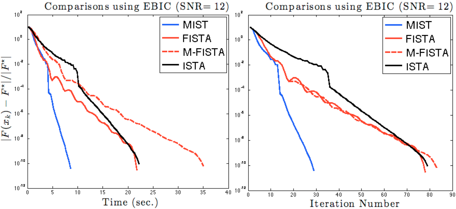
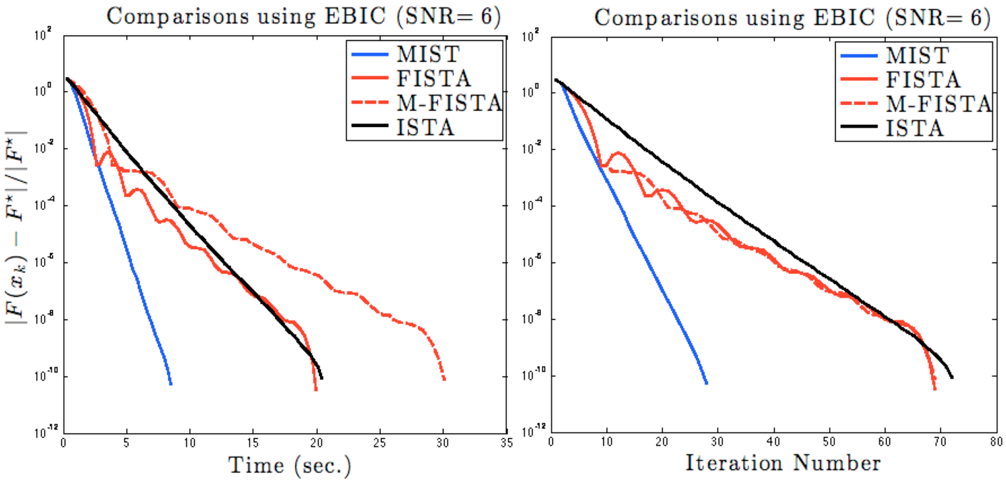
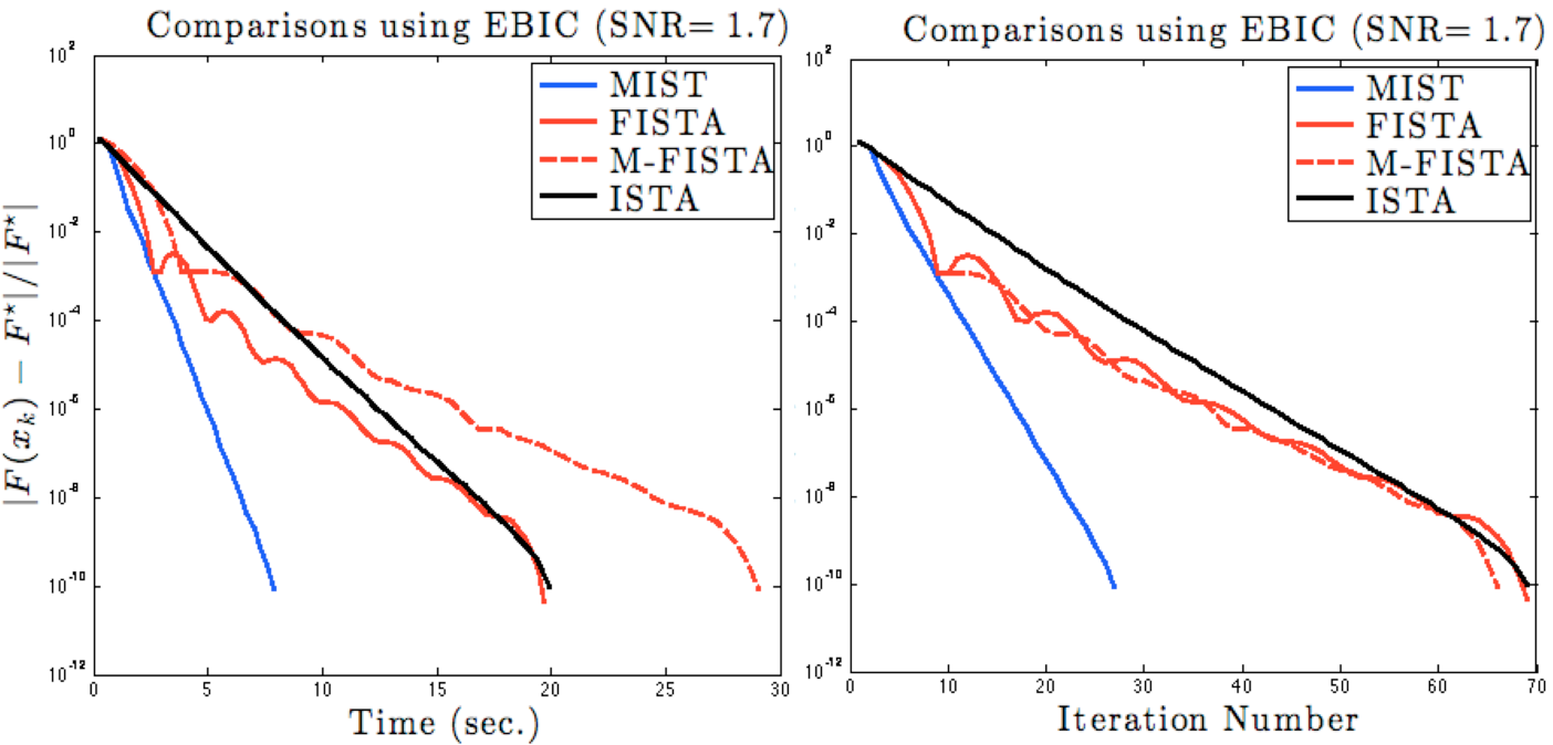
Figures 6, 6 and 6 show percentage reduction of F⁡(⋅)F(\cdot) as a function of time and iteration for each algorithm. To make the comparisons fair, i.e., to make sure all the algorithms minimize the same objective function, a common λ\lambda is used and chosen to be the smallest λ\lambda from the averaged arg⁡minλ​EBIC​(λ)\arg\min_{\lambda}\textup{EBIC}(\lambda) obtained by each algorithm (over 1010 instances).

Refer to caption
Fig. 4: Algorithm comparisons based on relative error |F⁡(𝐱k)−F⋆|/|F⋆||F(\mathbf{x}_{k})-F^{\star}|/|F^{\star}| where F⋆F^{\star} is the final value of F⁡(⋅)F(\cdot) obtained by each algorithm at its termination, i.e., F⋆=F⁡(𝐱k)F^{\star}=F(\mathbf{x}_{k}), where F⁡(𝐱k)F(\mathbf{x}_{k}) satisfies the termination criterion in (15). Here SNR=12, and the regularization parameter λ\lambda has been selected using the EBIC criterion. As it can be seen, in the low noise environment (σ=3)(\sigma=3) the MIST algorithm outperforms the rest, both in terms of time and iteration number.
Refer to caption
Fig. 5: Similar comparisons as in Fig. 6 except that SNR=6. As it can be seen, in the intermediate noise environment (σ=6)(\sigma=6) the MIST algorithm outperforms the others, both in terms of time and iteration number.
Refer to caption
Fig. 6: Similar comparisons as in Fig. 6 except that SNR=1.7. As it can be seen, in the high noise environment (σ=10)(\sigma=10) the MIST algorithm outperforms the rest, both in terms of time and iteration number.

Figures 9, 9 and 9 also show percentage reduction of F⁡(⋅)F(\cdot) as a function of time and iteration for each algorithm. This time the MSE is used for the tuning of λ\lambda, and again, to make sure all the algorithms minimize the same objective function, a common λ\lambda is used and chosen to be the smallest λ\lambda from the averaged arg⁡minλ​MSE​(λ)\arg\min_{\lambda}\textup{MSE}(\lambda) obtained by each algorithm (over 1010 instances).

Refer to caption
Fig. 7: Algorithm comparisons based on relative error |F⁡(𝐱k)−F⋆|/|F⋆||F(\mathbf{x}_{k})-F^{\star}|/|F^{\star}| where F⋆F^{\star} is the final value of F⁡(⋅)F(\cdot) obtained by each algorithm at its termination, i.e., F⋆=F⁡(𝐱k)F^{\star}=F(\mathbf{x}_{k}), where F⁡(𝐱k)F(\mathbf{x}_{k}) satisfies the termination criterion in (15). Here an oracle selects the regularization parameter λ\lambda using the minimum MSE criterion. As it can be seen, in the low noise environment (σ=3)(\sigma=3) the MIST algorithm outperforms the rest, both in terms of time and iteration number.
Refer to caption
Fig. 8: Similar comparisons as in Fig. 9 except that SNR=6. As it can be seen, in the intermediate noise environment (σ=6)(\sigma=6) the MIST algorithm outperforms the rest, both in terms of time and iteration number.
Refer to caption
Fig. 9: Similar comparisons as in Fig. 9 except that SNR=1.7. As it can be seen, in the high noise environment (σ=10)(\sigma=10) the MIST algorithm outperforms the rest, both in terms of time and iteration number.

Based on a large number of experiments we noticed that MIST, FISTA and ISTA outperformed M-FISTA in terms of run time. This could be due to the fact that M-FISTA requires computing a larger number of products, see Remark 1, and the fact that it is a monotone version of a severely non-monotone FISTA. The high non-monotonicity could possibly be due to non-convexity of the objective function F⁡(⋅)F(\cdot).

Lastly, Figures 12, 12 and 12 show the average speed of each algorithm as a function of λ\lambda.

Refer to caption
Fig. 10: Average time vs. λ\lambda over 55 instances when SNR=12. For the comparison, 2020 equally spaced values of λ\lambda are considered, where 10−4​‖𝐀T​𝐲‖∞≤λ≤0.2​‖𝐀T​𝐲‖∞10^{-4}\|\mathbf{A}^{T}\mathbf{y}\|_{\infty}\leq\lambda\leq 0.2\|\mathbf{A}^{T}\mathbf{y}\|_{\infty}. As it can be seen, except in the scenario when λ=10−4​‖𝐀T​𝐲‖∞\lambda=10^{-4}\|\mathbf{A}^{T}\mathbf{y}\|_{\infty} the MIST algorithm outperforms the others.
Refer to caption
Fig. 11: Similar comparisons as in Fig. 12 except that SNR=6. As it can be seen, except in the scenario when λ=10−4​‖𝐀T​𝐲‖∞\lambda=10^{-4}\|\mathbf{A}^{T}\mathbf{y}\|_{\infty} the MIST algorithm outperforms the others.
Refer to caption
Fig. 12: Similar comparisons as in Fig. 12 except that SNR=1.7. As it can be seen, except in the scenario when λ=10−4​‖𝐀T​𝐲‖∞\lambda=10^{-4}\|\mathbf{A}^{T}\mathbf{y}\|_{\infty} the MIST algorithm outperforms the others.

VI Conclusion

We have developed a momentum accelerated MM algorithm, MIST, for minimizing the l0l_{0} penalized least squares criterion for linear regression problems. We have proved that MIST converges to a local minimizer without imposing any assumptions on the regression matrix 𝐀\mathbf{A}. Simulations on large data sets were carried out for different SNR values, and have shown that the MIST algorithm outperforms other popular MM algorithms in terms of time and iteration number.

VII Appendix

Proof of Theorem 1: Let 𝐰=𝐱+β​𝜹\mathbf{w}=\mathbf{x}+\beta\bm{\delta}. The quantities f⁡(𝐰)f(\mathbf{w}), ∇f(𝐰)T(𝐳−𝐰)\nabla f(\mathbf{w})^{T}(\mathbf{z}-\mathbf{w}) and ‖𝐳−𝐰‖22\|\mathbf{z}-\mathbf{w}\|_{2}^{2} are quadratic functions, and by simple linear algebra they can easily be expanded in terms of 𝐳\mathbf{z}, 𝐱\mathbf{x} and 𝜹\bm{\delta}. Namely,

f⁡(𝐰)\displaystyle f(\mathbf{w}) =12​‖𝐀𝐰−𝐲‖2\displaystyle=\frac{1}{2}\|\mathbf{A}\mathbf{w}-\mathbf{y}\|^{2}
=12​‖𝐀𝐱−𝐲+β​𝐀​𝜹‖2\displaystyle=\frac{1}{2}\|\mathbf{A}\mathbf{x}-\mathbf{y}+\beta\mathbf{A}\bm{\delta}\|^{2}
=f⁡(𝐱)+β​(𝐀𝐱−𝐲)T​𝐀​𝜹+12​β2​‖𝐀​𝜹‖2\displaystyle=f(\mathbf{x})+\beta(\mathbf{A}\mathbf{x}-\mathbf{y})^{T}\mathbf{A}\bm{\delta}+\frac{1}{2}\beta^{2}\|\mathbf{A}\bm{\delta}\|^{2}
=f(𝐱)+β∇f(𝐱)T𝜹+12β2∥𝐀𝜹∥2.\displaystyle=f(\mathbf{x})+\beta\nabla f(\mathbf{x})^{T}\bm{\delta}+\frac{1}{2}\beta^{2}\|\mathbf{A}\bm{\delta}\|^{2}. (16)

Also,

∇f(𝐰)T(𝐳−𝐰)\displaystyle\nabla f(\mathbf{w})^{T}(\mathbf{z}-\mathbf{w})
=(∇f​(𝐱)+β​𝐀T​𝐀​𝜹)T​(𝐳−𝐰)\displaystyle=(\nabla f(\mathbf{x})+\beta\mathbf{A}^{T}\mathbf{A}\bm{\delta})^{T}(\mathbf{z}-\mathbf{w})
=∇f(𝐱)T(𝐳−𝐰)+β𝜹T𝐀T𝐀(𝐳−𝐰)\displaystyle=\nabla f(\mathbf{x})^{T}(\mathbf{z}-\mathbf{w})+\beta\bm{\delta}^{T}\mathbf{A}^{T}\mathbf{A}(\mathbf{z}-\mathbf{w})
=∇f(𝐱)T(𝐳−𝐱−β𝜹)+β𝜹T𝐀T𝐀(𝐳−𝐱−β𝜹)\displaystyle=\nabla f(\mathbf{x})^{T}(\mathbf{z}-\mathbf{x}-\beta\bm{\delta})+\beta\bm{\delta}^{T}\mathbf{A}^{T}\mathbf{A}(\mathbf{z}-\mathbf{x}-\beta\bm{\delta})
=∇f(𝐱)T(𝐳−𝐱)−β∇f(𝐱)T𝜹+β𝜹T𝐀T𝐀(𝐳−𝐱)\displaystyle=\nabla f(\mathbf{x})^{T}(\mathbf{z}-\mathbf{x})-\beta\nabla f(\mathbf{x})^{T}\bm{\delta}+\beta\bm{\delta}^{T}\mathbf{A}^{T}\mathbf{A}(\mathbf{z}-\mathbf{x})
−β2​‖𝐀​𝜹‖2,\displaystyle\hskip 14.22636pt-\beta^{2}\|\mathbf{A}\bm{\delta}\|^{2}, (17)

and finally:

‖𝐳−𝐰‖22\displaystyle\|\mathbf{z}-\mathbf{w}\|_{2}^{2} =‖𝐳−𝐱−β​𝜹‖22\displaystyle=\|\mathbf{z}-\mathbf{x}-\beta\bm{\delta}\|_{2}^{2}
=‖𝐳−𝐱‖22−β​𝜹T​(𝐳−𝐱)+β2​‖𝜹‖22\displaystyle=\|\mathbf{z}-\mathbf{x}\|_{2}^{2}-\beta\bm{\delta}^{T}(\mathbf{z}-\mathbf{x})+\beta^{2}\|\bm{\delta}\|_{2}^{2} (18)

Using the above expansions and the definition of Qμ​(⋅,⋅)Q_{\mu}(\cdot,\cdot), we have that:

Qμ​(𝐳,𝐰)=Qμ​(𝐳,𝐱)+Φμ​(𝐳,𝜹,β),\displaystyle Q_{\mu}(\mathbf{z},\mathbf{w})=Q_{\mu}(\mathbf{z},\mathbf{x})+\Phi_{\mu}(\mathbf{z},\bm{\delta},\beta), (19)

where:

Φμ​(𝐳,𝜹,β)=12​β2​𝜹T​𝐁μ​𝜹−β​𝜹T​𝐁μ​(𝐳−𝐱).\displaystyle\Phi_{\mu}(\mathbf{z},\bm{\delta},\beta)=\frac{1}{2}\beta^{2}\bm{\delta}^{T}\mathbf{B}_{\mu}\bm{\delta}-\beta\bm{\delta}^{T}\mathbf{B}_{\mu}(\mathbf{z}-\mathbf{x}).

Observing that 𝜹T​𝐁μ​𝜹>0\bm{\delta}^{T}\mathbf{B}_{\mu}\bm{\delta}>0, let:

β=2​η​(𝜹T​𝐁μ​(𝐳−𝐱)𝜹T​𝐁μ​𝜹),η∈[0,1].\displaystyle\beta=2\eta\left(\frac{\bm{\delta}^{T}\mathbf{B}_{\mu}(\mathbf{z}-\mathbf{x})}{\bm{\delta}^{T}\mathbf{B}_{\mu}\bm{\delta}}\right),\ \eta\in[0,1]. (20)

Then, one has:

Qμ​(𝒫μ​(𝐰),𝐰)\displaystyle\hskip-5.69054ptQ_{\mu}(\mathcal{P}_{\mu}(\mathbf{w}),\mathbf{w}) =min𝐳⁡Qμ​(𝐳,𝐰)≤Qμ​(𝐳,𝐰)\displaystyle=\min_{\mathbf{z}}Q_{\mu}(\mathbf{z},\mathbf{w})\leq Q_{\mu}(\mathbf{z},\mathbf{w})
=(19)​Qμ​(𝐳,𝐱)+Φμ​(𝐳,𝜹,β)\displaystyle\overset{(\ref{expansion of Q})}{=}Q_{\mu}(\mathbf{z},\mathbf{x})+\Phi_{\mu}(\mathbf{z},\bm{\delta},\beta)
=(20)​Qμ​(𝐳,𝐱)−2​η​(1−η)​[𝜹T​𝐁μ​(𝐳−𝐱)]2𝜹T​𝐁μ​𝜹\displaystyle\overset{(\ref{beta expression})}{=}Q_{\mu}(\mathbf{z},\mathbf{x})-2\eta(1-\eta)\frac{[\bm{\delta}^{T}\mathbf{B}_{\mu}(\mathbf{z}-\mathbf{x})]^{2}}{\bm{\delta}^{T}\mathbf{B}_{\mu}\bm{\delta}} (21)
≤Qμ​(𝐳,𝐱),\displaystyle\leq Q_{\mu}(\mathbf{z},\mathbf{x}), (22)

which holds for any 𝐳\mathbf{z}. So, letting 𝐳=𝒫μ​(𝐱)\mathbf{z}=\mathcal{P}_{\mu}(\mathbf{x}) implies:

F⁡(𝒫μ​(𝐰))​≤(5)​Qμ​(𝒫μ​(𝐰),𝐰)​≤(22)​Qμ​(𝒫μ​(𝐱),𝐱)​≤(5)​F​(𝐱),\displaystyle F(\mathcal{P}_{\mu}(\mathbf{w}))\overset{(\ref{Fxkp<=Fxk})}{\leq}Q_{\mu}(\mathcal{P}_{\mu}(\mathbf{w}),\mathbf{w})\overset{(\ref{Qm inequality})}{\leq}Q_{\mu}(\mathcal{P}_{\mu}(\mathbf{x}),\mathbf{x})\overset{(\ref{Fxkp<=Fxk})}{\leq}F(\mathbf{x}),

which completes the proof. ∎

Proof of Theorem 2: Looking at (8) it is obvious that:

𝒫μ​(𝐯)​[i]=arg⁡min𝐳⁡[i]​12​(𝐳⁡[i]−g⁡(𝐯)​[i])2+(λ/μ)​𝕀​(𝐳⁡[i]≠0).\displaystyle\mathcal{P}_{\mu}(\mathbf{v})[i]=\arg\min_{\mathbf{z}[i]}\frac{1}{2}(\mathbf{z}[i]-g(\mathbf{v})[i])^{2}+(\lambda/\mu)\mathbb{I}(\mathbf{z}[i]\neq 0).

If |g​(𝐯)​[i]|≠2​λ/μ|g(\mathbf{v})[i]|\neq\sqrt{2\lambda/\mu}, by [22, Theorem 1] 𝒫μ​(𝐯)​[i]\mathcal{P}_{\mu}(\mathbf{v})[i] is unique and given by ℋλ/μ​(g​(𝐯))​[i]\mathcal{H}_{\lambda/\mu}(g(\mathbf{v}))[i]. If |g​(𝐯)​[i]|=2​λ/μ|g(\mathbf{v})[i]|=\sqrt{2\lambda/\mu}, again by [22, Theorem 1] we now have:

𝒫μ​(𝐯)​[i]=0​ and ​𝒫μ​(𝐯)​[i]=sgn​(g⁡(𝐯)​[i])​2​λ/μ.\displaystyle\mathcal{P}_{\mu}(\mathbf{v})[i]=0\textup{ and }\mathcal{P}_{\mu}(\mathbf{v})[i]=\textup{sgn}(g(\mathbf{v})[i])\sqrt{2\lambda/\mu}.

Hence, ℋλ/μ​(g⁡(𝐯))​[i]∈𝒫μ​(𝐯)​[i]\mathcal{H}_{\lambda/\mu}(g(\mathbf{v}))[i]\in\mathcal{P}_{\mu}(\mathbf{v})[i], completing the proof. ∎

Proof of Lemma 1: From Theorem 1, 0≤F⁡(𝐱k+1)≤F⁡(𝐱k)0\leq F(\mathbf{x}_{k+1})\leq F(\mathbf{x}_{k}), so the sequence {F⁡(𝐱k)}k≥0\{F(\mathbf{x}_{k})\}_{k\geq 0} is bounded, which means it has a finite limit, say, F∙F_{\bullet}. As a result:

F⁡(𝐱k)−F⁡(𝐱k+1)→F∙−F∙=0.\displaystyle F(\mathbf{x}_{k})-F(\mathbf{x}_{k+1})\to F_{\bullet}-F_{\bullet}=0. (23)

Next, recall that 𝐰k=𝐱k+αk​𝜹k\mathbf{w}_{k}=\mathbf{x}_{k}+\alpha_{k}\bm{\delta}_{k} and g(⋅)=(⋅)−1μ∇f(⋅)g(\cdot)=(\cdot)-\frac{1}{\mu}\nabla f(\cdot). So, using (21) in the proof of Theorem 1 (where 𝐳=𝒫μ​(𝐱)\mathbf{z}=\mathcal{P}_{\mu}(\mathbf{x})) with 𝐰\mathbf{w}, 𝒫μ​(𝐰)\mathcal{P}_{\mu}(\mathbf{w}), 𝒫μ​(⋅)\mathcal{P}_{\mu}(\cdot), 𝐱\mathbf{x}, and 𝜹\bm{\delta} respectively replaced by 𝐰k\mathbf{w}_{k}, 𝐱k+1\mathbf{x}_{k+1}, ℋλ/μ​(g​(⋅))\mathcal{H}_{\lambda/\mu}(g(\cdot)), 𝐱k\mathbf{x}_{k} and 𝜹k\bm{\delta}_{k}, we have:

Qμ​(𝐱k+1,𝐰k)\displaystyle Q_{\mu}(\mathbf{x}_{k+1},\mathbf{w}_{k}) ≤Qμ​(ℋλ/μ​(g⁡(𝐱k)),𝐱k)\displaystyle\leq Q_{\mu}(\mathcal{H}_{\lambda/\mu}(g(\mathbf{x}_{k})),\mathbf{x}_{k})
−2​ηk​(1−ηk)​[𝜹kT​𝐁μ​(ℋλ/μ​(g⁡(𝐱k))−𝐱k)]2𝜹k​𝐁μ​𝜹k\displaystyle-2\eta_{k}(1-\eta_{k})\frac{[\bm{\delta}_{k}^{T}\mathbf{B}_{\mu}(\mathcal{H}_{\lambda/\mu}(g(\mathbf{x}_{k}))-\mathbf{x}_{k})]^{2}}{\bm{\delta}_{k}\mathbf{B}_{\mu}\bm{\delta}_{k}}
≤F⁡(𝐱k)−σk​αk2​𝜹kT​𝐁μ​𝜹k,\displaystyle\leq F(\mathbf{x}_{k})-\sigma_{k}\alpha_{k}^{2}\bm{\delta}_{k}^{T}\mathbf{B}_{\mu}\bm{\delta}_{k}, (24)

where σk=(1−ηk)/2​ηk>0\sigma_{k}=(1-\eta_{k})/2\eta_{k}>0. The first term in (24) follows from the fact that:

Qμ​(ℋλ/μ​(g⁡(𝐱k)),𝐱k)=Qμ​(𝒫μ​(𝐱k),𝐱k)≤F⁡(𝐱k).\displaystyle Q_{\mu}(\mathcal{H}_{\lambda/\mu}(g(\mathbf{x}_{k})),\mathbf{x}_{k})=Q_{\mu}(\mathcal{P}_{\mu}(\mathbf{x}_{k}),\mathbf{x}_{k})\leq F(\mathbf{x}_{k}).

Now, noting that:

Qμ​(𝐱k+1,𝐰k)\displaystyle Q_{\mu}(\mathbf{x}_{k+1},\mathbf{w}_{k}) =F⁡(𝐱k+1)\displaystyle=F(\mathbf{x}_{k+1})
+12​(𝐱k+1−𝐰k)T​𝐁μ​(𝐱k+1−𝐰k),\displaystyle+\frac{1}{2}(\mathbf{x}_{k+1}-\mathbf{w}_{k})^{T}\mathbf{B}_{\mu}(\mathbf{x}_{k+1}-\mathbf{w}_{k}), (25)

which easily follows from basic linear algebra, (24) and (25) together imply that:

F⁡(𝐱k)−F⁡(𝐱k+1)\displaystyle\hskip-5.69054ptF(\mathbf{x}_{k})-F(\mathbf{x}_{k+1}) ≥σk​αk2​𝜹kT​𝐁μ​𝜹k\displaystyle\geq\sigma_{k}\alpha_{k}^{2}\bm{\delta}_{k}^{T}\mathbf{B}_{\mu}\bm{\delta}_{k}
+12​(𝐱k+1−𝐰k)T​𝐁μ​(𝐱k+1−𝐰k)\displaystyle+\frac{1}{2}(\mathbf{x}_{k+1}-\mathbf{w}_{k})^{T}\mathbf{B}_{\mu}(\mathbf{x}_{k+1}-\mathbf{w}_{k})
≥ρ​σk​αk2​‖𝜹k‖22+ρ2​‖𝐱k+1−𝐰k‖22,\displaystyle\geq\rho\sigma_{k}\alpha_{k}^{2}\|\bm{\delta}_{k}\|_{2}^{2}+\frac{\rho}{2}\|\mathbf{x}_{k+1}-\mathbf{w}_{k}\|_{2}^{2}, (26)

where ρ>0\rho>0 is the smallest eigenvalue of 𝐁μ≻0\mathbf{B}_{\mu}\succ 0. So, both terms on the right hand side in (26) are ≥0\geq 0 for all kk. As a result, due to (23) we can use the pinching/squeeze argument on (26) to establish that 𝐱k+1−𝐰k=𝜹k+1−αk​𝜹k→0\mathbf{x}_{k+1}-\mathbf{w}_{k}=\bm{\delta}_{k+1}-\alpha_{k}\bm{\delta}_{k}\to 0 and αk​𝜹k→0\alpha_{k}\bm{\delta}_{k}\to 0 as k→∞k\to\infty. Consequently, 𝜹k→0\bm{\delta}_{k}\to 0 as k→∞k\to\infty, which completes the proof. ∎

Proof of Lemma 2: Firstly, from Lemma 1 we have that 𝐱kn−𝐱kn−1→0\mathbf{x}_{k_{n}}-\mathbf{x}_{k_{n}-1}\to 0 as n→∞n\to\infty. In the last paragraph in the proof of that lemma (above) we also have that αk​𝜹k→0\alpha_{k}\bm{\delta}_{k}\to 0, and so, αkn​𝜹kn→0\alpha_{k_{n}}\bm{\delta}_{k_{n}}\to 0 as n→∞n\to\infty. As a result, by the definition of 𝐰kn\mathbf{w}_{k_{n}}, 𝐰kn→𝐰∙=𝐱∙\mathbf{w}_{k_{n}}\to\mathbf{w}_{\bullet}=\mathbf{x}_{\bullet}. Then, by the continuity of ∇f​(⋅)\nabla f(\cdot) we have that:

𝐰kn−1μ∇f(𝐰kn)→𝐱∙−1μ∇f(𝐱∙).\displaystyle\mathbf{w}_{k_{n}}-\frac{1}{\mu}\nabla f(\mathbf{w}_{k_{n}})\to\mathbf{x}_{\bullet}-\frac{1}{\mu}\nabla f(\mathbf{x}_{\bullet}).

Now, we need to show that, if 𝐮kn→𝐮∙\mathbf{u}_{k_{n}}\to\mathbf{u}_{\bullet} as n→∞n\to\infty, then:

ℋλ/μ​(𝐮kn)→ℋλ/μ​(𝐮∙).\displaystyle\mathcal{H}_{\lambda/\mu}(\mathbf{u}_{k_{n}})\to\mathcal{H}_{\lambda/\mu}(\mathbf{u}_{\bullet}). (27)

Consider an arbitrary component of 𝐮kn\mathbf{u}_{k_{n}}, say, 𝐮kn​[i]\mathbf{u}_{k_{n}}[i], in which case we must have 𝐮kn​[i]→𝐮∙​[i]\mathbf{u}_{k_{n}}[i]\to\mathbf{u}_{\bullet}[i]. Without loss of generality, assume 𝐮∙​[i]>0\mathbf{u}_{\bullet}[i]>0. Then, by the definition of ℋλ/μ​(⋅)\mathcal{H}_{\lambda/\mu}(\cdot), there are two scenarios to consider:

(a)​𝐮∙​[i]≠2​λ/μ(b)​𝐮∙​[i]=2​λ/μ.\displaystyle\textup{(a)}\hskip 5.69054pt\mathbf{u}_{\bullet}[i]\neq\sqrt{2\lambda/\mu}\hskip 28.45274pt\textup{(b)}\hskip 5.69054pt\mathbf{u}_{\bullet}[i]=\sqrt{2\lambda/\mu}.

Regarding (a): For a large enough n=Nn=N, we must either have 𝐮kn​[i]<2​λ/μ\mathbf{u}_{k_{n}}[i]<\sqrt{2\lambda/\mu} or 𝐮kn​[i]>2​λ/μ\mathbf{u}_{k_{n}}[i]>\sqrt{2\lambda/\mu} for all n>Nn>N, which implies:

ℋλ/μ​(𝐮kn)​[i]={0if ​𝐮kn​[i]<2​λ/μ𝐮kn​[i]if ​𝐮kn​[i]>2​λ/μ,\displaystyle\mathcal{H}_{\lambda/\mu}(\mathbf{u}_{k_{n}})[i]=\begin{cases}0&\textup{if }\mathbf{u}_{k_{n}}[i]<\sqrt{2\lambda/\mu}\\[5.69054pt] \mathbf{u}_{k_{n}}[i]&\textup{if }\mathbf{u}_{k_{n}}[i]>\sqrt{2\lambda/\mu},\end{cases} (28)

for all n>Nn>N. In (28), ℋλ/μ​(⋅)\mathcal{H}_{\lambda/\mu}(\cdot) is a continuous function of 𝐮kn​[i]\mathbf{u}_{k_{n}}[i] in both cases, which immediately implies (27).

Regarding (b): In general, 𝐮∙​[i]\mathbf{u}_{\bullet}[i] could be reached in an oscillating fashion, i.e., for some nn we can have 𝐮kn​[i]<2​λ/μ\mathbf{u}_{k_{n}}[i]<\sqrt{2\lambda/\mu} and for others 𝐮kn​[i]>2​λ/μ\mathbf{u}_{k_{n}}[i]>\sqrt{2\lambda/\mu}. If this was the case for all n→∞n\to\infty then ℋλ/μ​(𝐮kn)​[i]\mathcal{H}_{\lambda/\mu}(\mathbf{u}_{k_{n}})[i] would approach a limit set of two points {0,2​λ/μ}\{0,\sqrt{2\lambda/\mu}\}. However, having 𝐱kn→𝐱∙\mathbf{x}_{k_{n}}\to\mathbf{x}_{\bullet} and 𝐱k+1−𝐱k→0\mathbf{x}_{k+1}-\mathbf{x}_{k}\to 0 implies 𝐱kn+1→𝐱∙\mathbf{x}_{k_{n}+1}\to\mathbf{x}_{\bullet}. So, using the fact that:

𝐱kn+1​[i]=ℋλ/μ​(𝐮kn)​[i]\displaystyle\mathbf{x}_{k_{n}+1}[i]=\mathcal{H}_{\lambda/\mu}(\mathbf{u}_{k_{n}})[i] (29)

ℋλ/μ​(𝐮kn)​[i]\mathcal{H}_{\lambda/\mu}(\mathbf{u}_{k_{n}})[i] must approach either 00 or 2​λ/μ\sqrt{2\lambda/\mu}. In other words, there has to exist a large enough n=Nn=N such that 𝐮∙​[i]\mathbf{u}_{\bullet}[i] is approached either only from the left or the right for all n>Nn>N, i.e.,

  • (b1)

    if 𝐮kn​[i]<𝐮∙​[i]=2​λ/μ\mathbf{u}_{k_{n}}[i]<\mathbf{u}_{\bullet}[i]=\sqrt{2\lambda/\mu} for all n>Nn>N, from (28) we have ℋλ/μ​(𝐮kn)​[i]→0\mathcal{H}_{\lambda/\mu}(\mathbf{u}_{k_{n}})[i]\to 0. So, noting that:

    ℋλ/μ​(𝐮kn)​[i]−𝐱kn​=(29)​𝐱kn+1−𝐱kn→0\displaystyle\mathcal{H}_{\lambda/\mu}(\mathbf{u}_{k_{n}})[i]-\mathbf{x}_{k_{n}}\overset{(\ref{xkp=H})}{=}\mathbf{x}_{k_{n}+1}-\mathbf{x}_{k_{n}}\to 0 (30)

    implies 𝐱kn​[i]→0\mathbf{x}_{k_{n}}[i]\to 0. As a result, 𝐱∙​[i]=0\mathbf{x}_{\bullet}[i]=0, and using the definition of ℋλ/μ​(⋅)\mathcal{H}_{\lambda/\mu}(\cdot), we have:

    ℋλ/μ​(𝐮∙)​[i]\displaystyle\mathcal{H}_{\lambda/\mu}(\mathbf{u}_{\bullet})[i] =2​λ/μ​𝕀​(𝐰∙​[i]≠0)\displaystyle=\sqrt{2\lambda/\mu}\ \mathbb{I}(\mathbf{w}_{\bullet}[i]\neq 0)
    =2​λ/μ​𝕀​(𝐱∙​[i]≠0)=2​λ/μ⋅0\displaystyle=\sqrt{2\lambda/\mu}\ \mathbb{I}(\mathbf{x}_{\bullet}[i]\neq 0)=\sqrt{2\lambda/\mu}\cdot 0
    =0.\displaystyle=0.

    Hence, (27) is satisfied.

  • (b2)

    if 𝐮kn​[i]>𝐮∙​[i]=2​λ/μ\mathbf{u}_{k_{n}}[i]>\mathbf{u}_{\bullet}[i]=\sqrt{2\lambda/\mu} for all n>Nn>N, from (28) we have ℋλ/μ​(𝐮kn)​[i]→2​λ/μ\mathcal{H}_{\lambda/\mu}(\mathbf{u}_{k_{n}})[i]\to\sqrt{2\lambda/\mu}. So, (30) implies 𝐱kn→2​λ/μ\mathbf{x}_{k_{n}}\to\sqrt{2\lambda/\mu}, and using the definition of ℋλ/μ​(⋅)\mathcal{H}_{\lambda/\mu}(\cdot), we have:

    ℋλ/μ​(𝐮∙)​[i]\displaystyle\mathcal{H}_{\lambda/\mu}(\mathbf{u}_{\bullet})[i] =2​λ/μ​𝕀​(𝐰∙​[i]≠0)\displaystyle=\sqrt{2\lambda/\mu}\ \mathbb{I}(\mathbf{w}_{\bullet}[i]\neq 0)
    =2​λ/μ​𝕀​(𝐱∙​[i]≠0)=2​λ/μ⋅1\displaystyle=\sqrt{2\lambda/\mu}\ \mathbb{I}(\mathbf{x}_{\bullet}[i]\neq 0)=\sqrt{2\lambda/\mu}\cdot 1
    =2​λ/μ.\displaystyle=\sqrt{2\lambda/\mu}.

    Hence, (27) is again satisfied.

Since ii is arbitrary, the proof is complete. ∎

Proof of Lemma 3: The fixed points are obviously obtained by setting 𝐱k+1=𝐱k=𝐱k−1=𝐱∙\mathbf{x}_{k+1}=\mathbf{x}_{k}=\mathbf{x}_{k-1}=\mathbf{x}_{\bullet}. So, any fixed point 𝐱∙\mathbf{x}_{\bullet} satisfies the equation:

𝐱∙=ℋλ/μ(𝐱∙−1μ∇f(𝐱∙)).\displaystyle\mathbf{x}_{\bullet}=\mathcal{H}_{\lambda/\mu}\left(\mathbf{x}_{\bullet}-\frac{1}{\mu}\nabla f(\mathbf{x}_{\bullet})\right). (31)

The result is established by using the definition of ℋλ/μ​(g​(⋅))\mathcal{H}_{\lambda/\mu}(g(\cdot)) in Theorem 2. Namely, if i∈𝒵i\in\mathcal{Z} we easily obtain:

|(1/μ)∇f(𝐱∙)[i]|≤2​λ/μ,\displaystyle|(1/\mu)\nabla f(\mathbf{x}_{\bullet})[i]|\leq\sqrt{2\lambda/\mu},

which reduces to C1. If i∈𝒵ci\in\mathcal{Z}^{c}, we easily obtain:

𝐱∙[i]=𝐱∙[i]−(1/μ)∇f(𝐱∙)[i],\displaystyle\mathbf{x}_{\bullet}[i]=\mathbf{x}_{\bullet}[i]-(1/\mu)\nabla f(\mathbf{x}_{\bullet})[i], (32)

which reduces to C2. However, since:

|𝐱∙[i]−(1/μ)∇f(𝐱∙)[i]|≥2​λ/μ,\displaystyle\left|\mathbf{x}_{\bullet}[i]-(1/\mu)\nabla f(\mathbf{x}_{\bullet})[i]\right|\geq\sqrt{2\lambda/\mu}, (33)

(32) and (33) together imply |𝐱∙​[i]|≥2​λ/μ|\mathbf{x}_{\bullet}[i]|\geq\sqrt{2\lambda/\mu}, giving C3. ∎

Proof of Lemma 4: Letting 𝒵={i:𝐱∙​[i]=0}\mathcal{Z}=\{i:\mathbf{x}_{\bullet}[i]=0\} and 𝒵c={i:𝐱∙​[i]≠0}\mathcal{Z}^{c}=\{i:\mathbf{x}_{\bullet}[i]\neq 0\}, it can easily be shown that F⁡(𝐱∙+𝐝)=F⁡(𝐱∙)+ϕ⁡(𝐝)F(\mathbf{x}_{\bullet}+\mathbf{d})=F(\mathbf{x}_{\bullet})+\phi(\mathbf{d}), where:

ϕ⁡(𝐝)\displaystyle\phi(\mathbf{d}) =12∥𝐀𝐝∥22+𝐝T∇f(𝐱∙)+λ∥𝐱∙+𝐝∥0−λ∥𝐱∙∥0\displaystyle=\frac{1}{2}\|\mathbf{A}\mathbf{d}\|_{2}^{2}+\mathbf{d}^{T}\nabla f(\mathbf{x}_{\bullet})+\lambda\|\mathbf{x}_{\bullet}+\mathbf{d}\|_{0}-\lambda\|\mathbf{x}_{\bullet}\|_{0}
≥∑i∈𝒵𝐝[i]∇f(𝐱∙)[i]+λ𝕀(𝐝[i]≠0)⏟=ϕ𝒵​(𝐝​[i])\displaystyle\geq\sum_{i\in\mathcal{Z}}\underbrace{\mathbf{d}[i]\nabla f(\mathbf{x}_{\bullet})[i]+\lambda\mathbb{I}(\mathbf{d}[i]\neq 0)}_{=\phi_{\mathcal{Z}}(\mathbf{d}[i])}
+∑i∈𝒵c𝐝[i]∇f(𝐱∙)[i]+λ𝕀(𝐱∙[i]+𝐝[i]≠0)−λ⏟=ϕ𝒵c​(𝐝​[i]).\displaystyle+\sum_{i\in\mathcal{Z}^{c}}\underbrace{\mathbf{d}[i]\nabla f(\mathbf{x}_{\bullet})[i]+\lambda\mathbb{I}(\mathbf{x}_{\bullet}[i]+\mathbf{d}[i]\neq 0)-\lambda}_{=\phi_{\mathcal{Z}^{c}}(\mathbf{d}[i])}.

Now, ϕ𝒵​(0)=0\phi_{\mathcal{Z}}(0)=0, so suppose |𝐝⁡[i]|∈(0,λ/2​λ​μ)|\mathbf{d}[i]|\in\left(0,\lambda/\sqrt{2\lambda\mu}\right), i∈𝒵i\in\mathcal{Z}. Then:

ϕ𝒵​(𝐝⁡[i])≥−|𝐝⁡[i]|​|∇f​(𝐱∙)​[i]|+λ≥−|𝐝⁡[i]|​2​λ​μ+λ>0.\displaystyle\phi_{\mathcal{Z}}(\mathbf{d}[i])\geq-|\mathbf{d}[i]||\nabla f(\mathbf{x}_{\bullet})[i]|+\lambda\geq-|\mathbf{d}[i]|\sqrt{2\lambda\mu}+\lambda>0.

The second inequality in the above is due to C1 in Lemma 3.

Lastly, note that ϕ𝒵c​(0)=0\phi_{\mathcal{Z}^{c}}(0)=0, and suppose i∈𝒵ci\in\mathcal{Z}^{c}. From C2 in Lemma 3 we have ∇f​(𝐱∙)​[i]=0\nabla f(\mathbf{x}_{\bullet})[i]=0. Thus, supposing |𝐝⁡[i]|∈(0,2​λ/μ)|\mathbf{d}[i]|\in(0,\sqrt{2\lambda/\mu}), from C2 we have |𝐝⁡[i]|<|𝐱∙​[i]||\mathbf{d}[i]|<|\mathbf{x}_{\bullet}[i]| for all i∈𝒵ci\in\mathcal{Z}^{c}. Thus:

𝕀⁡(𝐱∙​[i]+𝐝⁡[i]≠0)=𝕀⁡(𝐱∙​[i]≠0)=1,\displaystyle\mathbb{I}(\mathbf{x}_{\bullet}[i]+\mathbf{d}[i]\neq 0)=\mathbb{I}(\mathbf{x}_{\bullet}[i]\neq 0)=1,

and so, ϕ𝒵c​(𝐝​[i])=0\phi_{\mathcal{Z}^{c}}(\mathbf{d}[i])=0. Since λ2​λ​μ<2​λμ\frac{\lambda}{\sqrt{2\lambda\mu}}<\sqrt{\frac{2\lambda}{\mu}}, the proof is complete after letting ϵ=λ2​λ​μ\epsilon=\frac{\lambda}{\sqrt{2\lambda\mu}}. ∎

Proof of Lemma 5: Since it is assumed that {𝐱k}k≥0\{\mathbf{x}_{k}\}_{k\geq 0} is bounded, the sequence {(𝐱k,𝐱k+1)}k≥0\{(\mathbf{x}_{k},\mathbf{x}_{k+1})\}_{k\geq 0} is also bounded, and thus, has at least one limit point. Denoting one of these by (𝐱∙,𝐱∙⁣∙)(\mathbf{x}_{\bullet},\mathbf{x}_{\bullet\bullet}), there exists a subsequence {(𝐱kn,𝐱kn+1)}n≥0\{(\mathbf{x}_{k_{n}},\mathbf{x}_{k_{n}+1})\}_{n\geq 0} such that (𝐱kn,𝐱kn+1)→(𝐱∙,𝐱∙⁣∙)(\mathbf{x}_{k_{n}},\mathbf{x}_{k_{n}+1})\to(\mathbf{x}_{\bullet},\mathbf{x}_{\bullet\bullet}) as n→∞n\to\infty. However, by Lemma 1 we must have 𝐱kn−𝐱kn+1→0\mathbf{x}_{k_{n}}-\mathbf{x}_{k_{n}+1}\to 0, which implies 𝐱∙=𝐱∙⁣∙\mathbf{x}_{\bullet}=\mathbf{x}_{\bullet\bullet}. Consequently:

𝐱kn+1=ℋλ/μ(𝐰kn−1μ∇f(𝐰kn))→𝐱∙,\displaystyle\mathbf{x}_{k_{n}+1}=\mathcal{H}_{\lambda/\mu}\left(\mathbf{w}_{k_{n}}-\frac{1}{\mu}\nabla f(\mathbf{w}_{k_{n}})\right)\to\mathbf{x}_{\bullet}, (34)

recalling that 𝐰kn=𝐱kn+αkn​𝜹kn\mathbf{w}_{k_{n}}=\mathbf{x}_{k_{n}}+\alpha_{k_{n}}\bm{\delta}_{k_{n}} and 𝜹kn=𝐱kn−𝐱kn−1\bm{\delta}_{k_{n}}=\mathbf{x}_{k_{n}}-\mathbf{x}_{k_{n}-1}. Furthermore, the convergence:

ℋλ/μ(𝐰kn−1μ∇f(𝐰kn))→ℋλ/μ(𝐱∙−1μ∇f(𝐱∙)),\displaystyle\mathcal{H}_{\lambda/\mu}\left(\mathbf{w}_{k_{n}}-\frac{1}{\mu}\nabla f(\mathbf{w}_{k_{n}})\right)\to\mathcal{H}_{\lambda/\mu}\left(\mathbf{x}_{\bullet}-\frac{1}{\mu}\nabla f(\mathbf{x}_{\bullet})\right), (35)

follows from Lemma 2. Equating the limits in (34) and (35) assures that 𝐱∙\mathbf{x}_{\bullet} satisfies the fixed point equation (31), making it a fixed point of the algorithm. This completes the proof. ∎

Proof of Theorem 3: By Lemma 1 and Ostrowski’s result [23, Theorem 26.1], the bounded {𝐱k}k≥0\{\mathbf{x}_{k}\}_{k\geq 0} converges to a closed and connected set, i.e., the set of limit points form a closed and connected set. But, by Lemma 5 these limit points are fixed points, which by Lemma 4 are strict local minimizers. So, since the local minimizers form a discrete set the connected set of limit points can only contain one point, and so, the entire {𝐱k}k≥0\{\mathbf{x}_{k}\}_{k\geq 0} must converge to a single local minimizer. ∎

References

  • [1] T. Blumensath, M. Yaghoobi, and M. E. Davies, “Iterative hard thresholding and l0l_{0} regularisation,” IEEE ICASSP, vol. 3, pp. 877–880, 2007.
  • [2] T. Blumensath and M. Davies, “Iterative thresholding for sparse approximations,” J. Fourier Anal. Appl., vol. 14, no. 5, pp. 629–654, 2008.
  • [3] R. Mazumder, J. Friedman, and T. Hastie, “SparseNet: Coordinate descent with non-convex penalties,” J. Am. Stat. Assoc., vol. 106, no. 495, pp. 1–38, 2011.
  • [4] K. Bredies, D. A. Lorenz, and S. Reiterer, “Minimization of non-smooth, non-convex functionals by iterative thresholding,” Tech. Rept., 2009, http://www.uni-graz.at/~bredies/publications.html.
  • [5] P. Tseng, “Convergence of block coordinate descent method for nondifferentiable minimization,” J. Optimiz. Theory App., vol. 109, no. 3, pp. 474–494, 2001.
  • [6] M. Nikolova, “Description of the minimisers of least squares regularized with l0l_{0} norm. uniqueness of the global minimizer,” SIAM J. Imaging. Sci., vol. 6, no. 2, pp. 904–937, 2013.
  • [7] G. Marjanovic and V. Solo, “On exact lql_{q} denoising,” IEEE ICASSP, pp. 6068–6072, 2013.
  • [8] ——, “lql_{q} sparsity penalized linear regression with cyclic descent,” IEEE T. Signal Proces., vol. 62, no. 6, pp. 1464–1475, 2014.
  • [9] A. Beck and M. Teboulle, “A fast iterative shrinkage-thresholding algorithm for linear inverse problems,” SIAM J. Imaging Sciences, vol. 2, no. 1, pp. 183–202, 2009.
  • [10] S. J. Wright, R. D. Nowak, and M. Figueiredo, “Sparse reconstruction by separable approximation,” IEEE T. Signal Proces., vol. 57, no. 7, pp. 2479–2493, 2009.
  • [11] A. Beck and M. Teboulle, “Fast gradient-based algorithms for constrained total variation image denoising and deblurring,” IEEE T. Image Process., vol. 18, no. 11, pp. 2419–2134, 2009.
  • [12] M. Figueiredo, J. M. Bioucas-Dias, and R. D. Nowak, “Majorization-minimization algorithms for wavelet-based image restoration,” IEEE T. Image Process., vol. 16, no. 12, pp. 2980–2991, 2007.
  • [13] Y. Nesterov, “A method of solving a convex programming problem with convergence rate 𝒪⁡(1/k2)\mathcal{O}(1/k^{2}),” Soviet Math. Doklady, vol. 27, pp. 372–376, 1983.
  • [14] U. J. Schwarz, “Mathematical-statistical description of the iterative beam removing technique (method clean),” Astron. Astrophys., vol. 65, pp. 345––356, 1978.
  • [15] H. Akaike, “Information theory and an extension of the maximum likelihood principle,” 2nd International Symposium on Information Theory, pp. 267–281, 1973.
  • [16] M. Stone, “Cross-validatory choice and assessment of statistical predictions (with Discussion),” J. R. Statist. Soc. B, vol. 39, pp. 111–147, 1974.
  • [17] P. Craven and G. Wahba, “Smoothing noisy data with spline functions: Estimating the correct degree of smoothing by the method of generalized cross-validation,” Numer. Math., vol. 31, pp. 377–403, 1979.
  • [18] J. Chen and Z. Chen, “Extended Bayesian information criteria for model selection with large model spaces,” Biometrika, vol. 95, no. 3, pp. 759–771, 2008.
  • [19] K. W. Broman and T. P. Speed, “A model selection approach for the identification of quantitative trait loci in experimental crosses,” J. R. Statist. Soc. B, vol. 64, pp. 641–656, 2002.
  • [20] D. Siegmund, “Model selection in irregular problems: Application to mapping quantitative trait loci,” Biometrika, vol. 91, pp. 785–800, 2004.
  • [21] M. Bogdan, R. Doerge, and J. K. Ghosh, “Modifying the Schwarz Bayesian information criterion to locate multiple interacting quantitative trait loci,” Genetics, vol. 167, pp. 989–999, 2004.
  • [22] G. Marjanovic and A. O. Hero, “On lql_{q} estimation of sparse inverse covariance,” IEEE ICASSP, 2014.
  • [23] A. M. Ostrowski, Solutions of Equations in Euclidean and Banach Spaces. New York: Academic Press, 1973.