跳到论文正文
W Papers独立论文阅读器 arXiv:1409.6860 论文正文 计算阅读时间 · 0%
引用这篇论文根据当前论文元数据生成,正式投稿前建议核对。


License: arXiv.org perpetual non-exclusive license
arXiv:1409.6860v2 [physics.atom-ph] 03 Jun 2015

Efficient algorithm for many-electron angular momentum and spin diagonalization
on atomic subshells

Christian B. Mendl Note: Zentrum Mathematik, Technische Universität München, Boltzmannstraße 3, 85748 Garching bei München, Germany; mendl@ma.tum.de
June 2, 2015
Abstract

We devise an efficient algorithm for the symbolic calculation of irreducible angular momentum and spin (LS) eigenspaces within the nn-fold antisymmetrized tensor product ∧nVu\wedge^{n}V_{u}, where nn is the number of electrons and u=s,p,d,…u=\mathrm{s},\mathrm{p},\mathrm{d},\dots denotes the atomic subshell. This is an essential step for dimension reduction in configuration-interaction (CI) methods applied to atomic many-electron quantum systems. The algorithm relies on the observation that each LzL_{z} eigenstate with maximal eigenvalue is also an 𝑳2{\boldsymbol{L}}^{2} eigenstate (equivalently for SzS_{z} and 𝑺2{\boldsymbol{S}}^{2}), as well as the traversal of LS eigenstates using the lowering operators L−L_{-} and S−S_{-}. Iterative application to the remaining states in ∧nVu\wedge^{n}V_{u} leads to an implicit simultaneous diagonalization. A detailed complexity analysis for fixed nn and increasing subshell number uu yields run time 𝒪⁡(u3​n−2)\mathcal{O}(u^{3n-2}). A symbolic computer algebra implementation is available online.

Keywords. angular momentum and spin symmetry, atomic many-electron quantum systems, symbolic computation

1 Introduction

Since the inception of quantum mechanics, it is well-known that the (non-relativistic, Born-Oppenheimer) Hamiltonian governing many-electron atoms leaves the simultaneous eigenspaces of the angular momentum, spin and parity (LS) operators

𝑳2,Lz,𝑺2,Sz,R^{\boldsymbol{L}}^{2},\ L_{z},\ {\boldsymbol{S}}^{2},\ S_{z},\ \hat{R} (1)

invariant. From a practical perspective, the restriction to symmetry subspaces can significantly reduce computational costs (see, e.g., Ref. [1, 2, 3, 4]). In particular, such a restriction is an essential ingredient for configuration interaction (CI) approximation methods in Ref. [5, 6, 7]. However, simultaneous diagonalization of the operators (1) on the full CI space is encumbered by the inherent “curse of dimensionality”, which renders “naive” 𝒪(dim3)\mathcal{O}(\dim^{3}) approaches infeasible. The present paper outlines an efficient algorithm for computing the symbolic eigenspaces by making use of representation theory and the algebraic properties of the LS operators.

In (1), the total angular momentum operator is defined as 𝑳=∑j=1n𝑳⁡(j){\boldsymbol{L}}=\sum_{j=1}^{n}{\boldsymbol{L}}(j) with nn the number of electrons and

𝑳⁡(j)=1𝕚​𝒙j×∇j{\boldsymbol{L}}(j)=\tfrac{1}{\mathbbm{i}}\,{\boldsymbol{x}}_{j}\times{\boldsymbol{\nabla}}_{j} (2)

the angular momentum operator acting on electron jj. (We choose units such that ℏ=1\hbar=1.) LzL_{z} is the third component of 𝑳{\boldsymbol{L}}. In spherical polar coordinates, Lz(j)=1𝕚∂/∂φjL_{z}(j)=\tfrac{1}{\mathbbm{i}}\partial/\partial\varphi_{j}. Analogously for spin, 𝑺=∑j=1n𝑺⁡(j){\boldsymbol{S}}=\sum_{j=1}^{n}{\boldsymbol{S}}(j) with Sα​(j)S_{\alpha}(j) for α=x,y,z\alpha=x,y,z the usual Pauli matrices

σx=12​(0110),σy=12​(0−𝕚𝕚0),σz=12​(100−1)\sigma_{x}=\frac{1}{2}\begin{pmatrix}0&1\\ 1&0\end{pmatrix},\quad\sigma_{y}=\frac{1}{2}\begin{pmatrix}0&-\mathbbm{i}\\ \mathbbm{i}&0\end{pmatrix},\quad\sigma_{z}=\frac{1}{2}\begin{pmatrix}1&0\\ 0&-1\end{pmatrix} (3)

acting on electron jj. The components of the angular and spin operators obey the well-known commutator relations [Lα,Lβ]=𝕚​Lγ[L_{\alpha},L_{\beta}]=\mathbbm{i}L_{\gamma} and [Sα,Sβ]=𝕚​Sγ[S_{\alpha},S_{\beta}]=\mathbbm{i}S_{\gamma} with α,β,γ\alpha,\beta,\gamma cyclic permutations of x,y,zx,y,z. The ladder operators are given by L±=Lx±𝕚​LyL_{\pm}=L_{x}\pm\mathbbm{i}L_{y} and S±=Sx±𝕚​SyS_{\pm}=S_{x}\pm\mathbbm{i}S_{y}. They have the property that for any angular momentum eigenfunction ψmℓ\psi^{m_{\ell}} with eigenvalue mℓm_{\ell}, L±​ψmℓL_{\pm}\psi^{m_{\ell}} is zero or an eigenfunction with eigenvalue mℓ±1m_{\ell}\pm 1, and correspondingly for spin. The parity operator acts on wavefunctions as R^​ψ​(𝒙1,s1,…,𝒙n,sn)=ψ⁡(−𝒙1,s1,…,−𝒙n,sn)\hat{R}\,\psi({\boldsymbol{x}}_{1},s_{1},\dots,{\boldsymbol{x}}_{n},s_{n})=\psi(-{\boldsymbol{x}}_{1},s_{1},\dots,-{\boldsymbol{x}}_{n},s_{n}), where 𝒙j∈ℝ3{\boldsymbol{x}}_{j}\in\mathbb{R}^{3} and sj∈{−12,12}s_{j}\in\{-\frac{1}{2},\frac{1}{2}\} are the position and spin coordinate of electron jj.

The simultaneous diagonalization of the LS operators is greatly simplified by representation theory using Clebsch-Gordan coefficients. Specifically, the required computational cost is reduced to the calculation of irreducible LS representation spaces (i.e., diagonalizing the operators (1)) on the nn-fold antisymmetrized tensor product ∧nVu\wedge^{n}V_{u} (compare with Ref. [7, proposition 2]). Here, VuV_{u} denotes an angular momentum subshell, u=s,p,d,f,…u=\mathrm{s},\mathrm{p},\mathrm{d},\mathrm{f},\dots in chemist’s notation. An explicit realization of VuV_{u} is

Vu=span{Yu,m↑,Yu,m↓}m=u,u−1,…,−uV_{u}=\mathrm{span}\left\{Y_{u,m}\!\uparrow,Y_{u,m}\!\downarrow\right\}_{m=u,u-1,\dots,-u} (4)

with the spherical harmonics Yu,mY_{u,m}:

Ys,0=14​π,Yp,1=−12​32​π​sin⁡(θ)​e𝕚​φ,Yp,0=12​3π​cos⁡(θ),Yp,−1=12​32​π​sin⁡(θ)​e−𝕚​φ…\begin{split}Y_{\mathrm{s},0}&=\tfrac{1}{\sqrt{4\pi}},\\ Y_{\mathrm{p},1}=-\tfrac{1}{2}\sqrt{\tfrac{3}{2\pi}}\sin(\theta)\mathrm{e}^{\mathbbm{i}\varphi},\quad Y_{\mathrm{p},0}&=\tfrac{1}{2}\sqrt{\tfrac{3}{\pi}}\cos(\theta),\quad Y_{\mathrm{p},-1}=\tfrac{1}{2}\sqrt{\tfrac{3}{2\pi}}\sin(\theta)\mathrm{e}^{-\mathbbm{i}\varphi}\\ &\dots\end{split}

We identify the subshell label uu with the corresponding quantum number, i.e., s,p,d,f,…↔0,1,2,3,…\mathrm{s},\mathrm{p},\mathrm{d},\mathrm{f},\dots{}\leftrightarrow 0,1,2,3,\dots In particular, dim(Vu)=2​(2​u+1)\dim(V_{u})=2\,(2\,u+1). Note that Yu,m↑Y_{u,m}\!\uparrow, Yu,m↓Y_{u,m}\!\downarrow are simultaneous single-particle LzL_{z}-SzS_{z} eigenstates. They serve as underlying ordered orbitals, which we denote abstractly as

(s,s¯)\displaystyle\left(\mathrm{s},\overline{\mathrm{s}}\right) for Vs,\displaystyle V_{\mathrm{s}},
(p1,p1¯,p0,p0¯,p-​1,p-​1¯)\displaystyle\left(\mathrm{p}_{1},\overline{\mathrm{p}_{1}},\mathrm{p}_{0},\overline{\mathrm{p}_{0}},\mathrm{p}_{\text{-}1},\overline{\mathrm{p}_{\text{-}1}}\right) for Vp,\displaystyle V_{\mathrm{p}},
(d2,d2¯,d1,d1¯,…,d-​2,d-​2¯)\displaystyle\left(\mathrm{d}_{2},\overline{\mathrm{d}_{2}},\mathrm{d}_{1},\overline{\mathrm{d}_{1}},\dots,\mathrm{d}_{\text{-}2},\overline{\mathrm{d}_{\text{-}2}}\right) for Vd,\displaystyle V_{\mathrm{d}},
(f3,f3¯,f2,f2¯,…,f-​3,f-​3¯)\displaystyle\left(\mathrm{f}_{3},\overline{\mathrm{f}_{3}},\mathrm{f}_{2},\overline{\mathrm{f}_{2}},\dots,\mathrm{f}_{\text{-}3},\overline{\mathrm{f}_{\text{-}3}}\right) for Vf,\displaystyle V_{\mathrm{f}},
…\displaystyle\qquad\dots

The highest LzL_{z} quantum number appears first, and ⋅¯\overline{\,\cdot\,} equals spin down ↓\downarrow, following the convention in Ref. [5]. The elements of ∧nVu\wedge^{n}V_{u} are then linear combinations of Slater determinants built from these orbitals, for example 12|d2d1¯d-​1⟩−𝕚2|d1d0d0¯⟩∈∧3Vd\frac{1}{\sqrt{2}}\lvert\mathrm{d}_{2}\overline{\mathrm{d}_{1}}\mathrm{d}_{\text{-}1}\rangle-\frac{\mathbbm{i}}{\sqrt{2}}\lvert\mathrm{d}_{1}\mathrm{d}_{0}\overline{\mathrm{d}_{0}}\rangle\in\wedge^{3}V_{\mathrm{d}}.

The simultaneous diagonalization may now be formalized as follows. For a given n∈{1,2,…,dim(Vu)}n\in\{1,2,\dots,\dim(V_{u})\}, we need to decompose the nn-particle space ∧nVu\wedge^{n}V_{u} into irreducible LS representation spaces Vu,n,iV_{u,n,i},

∧nVu=⨁iVu,n,i\wedge^{n}V_{u}=\bigoplus_{i}V_{u,n,i} (5)

such that

𝑳2​φ=ℓi(ℓi+1)φ,L±φ∈Vu,n,i,𝑺2​φ=si(si+1)φ,S±φ∈Vu,n,ifor allφ∈Vu,n,i,dim(Vu,n,i)=(2​ℓi+1)​(2​si+1).\begin{split}{\boldsymbol{L}}^{2}\,\varphi&=\ell_{i}(\ell_{i}+1)\,\varphi,\quad L_{\pm}\,\varphi\in V_{u,n,i},\\ {\boldsymbol{S}}^{2}\,\varphi&=s_{i}(s_{i}+1)\,\varphi,\quad S_{\pm}\,\varphi\in V_{u,n,i}\quad\text{for all}\ \varphi\in V_{u,n,i},\\ \dim(V_{u,n,i})&=(2\ell_{i}+1)(2s_{i}+1).\end{split} (6)
Refer to caption
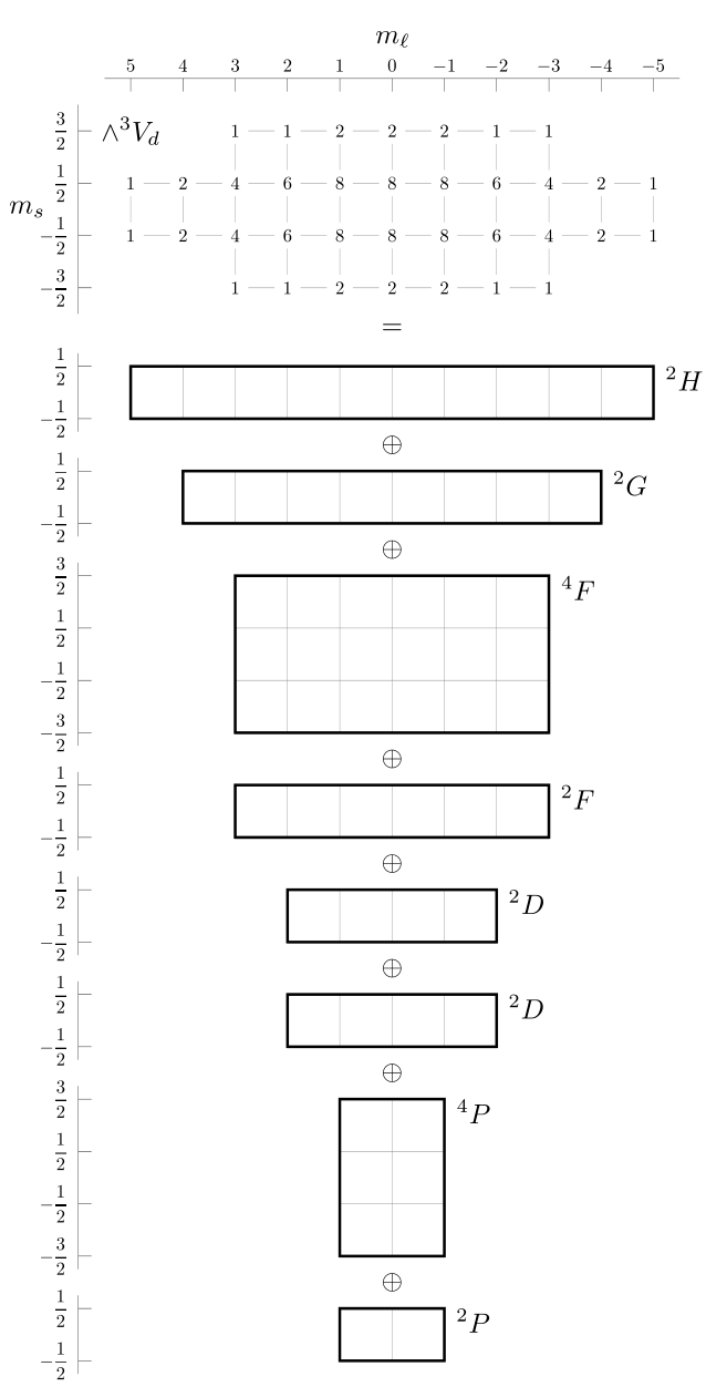
Figure 1: Algebraic decomposition of ∧3Vd\wedge^{3}V_{\mathrm{d}} into irreducible LS representation spaces Vd,3,iV_{\mathrm{d},3,i} (see equation (5)). Each of these spaces corresponds to a rectangle, matching the mℓm_{\ell} and msm_{s} quantum numbers running from ℓi,…,−ℓi\ell_{i},\dots,-\ell_{i} and si,…,−sis_{i},\dots,-s_{i}, respectively. The (ℓi,si)(\ell_{i},s_{i}) quantum numbers are displayed in common chemist’s notation as ℓ2​s+1{}^{2s+1}\ell. Superimposing all rectangles yields the multiplicities of the LzL_{z}-SzS_{z} eigenvalues in the table at the top.

The proposed algorithm (see section 2) performs the LS diagonalization implicitly, relies on the sparse matrix structure of the lowering operators L−L_{-}, S−S_{-}, and makes use of the algebraic structure of ∧nVu\wedge^{n}V_{u} as illustrated in figure 1. We present explicit tables containing decompositions of selected ∧nVu\wedge^{n}V_{u} in section 3. Given uu, the number of electrons maximizing dim(∧nVu)=(dim(Vu)n)\dim(\wedge^{n}V_{u})=\binom{\dim(V_{u})}{n} equals n=2​u+1n=2\,u+1 since dim(Vu)=2​(2​u+1)\dim(V_{u})=2\,(2\,u+1). Due to this exponential growth in uu, solving Eq. (5) for all possible nn restricts uu to the s\mathrm{s}, p\mathrm{p} and d\mathrm{d} subshells at present, and u=fu=\mathrm{f} for all n=1,…,14n=1,\dots,14 might still be attainable. On the other hand, keeping nn fixed means that dim(∧nVu)=𝒪(un)\dim(\wedge^{n}V_{u})=\mathcal{O}(u^{n}) asymptotically in uu. For a given nn the algorithm has run time

Rn​(u)=𝒪⁡(u3​n−2),R_{n}(u)=\mathcal{O}\big(u^{3n-2}\big), (7)

as derived in section 4.1. In particular, for n=2n=2, this equals 𝒪(dim(∧nVu)2)\mathcal{O}(\dim(\wedge^{n}V_{u})^{2}) (instead of 𝒪(dim(∧nVu)3)\mathcal{O}(\dim(\wedge^{n}V_{u})^{3}) for the usual diagonalization of a dense matrix).

As an alternative scenario, consider the case that we are only interested in representation spaces Vu,n,iV_{u,n,i} with ℓi\ell_{i} and sis_{i} equal (or close to) zero. As our analysis will show, this opens up the possibility of explicitly diagonalizing (1) restricted to the “central” simultaneous LzL_{z}-SzS_{z} eigenspace with eigenvalues (0,0)(0,0) for nn even and (0,12)(0,\frac{1}{2}) for nn odd, respectively. Due to symmetry, this eigenspace also has the highest dimension (denoted du,nd_{u,n}) among all simultaneous LzL_{z}-SzS_{z} eigenspaces within ∧nVu\wedge^{n}V_{u}. In section 4.2, we derive the asymptotic result

du,n≅3​dim(∧nVu)π​n​u=𝒪⁡(un−1)as ​u→∞, for fixed ​n.d_{u,n}\cong\sqrt{3}\ \frac{\dim\left(\wedge^{n}V_{u}\right)}{\pi\,n\,u}=\mathcal{O}\big(u^{n-1}\big)\quad\text{as }u\to\infty,\text{ for fixed }n. (8)

Thus, diagonalization restricted to this central eigenspace still requires 𝒪⁡(du,n3)=𝒪⁡(u3​n−3)\mathcal{O}(d_{u,n}^{3})=\mathcal{O}(u^{3n-3}) operations.

2 Algorithm

The reasoning and basic ingredients of our algorithm are as follows:

  1. 1.

    Observe that the canonical Slater determinant basis vectors of ∧nVu\wedge^{n}V_{u} are precisely the eigenvectors of both LzL_{z} and SzS_{z} acting on ∧nVu\wedge^{n}V_{u}. For example, Lz|d2d1¯d-​1⟩=(2+1−1)|d2d1¯d-​1⟩L_{z}\,\left\lvert\mathrm{d}_{2}\overline{\mathrm{d}_{1}}\mathrm{d}_{\text{-}1}\right\rangle=(2+1-1)\left\lvert\mathrm{d}_{2}\overline{\mathrm{d}_{1}}\mathrm{d}_{\text{-}1}\right\rangle and Sz|d2d1¯d-​1⟩=(12−12+12)|d2d1¯d-​1⟩S_{z}\,\left\lvert\mathrm{d}_{2}\overline{\mathrm{d}_{1}}\mathrm{d}_{\text{-}1}\right\rangle=(\frac{1}{2}-\frac{1}{2}+\frac{1}{2})\left\lvert\mathrm{d}_{2}\overline{\mathrm{d}_{1}}\mathrm{d}_{\text{-}1}\right\rangle. In particular, all simultaneous LzL_{z}-SzS_{z} eigenvalues can easily be enumerated, including multiplicities.

  2. 2.

    Let ℓmax\ell_{\max} be the largest LzL_{z} eigenvalue on ∧nVu\wedge^{n}V_{u} and WLz,maxW_{L_{z},\max} the corresponding eigenspace, as well as ψ∈WLz,max∖{0}\psi\in W_{L_{z},\max}\setminus\{0\}. Then ψ\psi must also be an 𝑳2{\boldsymbol{L}}^{2} eigenvector with eigenvalue ℓmax​(ℓmax+1)\ell_{\max}(\ell_{\max}+1). This follows from the identity

    𝑳2=Lz​(Lz+𝟏)+L−​L+{\boldsymbol{L}}^{2}=L_{z}(L_{z}+\boldsymbol{1})+L_{-}L_{+} (9)

    and the fact that L+L_{+} is zero on WLz,maxW_{L_{z},\max} since ℓmax\ell_{\max} is – by definition – the largest LzL_{z} eigenvalue. The same reasoning applies to SzS_{z} and 𝑺2{\boldsymbol{S}}^{2} restricted to WLz,maxW_{L_{z},\max}. Thus we may assume that ψ\psi is also a SzS_{z}-𝑺2{\boldsymbol{S}}^{2} eigenvector with eigenvalue ss and s⁡(s+1)s(s+1), respectively.

  3. 3.

    Starting from ψ\psi, we may span an irreducible LS representation space VψV_{\psi} by repeatedly applying the lowering operators L−L_{-} and S−S_{-}. That is, Vψ:=span⁡{ψ,L−​ψ,S−​ψ,L−​S−​ψ,…}V_{\psi}:=\mathrm{span}\{\psi,L_{-}\psi,S_{-}\psi,L_{-}S_{-}\psi,\dots\}.

  4. 4.

    We obtain all remaining irreducible representation spaces by iteratively applying steps 2 and 3 to the orthogonal complement of VψV_{\psi} in ∧nVu\wedge^{n}V_{u}.

Note that although the underlying Hilbert space is complex, all steps involve real-valued matrix representations of the operators Lz,Sz,L±,S±L_{z},S_{z},L_{\pm},S_{\pm} only. Thus, the whole algorithm can be implemented on the real numbers.

Algorithm 1 Quantum numbers of all irreducible subspaces in ∧nVu\wedge^{n}V_{u}
1:  Enumerate the simultaneous eigenvalues of LzL_{z} and SzS_{z} acting on ∧nVu\wedge^{n}V_{u}, including multiplicities, and store them in a table denoted TzT_{z}. For example, figure 1 shows the multiplicity table for ∧3Vd\wedge^{3}V_{\mathrm{d}}.
2:  i←1i\leftarrow 1
3:  while TzT_{z} contains non-zero multiplicities do
4:   Let ℓ:=ℓmax\ell:=\ell_{\max} be the greatest LzL_{z} eigenvalue in TzT_{z} with non-zero multiplicity, and let ss be a corresponding SzS_{z} eigenvalue which is maximal among all tuples (ℓmax,s)(\ell_{\max},s) in TzT_{z}.
5:   Calculate the mℓm_{\ell} and msm_{s} quantum numbers corresponding to (ℓ,s)(\ell,s), i.e., the tuples (mℓ,ms)(m_{\ell},m_{s}) for all mℓ=ℓ,…,−ℓm_{\ell}=\ell,\dots,-\ell and ms=s,…,−sm_{s}=s,\dots,-s. Decrement the multiplicity of each (mℓ,ms)(m_{\ell},m_{s}) in TzT_{z} by one.
6:   (ℓi,si)←(ℓ,s)(\ell_{i},s_{i})\leftarrow(\ell,s) (store the current quantum numbers), and increment ii.
7:  end while

The LzL_{z}-SzS_{z} quantum numbers (including multiplicities) are sufficient to calculate the (ℓi,si)(\ell_{i},s_{i}) quantum numbers in Eq. (6), see algorithm 1. Since each irreducible LS space contains exactly one vector in the “central” simultaneous LzL_{z}-SzS_{z} eigenspace with eigenvalues (0,0)(0,0) (nn even) or (0,12)(0,\frac{1}{2}) (nn odd) and multiplicity du,nd_{u,n}, there are exactly du,nd_{u,n} irreducible LS spaces.

Algorithm 2 actually performs the simultaneous diagonalization. It requires the (ℓi,si)(\ell_{i},s_{i}) tuples computed by algorithm 1.

Algorithm 2 Simultaneous diagonalization of the operators (1) on ∧nVu\wedge^{n}V_{u}, yielding the decomposition (5)
0:  Irreducible representation space quantum numbers (ℓi,si)(\ell_{i},s_{i}) as computed by algorithm 1.
1:  Partition the canonical Slater determinant basis of ∧nVu\wedge^{n}V_{u} into simultaneous LzL_{z}-SzS_{z} eigenspaces denoted Wmℓ,msW_{m_{\ell},m_{s}}. That is, Wmℓ,msW_{m_{\ell},m_{s}} is the eigenspace corresponding to eigenvalues mℓm_{\ell} and msm_{s}, respectively.
2:  for i=1,2,…i=1,2,\dots do
3:    Select a (normalized) ψi∈Wℓi,si\psi_{i}\in W_{\ell_{i},s_{i}} and span the corresponding irreducible representation space Vu,n,iV_{u,n,i} in (5) by repeatedly applying the lowering operators L−L_{-} and S−S_{-}. That is,
Vu,n,i:=span​{ψimℓ,ms}mℓ=ℓi,…,−ℓi,ms=si,…,−siwith\displaystyle V_{u,n,i}:=\mathrm{span}\left\{\psi_{i}^{m_{\ell},m_{s}}\right\}_{m_{\ell}=\ell_{i},\dots,-\ell_{i},m_{s}=s_{i},\dots,-s_{i}}\quad\text{with}
ψiℓi,si:=ψiand\displaystyle\psi_{i}^{\ell_{i},s_{i}}:=\psi_{i}\quad\text{and}
ψimℓ−1,ms:=cℓi,mℓ​L−​ψimℓ,ms,\displaystyle\psi_{i}^{m_{\ell}-1,m_{s}}:=c_{\ell_{i},m_{\ell}}L_{-}\,\psi_{i}^{m_{\ell},m_{s}},
ψimℓ,ms−1:=csi,ms​S−​ψimℓ,ms\displaystyle\psi_{i}^{m_{\ell},m_{s}-1}:=c_{s_{i},m_{s}}S_{-}\,\psi_{i}^{m_{\ell},m_{s}}
and the normalization factors cℓ,m:=(ℓ(ℓ+1)−m(m−1))−1/2c_{\ell,m}:=(\ell(\ell+1)-m(m-1))^{-1/2}.
4:   Remove the vectors spanning Vu,n,iV_{u,n,i} from any corresponding LzL_{z}-SzS_{z} eigenspace Wℓj,sjW_{\ell_{j},s_{j}} with ℓj≤ℓi\ell_{j}\leq\ell_{i} and sj≤sis_{j}\leq s_{i}. More precisely, update Wℓj,sjW_{\ell_{j},s_{j}} such that it contains the orthogonal complement of ψiℓj,sj\psi_{i}^{\ell_{j},s_{j}} in Wℓj,sjW_{\ell_{j},s_{j}}.
5:  end for

The basis vectors spanning the orthogonal complement in Wℓj,sjW_{\ell_{j},s_{j}} (line 4) are not unique. This poses a practical problem for symbolic computer algebra implementations. Namely, orthonormalizing these basis vectors can lead to a blow-up of nested squares, which is particularly unfavorable since subsequently the lowering operators (line 3) are applied to these vectors. To circumvent this difficulty, one can instead work with the unique projection matrix PjP_{j} acting on the basis vectors initially in Wℓj,sjW_{\ell_{j},s_{j}}. Then, in line 4, PjP_{j} is updated such that it spans precisely the orthogonal complement:

Pj←Pj−|ψiℓj,sj⟩⟨ψiℓj,sj|.P_{j}\leftarrow P_{j}-\big\lvert\psi_{i}^{\ell_{j},s_{j}}\big\rangle\big\langle\psi_{i}^{\ell_{j},s_{j}}\big\rvert. (10)

At the beginning of the algorithm, each PjP_{j} starts as identity matrix (on Wℓj,sjW_{\ell_{j},s_{j}}), and ends as zero matrix.

3 Example decompositions

Explicit decompositions of ∧nVf\wedge^{n}V_{\mathrm{f}} for n=1,2,3n=1,2,3 are shown in table 1. We have omitted ∧nVu\wedge^{n}V_{u}, u=s,p,du=\mathrm{s},\mathrm{p},\mathrm{d} since these are already published in [7]. The complete tables are available online, including a Mathematica implementation of the algorithm [8] which makes use of the FermiFab toolbox [9, 10]. For conciseness, only states with maximal LzL_{z} and SzS_{z} quantum numbers are displayed; applying the lowering operators L−L_{-} and S−S_{-} yields the remaining wavefunctions. Note that in general, symmetry levels can appear more than once within a many-particle subshell, e.g., Go2{}^{2}\mathrm{G}^{\mathrm{o}} in ∧3Vf\wedge^{3}V_{\mathrm{f}}. Thus, the tables are only unique up to (orthogonal) base changes of the states within the same symmetry level. The run time on a commodity laptop computer to calculate the symbolic eigenspaces is approximately 16 seconds for u=fu=\mathrm{f} and n=3n=3, and 550 seconds for u=fu=\mathrm{f} and n=4n=4.

config sym LzL_{z} Sz\mathrm{S}_{z} Ψ\Psi
∧1Vf\wedge^{1}V_{\mathrm{f}} Fo2{}^{2}\mathrm{F}^{\mathrm{o}} 33 12\frac{1}{2} |f3⟩\left\lvert\mathrm{f}_{3}\right\rangle
∧2Vf\wedge^{2}V_{\mathrm{f}} I1{}^{1}\mathrm{I} 66 00 |f3f3¯⟩\left\lvert\mathrm{f}_{3}\overline{\mathrm{f}_{3}}\right\rangle
H3{}^{3}\mathrm{H} 55 11 |f3f2⟩\left\lvert\mathrm{f}_{3}\mathrm{f}_{2}\right\rangle
G1{}^{1}\mathrm{G} 44 00 111(−3⋅|f3f1¯⟩+3⋅|f3¯f1⟩+5⋅|f2f2¯⟩)\frac{1}{\sqrt{11}}\left(-\sqrt{3}\cdot\left\lvert\mathrm{f}_{3}\overline{\mathrm{f}_{1}}\right\rangle+\sqrt{3}\cdot\left\lvert\overline{\mathrm{f}_{3}}\mathrm{f}_{1}\right\rangle+\sqrt{5}\cdot\left\lvert\mathrm{f}_{2}\overline{\mathrm{f}_{2}}\right\rangle\right)
F3{}^{3}\mathrm{F} 33 11 13(−|f3f0⟩+2⋅|f2f1⟩)\frac{1}{\sqrt{3}}\left(-\left\lvert\mathrm{f}_{3}\mathrm{f}_{0}\right\rangle+\sqrt{2}\cdot\left\lvert\mathrm{f}_{2}\mathrm{f}_{1}\right\rangle\right)
D1{}^{1}\mathrm{D} 22 00 142(5⋅|f3f-​1¯⟩−5⋅|f3¯f-​1⟩−10⋅|f2f0¯⟩+10⋅|f2¯f0⟩+23⋅|f1f1¯⟩)\frac{1}{\sqrt{42}}\left(\sqrt{5}\cdot\left\lvert\mathrm{f}_{3}\overline{\mathrm{f}_{\text{-}1}}\right\rangle-\sqrt{5}\cdot\left\lvert\overline{\mathrm{f}_{3}}\mathrm{f}_{\text{-}1}\right\rangle-\sqrt{10}\cdot\left\lvert\mathrm{f}_{2}\overline{\mathrm{f}_{0}}\right\rangle+\sqrt{10}\cdot\left\lvert\overline{\mathrm{f}_{2}}\mathrm{f}_{0}\right\rangle+2\sqrt{3}\cdot\left\lvert\mathrm{f}_{1}\overline{\mathrm{f}_{1}}\right\rangle\right)
P3{}^{3}\mathrm{P} 11 11 114(3⋅|f3f-​2⟩−5⋅|f2f-​1⟩+6⋅|f1f0⟩)\frac{1}{\sqrt{14}}\left(\sqrt{3}\cdot\left\lvert\mathrm{f}_{3}\mathrm{f}_{\text{-}2}\right\rangle-\sqrt{5}\cdot\left\lvert\mathrm{f}_{2}\mathrm{f}_{\text{-}1}\right\rangle+\sqrt{6}\cdot\left\lvert\mathrm{f}_{1}\mathrm{f}_{0}\right\rangle\right)
S1{}^{1}\mathrm{S} 00 00 17(−|f3f-​3¯⟩+|f3¯f-​3⟩+|f2f-​2¯⟩−|f2¯f-​2⟩−|f1f-​1¯⟩+|f1¯f-​1⟩+|f0f0¯⟩)\frac{1}{\sqrt{7}}\left(-\left\lvert\mathrm{f}_{3}\overline{\mathrm{f}_{\text{-}3}}\right\rangle+\left\lvert\overline{\mathrm{f}_{3}}\mathrm{f}_{\text{-}3}\right\rangle+\left\lvert\mathrm{f}_{2}\overline{\mathrm{f}_{\text{-}2}}\right\rangle-\left\lvert\overline{\mathrm{f}_{2}}\mathrm{f}_{\text{-}2}\right\rangle-\left\lvert\mathrm{f}_{1}\overline{\mathrm{f}_{\text{-}1}}\right\rangle+\left\lvert\overline{\mathrm{f}_{1}}\mathrm{f}_{\text{-}1}\right\rangle+\left\lvert\mathrm{f}_{0}\overline{\mathrm{f}_{0}}\right\rangle\right)
∧3Vf\wedge^{3}V_{\mathrm{f}} Ko2{}^{2}\mathrm{K}^{\mathrm{o}} 88 12\frac{1}{2} |f3f3¯f2⟩\left\lvert\mathrm{f}_{3}\overline{\mathrm{f}_{3}}\mathrm{f}_{2}\right\rangle
Jo2{}^{2}\mathrm{J}^{\mathrm{o}} 77 12\frac{1}{2} 12​2(3⋅|f3f3¯f1⟩+5⋅|f3f2f2¯⟩)\frac{1}{2\sqrt{2}}\left(\sqrt{3}\cdot\left\lvert\mathrm{f}_{3}\overline{\mathrm{f}_{3}}\mathrm{f}_{1}\right\rangle+\sqrt{5}\cdot\left\lvert\mathrm{f}_{3}\mathrm{f}_{2}\overline{\mathrm{f}_{2}}\right\rangle\right)
Io4{}^{4}\mathrm{I}^{\mathrm{o}} 66 32\frac{3}{2} |f3f2f1⟩\left\lvert\mathrm{f}_{3}\mathrm{f}_{2}\mathrm{f}_{1}\right\rangle
Io2{}^{2}\mathrm{I}^{\mathrm{o}} 66 12\frac{1}{2} 121(3⋅|f3f3¯f0⟩−2⋅|f3f2f1¯⟩−2⋅|f3f2¯f1⟩+22⋅|f3¯f2f1⟩)\frac{1}{\sqrt{21}}\left(3\cdot\left\lvert\mathrm{f}_{3}\overline{\mathrm{f}_{3}}\mathrm{f}_{0}\right\rangle-\sqrt{2}\cdot\left\lvert\mathrm{f}_{3}\mathrm{f}_{2}\overline{\mathrm{f}_{1}}\right\rangle-\sqrt{2}\cdot\left\lvert\mathrm{f}_{3}\overline{\mathrm{f}_{2}}\mathrm{f}_{1}\right\rangle+2\sqrt{2}\cdot\left\lvert\overline{\mathrm{f}_{3}}\mathrm{f}_{2}\mathrm{f}_{1}\right\rangle\right)
Ho2{}^{2}\mathrm{H}^{\mathrm{o}} 55 12\frac{1}{2} 16(2⋅|f3f3¯f-​1⟩−|f3f2¯f0⟩+|f3¯f2f0⟩+2⋅|f2f2¯f1⟩)\frac{1}{\sqrt{6}}\left(\sqrt{2}\cdot\left\lvert\mathrm{f}_{3}\overline{\mathrm{f}_{3}}\mathrm{f}_{\text{-}1}\right\rangle-\left\lvert\mathrm{f}_{3}\overline{\mathrm{f}_{2}}\mathrm{f}_{0}\right\rangle+\left\lvert\overline{\mathrm{f}_{3}}\mathrm{f}_{2}\mathrm{f}_{0}\right\rangle+\sqrt{2}\cdot\left\lvert\mathrm{f}_{2}\overline{\mathrm{f}_{2}}\mathrm{f}_{1}\right\rangle\right)
Ho2{}^{2}\mathrm{H}^{\mathrm{o}} 55 12\frac{1}{2} 1273(−5⋅|f3f3¯f-​1⟩−310⋅|f3f2f0¯⟩+210⋅|f3f2¯f0⟩+63⋅|f3f1f1¯⟩\frac{1}{\sqrt{273}}\left(-\sqrt{5}\cdot\left\lvert\mathrm{f}_{3}\overline{\mathrm{f}_{3}}\mathrm{f}_{\text{-}1}\right\rangle-3\sqrt{10}\cdot\left\lvert\mathrm{f}_{3}\mathrm{f}_{2}\overline{\mathrm{f}_{0}}\right\rangle+2\sqrt{10}\cdot\left\lvert\mathrm{f}_{3}\overline{\mathrm{f}_{2}}\mathrm{f}_{0}\right\rangle+6\sqrt{3}\cdot\left\lvert\mathrm{f}_{3}\mathrm{f}_{1}\overline{\mathrm{f}_{1}}\right\rangle\right.
+10⋅|f3¯f2f0⟩+25⋅|f2f2¯f1⟩)\left.+\sqrt{10}\cdot\left\lvert\overline{\mathrm{f}_{3}}\mathrm{f}_{2}\mathrm{f}_{0}\right\rangle+2\sqrt{5}\cdot\left\lvert\mathrm{f}_{2}\overline{\mathrm{f}_{2}}\mathrm{f}_{1}\right\rangle\right)
Go4{}^{4}\mathrm{G}^{\mathrm{o}} 44 32\frac{3}{2} 111(−5⋅|f3f2f-​1⟩+6⋅|f3f1f0⟩)\frac{1}{\sqrt{11}}\left(-\sqrt{5}\cdot\left\lvert\mathrm{f}_{3}\mathrm{f}_{2}\mathrm{f}_{\text{-}1}\right\rangle+\sqrt{6}\cdot\left\lvert\mathrm{f}_{3}\mathrm{f}_{1}\mathrm{f}_{0}\right\rangle\right)
Go2{}^{2}\mathrm{G}^{\mathrm{o}} 44 12\frac{1}{2} 17​5(53⋅|f3f3¯f-​2⟩+5⋅|f3f2f-​1¯⟩−35⋅|f3f2¯f-​1⟩−6⋅|f3f1f0¯⟩\frac{1}{7\sqrt{5}}\left(5\sqrt{3}\cdot\left\lvert\mathrm{f}_{3}\overline{\mathrm{f}_{3}}\mathrm{f}_{\text{-}2}\right\rangle+\sqrt{5}\cdot\left\lvert\mathrm{f}_{3}\mathrm{f}_{2}\overline{\mathrm{f}_{\text{-}1}}\right\rangle-3\sqrt{5}\cdot\left\lvert\mathrm{f}_{3}\overline{\mathrm{f}_{2}}\mathrm{f}_{\text{-}1}\right\rangle-\sqrt{6}\cdot\left\lvert\mathrm{f}_{3}\mathrm{f}_{1}\overline{\mathrm{f}_{0}}\right\rangle\right.
+6⋅|f3f1¯f0⟩+25⋅|f3¯f2f-​1⟩+210⋅|f2f2¯f0⟩+43⋅|f2f1f1¯⟩)\left.+\sqrt{6}\cdot\left\lvert\mathrm{f}_{3}\overline{\mathrm{f}_{1}}\mathrm{f}_{0}\right\rangle+2\sqrt{5}\cdot\left\lvert\overline{\mathrm{f}_{3}}\mathrm{f}_{2}\mathrm{f}_{\text{-}1}\right\rangle+2\sqrt{10}\cdot\left\lvert\mathrm{f}_{2}\overline{\mathrm{f}_{2}}\mathrm{f}_{0}\right\rangle+4\sqrt{3}\cdot\left\lvert\mathrm{f}_{2}\mathrm{f}_{1}\overline{\mathrm{f}_{1}}\right\rangle\right)
Go2{}^{2}\mathrm{G}^{\mathrm{o}} 44 12\frac{1}{2} 17​429(−186⋅|f3f3¯f-​2⟩+1610⋅|f3f2f-​1¯⟩+10⋅|f3f2¯f-​1⟩−323⋅|f3f1f0¯⟩\frac{1}{7\sqrt{429}}\left(-18\sqrt{6}\cdot\left\lvert\mathrm{f}_{3}\overline{\mathrm{f}_{3}}\mathrm{f}_{\text{-}2}\right\rangle+16\sqrt{10}\cdot\left\lvert\mathrm{f}_{3}\mathrm{f}_{2}\overline{\mathrm{f}_{\text{-}1}}\right\rangle+\sqrt{10}\cdot\left\lvert\mathrm{f}_{3}\overline{\mathrm{f}_{2}}\mathrm{f}_{\text{-}1}\right\rangle-32\sqrt{3}\cdot\left\lvert\mathrm{f}_{3}\mathrm{f}_{1}\overline{\mathrm{f}_{0}}\right\rangle\right.
−173⋅|f3f1¯f0⟩−1710⋅|f3¯f2f-​1⟩+493⋅|f3¯f1f0⟩+155⋅|f2f2¯f0⟩\left.-17\sqrt{3}\cdot\left\lvert\mathrm{f}_{3}\overline{\mathrm{f}_{1}}\mathrm{f}_{0}\right\rangle-17\sqrt{10}\cdot\left\lvert\overline{\mathrm{f}_{3}}\mathrm{f}_{2}\mathrm{f}_{\text{-}1}\right\rangle+49\sqrt{3}\cdot\left\lvert\overline{\mathrm{f}_{3}}\mathrm{f}_{1}\mathrm{f}_{0}\right\rangle+15\sqrt{5}\cdot\left\lvert\mathrm{f}_{2}\overline{\mathrm{f}_{2}}\mathrm{f}_{0}\right\rangle\right.
+156⋅|f2f1f1¯⟩)\left.+15\sqrt{6}\cdot\left\lvert\mathrm{f}_{2}\mathrm{f}_{1}\overline{\mathrm{f}_{1}}\right\rangle\right)
Fo4{}^{4}\mathrm{F}^{\mathrm{o}} 33 32\frac{3}{2} 12(|f3f2f-​2⟩−|f3f1f-​1⟩+2⋅|f2f1f0⟩)\frac{1}{2}\left(\left\lvert\mathrm{f}_{3}\mathrm{f}_{2}\mathrm{f}_{\text{-}2}\right\rangle-\left\lvert\mathrm{f}_{3}\mathrm{f}_{1}\mathrm{f}_{\text{-}1}\right\rangle+\sqrt{2}\cdot\left\lvert\mathrm{f}_{2}\mathrm{f}_{1}\mathrm{f}_{0}\right\rangle\right)
Fo2{}^{2}\mathrm{F}^{\mathrm{o}} 33 12\frac{1}{2} 16(|f3f3¯f-​3⟩+|f3f2f-​2¯⟩−|f3f2¯f-​2⟩−|f3f1f-​1¯⟩\frac{1}{\sqrt{6}}\left(\left\lvert\mathrm{f}_{3}\overline{\mathrm{f}_{3}}\mathrm{f}_{\text{-}3}\right\rangle+\left\lvert\mathrm{f}_{3}\mathrm{f}_{2}\overline{\mathrm{f}_{\text{-}2}}\right\rangle-\left\lvert\mathrm{f}_{3}\overline{\mathrm{f}_{2}}\mathrm{f}_{\text{-}2}\right\rangle-\left\lvert\mathrm{f}_{3}\mathrm{f}_{1}\overline{\mathrm{f}_{\text{-}1}}\right\rangle\right.
+|f3f1¯f-​1⟩+|f3f0f0¯⟩)\left.+\left\lvert\mathrm{f}_{3}\overline{\mathrm{f}_{1}}\mathrm{f}_{\text{-}1}\right\rangle+\left\lvert\mathrm{f}_{3}\mathrm{f}_{0}\overline{\mathrm{f}_{0}}\right\rangle\right)
Fo2{}^{2}\mathrm{F}^{\mathrm{o}} 33 12\frac{1}{2} 12​33(7⋅|f3f3¯f-​3⟩−3⋅|f3f2f-​2¯⟩−2⋅|f3f2¯f-​2⟩+3⋅|f3f1f-​1¯⟩\frac{1}{2\sqrt{33}}\left(7\cdot\left\lvert\mathrm{f}_{3}\overline{\mathrm{f}_{3}}\mathrm{f}_{\text{-}3}\right\rangle-3\cdot\left\lvert\mathrm{f}_{3}\mathrm{f}_{2}\overline{\mathrm{f}_{\text{-}2}}\right\rangle-2\cdot\left\lvert\mathrm{f}_{3}\overline{\mathrm{f}_{2}}\mathrm{f}_{\text{-}2}\right\rangle+3\cdot\left\lvert\mathrm{f}_{3}\mathrm{f}_{1}\overline{\mathrm{f}_{\text{-}1}}\right\rangle\right.
−|f3f1¯f-​1⟩−2⋅|f3f0f0¯⟩+5⋅|f3¯f2f-​2⟩−2⋅|f3¯f1f-​1⟩\left.-\left\lvert\mathrm{f}_{3}\overline{\mathrm{f}_{1}}\mathrm{f}_{\text{-}1}\right\rangle-2\cdot\left\lvert\mathrm{f}_{3}\mathrm{f}_{0}\overline{\mathrm{f}_{0}}\right\rangle+5\cdot\left\lvert\overline{\mathrm{f}_{3}}\mathrm{f}_{2}\mathrm{f}_{\text{-}2}\right\rangle-2\cdot\left\lvert\overline{\mathrm{f}_{3}}\mathrm{f}_{1}\mathrm{f}_{\text{-}1}\right\rangle\right.
+15⋅|f2f2¯f-​1⟩−2⋅|f2f1f0¯⟩−2⋅|f2f1¯f0⟩+22⋅|f2¯f1f0⟩)\left.+\sqrt{15}\cdot\left\lvert\mathrm{f}_{2}\overline{\mathrm{f}_{2}}\mathrm{f}_{\text{-}1}\right\rangle-\sqrt{2}\cdot\left\lvert\mathrm{f}_{2}\mathrm{f}_{1}\overline{\mathrm{f}_{0}}\right\rangle-\sqrt{2}\cdot\left\lvert\mathrm{f}_{2}\overline{\mathrm{f}_{1}}\mathrm{f}_{0}\right\rangle+2\sqrt{2}\cdot\left\lvert\overline{\mathrm{f}_{2}}\mathrm{f}_{1}\mathrm{f}_{0}\right\rangle\right)
Do4{}^{4}\mathrm{D}^{\mathrm{o}} 22 32\frac{3}{2} 121(10⋅|f3f2f-​3⟩−6⋅|f3f1f-​2⟩+5⋅|f3f0f-​1⟩)\frac{1}{\sqrt{21}}\left(\sqrt{10}\cdot\left\lvert\mathrm{f}_{3}\mathrm{f}_{2}\mathrm{f}_{\text{-}3}\right\rangle-\sqrt{6}\cdot\left\lvert\mathrm{f}_{3}\mathrm{f}_{1}\mathrm{f}_{\text{-}2}\right\rangle+\sqrt{5}\cdot\left\lvert\mathrm{f}_{3}\mathrm{f}_{0}\mathrm{f}_{\text{-}1}\right\rangle\right)
Do2{}^{2}\mathrm{D}^{\mathrm{o}} 22 12\frac{1}{2} 12​42(25⋅|f3f2f-​3¯⟩−5⋅|f3f2¯f-​3⟩−23⋅|f3f1f-​2¯⟩−3⋅|f3f1¯f-​2⟩\frac{1}{2\sqrt{42}}\left(2\sqrt{5}\cdot\left\lvert\mathrm{f}_{3}\mathrm{f}_{2}\overline{\mathrm{f}_{\text{-}3}}\right\rangle-\sqrt{5}\cdot\left\lvert\mathrm{f}_{3}\overline{\mathrm{f}_{2}}\mathrm{f}_{\text{-}3}\right\rangle-2\sqrt{3}\cdot\left\lvert\mathrm{f}_{3}\mathrm{f}_{1}\overline{\mathrm{f}_{\text{-}2}}\right\rangle-\sqrt{3}\cdot\left\lvert\mathrm{f}_{3}\overline{\mathrm{f}_{1}}\mathrm{f}_{\text{-}2}\right\rangle\right.
+10⋅|f3f0f-​1¯⟩+10⋅|f3f0¯f-​1⟩−5⋅|f3¯f2f-​3⟩+33⋅|f3¯f1f-​2⟩\left.+\sqrt{10}\cdot\left\lvert\mathrm{f}_{3}\mathrm{f}_{0}\overline{\mathrm{f}_{\text{-}1}}\right\rangle+\sqrt{10}\cdot\left\lvert\mathrm{f}_{3}\overline{\mathrm{f}_{0}}\mathrm{f}_{\text{-}1}\right\rangle-\sqrt{5}\cdot\left\lvert\overline{\mathrm{f}_{3}}\mathrm{f}_{2}\mathrm{f}_{\text{-}3}\right\rangle+3\sqrt{3}\cdot\left\lvert\overline{\mathrm{f}_{3}}\mathrm{f}_{1}\mathrm{f}_{\text{-}2}\right\rangle\right.
−210⋅|f3¯f0f-​1⟩+25⋅|f2f2¯f-​2⟩−5⋅|f2f1¯f-​1⟩+5⋅|f2¯f1f-​1⟩\left.-2\sqrt{10}\cdot\left\lvert\overline{\mathrm{f}_{3}}\mathrm{f}_{0}\mathrm{f}_{\text{-}1}\right\rangle+2\sqrt{5}\cdot\left\lvert\mathrm{f}_{2}\overline{\mathrm{f}_{2}}\mathrm{f}_{\text{-}2}\right\rangle-\sqrt{5}\cdot\left\lvert\mathrm{f}_{2}\overline{\mathrm{f}_{1}}\mathrm{f}_{\text{-}1}\right\rangle+\sqrt{5}\cdot\left\lvert\overline{\mathrm{f}_{2}}\mathrm{f}_{1}\mathrm{f}_{\text{-}1}\right\rangle\right.
+6⋅|f1f1¯f0⟩)\left.+\sqrt{6}\cdot\left\lvert\mathrm{f}_{1}\overline{\mathrm{f}_{1}}\mathrm{f}_{0}\right\rangle\right)
Do2{}^{2}\mathrm{D}^{\mathrm{o}} 22 12\frac{1}{2} 16​154(−145⋅|f3f2f-​3¯⟩+75⋅|f3f2¯f-​3⟩+143⋅|f3f1f-​2¯⟩−133⋅|f3f1¯f-​2⟩\frac{1}{6\sqrt{154}}\left(-14\sqrt{5}\cdot\left\lvert\mathrm{f}_{3}\mathrm{f}_{2}\overline{\mathrm{f}_{\text{-}3}}\right\rangle+7\sqrt{5}\cdot\left\lvert\mathrm{f}_{3}\overline{\mathrm{f}_{2}}\mathrm{f}_{\text{-}3}\right\rangle+14\sqrt{3}\cdot\left\lvert\mathrm{f}_{3}\mathrm{f}_{1}\overline{\mathrm{f}_{\text{-}2}}\right\rangle-13\sqrt{3}\cdot\left\lvert\mathrm{f}_{3}\overline{\mathrm{f}_{1}}\mathrm{f}_{\text{-}2}\right\rangle\right.
−10⋅|f3f0f-​1¯⟩+510⋅|f3f0¯f-​1⟩+75⋅|f3¯f2f-​3⟩−3⋅|f3¯f1f-​2⟩\left.-\sqrt{10}\cdot\left\lvert\mathrm{f}_{3}\mathrm{f}_{0}\overline{\mathrm{f}_{\text{-}1}}\right\rangle+5\sqrt{10}\cdot\left\lvert\mathrm{f}_{3}\overline{\mathrm{f}_{0}}\mathrm{f}_{\text{-}1}\right\rangle+7\sqrt{5}\cdot\left\lvert\overline{\mathrm{f}_{3}}\mathrm{f}_{2}\mathrm{f}_{\text{-}3}\right\rangle-\sqrt{3}\cdot\left\lvert\overline{\mathrm{f}_{3}}\mathrm{f}_{1}\mathrm{f}_{\text{-}2}\right\rangle\right.
−410⋅|f3¯f0f-​1⟩+65⋅|f2f2¯f-​2⟩−125⋅|f2f1f-​1¯⟩+35⋅|f2f1¯f-​1⟩\left.-4\sqrt{10}\cdot\left\lvert\overline{\mathrm{f}_{3}}\mathrm{f}_{0}\mathrm{f}_{\text{-}1}\right\rangle+6\sqrt{5}\cdot\left\lvert\mathrm{f}_{2}\overline{\mathrm{f}_{2}}\mathrm{f}_{\text{-}2}\right\rangle-12\sqrt{5}\cdot\left\lvert\mathrm{f}_{2}\mathrm{f}_{1}\overline{\mathrm{f}_{\text{-}1}}\right\rangle+3\sqrt{5}\cdot\left\lvert\mathrm{f}_{2}\overline{\mathrm{f}_{1}}\mathrm{f}_{\text{-}1}\right\rangle\right.
+125⋅|f2f0f0¯⟩+95⋅|f2¯f1f-​1⟩+96⋅|f1f1¯f0⟩)\left.+12\sqrt{5}\cdot\left\lvert\mathrm{f}_{2}\mathrm{f}_{0}\overline{\mathrm{f}_{0}}\right\rangle+9\sqrt{5}\cdot\left\lvert\overline{\mathrm{f}_{2}}\mathrm{f}_{1}\mathrm{f}_{\text{-}1}\right\rangle+9\sqrt{6}\cdot\left\lvert\mathrm{f}_{1}\overline{\mathrm{f}_{1}}\mathrm{f}_{0}\right\rangle\right)
Po2{}^{2}\mathrm{P}^{\mathrm{o}} 11 12\frac{1}{2} 12​21(6⋅|f3f1¯f-​3⟩+3⋅|f3f0f-​2¯⟩−23⋅|f3f0¯f-​2⟩−10⋅|f3f-​1f-​1¯⟩\frac{1}{2\sqrt{21}}\left(\sqrt{6}\cdot\left\lvert\mathrm{f}_{3}\overline{\mathrm{f}_{1}}\mathrm{f}_{\text{-}3}\right\rangle+\sqrt{3}\cdot\left\lvert\mathrm{f}_{3}\mathrm{f}_{0}\overline{\mathrm{f}_{\text{-}2}}\right\rangle-2\sqrt{3}\cdot\left\lvert\mathrm{f}_{3}\overline{\mathrm{f}_{0}}\mathrm{f}_{\text{-}2}\right\rangle-\sqrt{10}\cdot\left\lvert\mathrm{f}_{3}\mathrm{f}_{\text{-}1}\overline{\mathrm{f}_{\text{-}1}}\right\rangle\right.
−6⋅|f3¯f1f-​3⟩+3⋅|f3¯f0f-​2⟩−10⋅|f2f2¯f-​3⟩−6⋅|f2f1f-​2¯⟩\left.-\sqrt{6}\cdot\left\lvert\overline{\mathrm{f}_{3}}\mathrm{f}_{1}\mathrm{f}_{\text{-}3}\right\rangle+\sqrt{3}\cdot\left\lvert\overline{\mathrm{f}_{3}}\mathrm{f}_{0}\mathrm{f}_{\text{-}2}\right\rangle-\sqrt{10}\cdot\left\lvert\mathrm{f}_{2}\overline{\mathrm{f}_{2}}\mathrm{f}_{\text{-}3}\right\rangle-\sqrt{6}\cdot\left\lvert\mathrm{f}_{2}\mathrm{f}_{1}\overline{\mathrm{f}_{\text{-}2}}\right\rangle\right.
+6⋅|f2f1¯f-​2⟩+5⋅|f2f0f-​1¯⟩−5⋅|f2¯f0f-​1⟩−6⋅|f1f1¯f-​1⟩\left.+\sqrt{6}\cdot\left\lvert\mathrm{f}_{2}\overline{\mathrm{f}_{1}}\mathrm{f}_{\text{-}2}\right\rangle+\sqrt{5}\cdot\left\lvert\mathrm{f}_{2}\mathrm{f}_{0}\overline{\mathrm{f}_{\text{-}1}}\right\rangle-\sqrt{5}\cdot\left\lvert\overline{\mathrm{f}_{2}}\mathrm{f}_{0}\mathrm{f}_{\text{-}1}\right\rangle-\sqrt{6}\cdot\left\lvert\mathrm{f}_{1}\overline{\mathrm{f}_{1}}\mathrm{f}_{\text{-}1}\right\rangle\right.
−6⋅|f1f0f0¯⟩)\left.-\sqrt{6}\cdot\left\lvert\mathrm{f}_{1}\mathrm{f}_{0}\overline{\mathrm{f}_{0}}\right\rangle\right)
So4{}^{4}\mathrm{S}^{\mathrm{o}} 00 32\frac{3}{2} 17(−|f3f0f-​3⟩+2⋅|f3f-​1f-​2⟩+2⋅|f2f1f-​3⟩−|f2f0f-​2⟩+|f1f0f-​1⟩)\frac{1}{\sqrt{7}}\left(-\left\lvert\mathrm{f}_{3}\mathrm{f}_{0}\mathrm{f}_{\text{-}3}\right\rangle+\sqrt{2}\cdot\left\lvert\mathrm{f}_{3}\mathrm{f}_{\text{-}1}\mathrm{f}_{\text{-}2}\right\rangle+\sqrt{2}\cdot\left\lvert\mathrm{f}_{2}\mathrm{f}_{1}\mathrm{f}_{\text{-}3}\right\rangle-\left\lvert\mathrm{f}_{2}\mathrm{f}_{0}\mathrm{f}_{\text{-}2}\right\rangle+\left\lvert\mathrm{f}_{1}\mathrm{f}_{0}\mathrm{f}_{\text{-}1}\right\rangle\right)
Table 1: Irreducible LS eigenspace decompositions of ∧nVf\wedge^{n}V_{\mathrm{f}} for n=1,2,3n=1,2,3, see equation (5). For conciseness, the table shows states with maximal LzL_{z} and Sz\mathrm{S}_{z} quantum numbers only.

4 Complexity analysis

This section contains a derivation of Eqs. (19) and (8) in the limit of fixed electron number nn and u→∞u\to\infty.

Figure 2: Histogram plot of the LzL_{z}-SzS_{z} eigenvalue multiplicities of ∧4V8\wedge^{4}V_{8}. This is equivalent to the table in figure 1 but for u=8u=8 and n=4n=4. The probability density function approaches a normal distribution as a result of the central limit theorem for large nn; compare with proposition 1.

We first investigate the multiplicity distribution of the simultaneous LzL_{z}-SzS_{z} eigenvalues, as illustrated in figure 2. In the following, T⁡(mℓ,ms)T(m_{\ell},m_{s}) denotes the multiplicity of the simultaneous LzL_{z}-SzS_{z} eigenspace with eigenvalues (mℓ,ms)(m_{\ell},m_{s}) on ∧nVu\wedge^{n}V_{u}. We write [⋅]\left[\cdot\right] for the nearest integer function. Furthermore, fIH,nf_{\mathrm{IH},n} and fbin,n,pf_{\mathrm{bin},n,p} denote the probability density functions of the standard Irwin–Hall distribution [11, 12] (sum of nn i.i.d. U⁡(0,1)U(0,1) random variables) and the binomial distribution with parameters (n,p)(n,p), respectively.

Proposition 1.

Given a fixed integer n≥1n\geq 1, define

tu,n(xℓ,ms):=u​T​([u​xℓ],ms)dim(∧nVu),xℓ∈[−n,n],ms∈{n/2,…,−n/2}.t_{u,n}(x_{\ell},m_{s}):=\frac{u\,T(\left[u\,x_{\ell}\right],m_{s})}{\dim\left(\wedge^{n}V_{u}\right)},\quad x_{\ell}\in[-n,n],\quad m_{s}\in\left\{n/2,\dots,-n/2\right\}. (11)

Then for each msm_{s},

limu→∞tu,n​(xℓ,ms)=fLz​(xℓ)​fSz​(ms)\lim_{u\to\infty}t_{u,n}(x_{\ell},m_{s})=f_{L_{z}}\!(x_{\ell})f_{S_{z}}\!(m_{s}) (12)

uniformly in xℓx_{\ell} with

fLz​(xℓ):=12​fIH,n​(xℓ2+n2),fSz​(ms):=fbin,n,12​(ms+n2).f_{L_{z}}\!(x_{\ell}):=\frac{1}{2}\,f_{\mathrm{IH},n}\!\left(\frac{x_{\ell}}{2}+\frac{n}{2}\right),\quad f_{S_{z}}\!(m_{s}):=f_{\mathrm{bin},n,\frac{1}{2}}\left(m_{s}+\frac{n}{2}\right). (13)

In particular, fLzf_{L_{z}} and fSzf_{S_{z}} have zero mean and variances σℓ2=n/3\sigma_{\ell}^{2}=n/3 and σs2=n/4\sigma_{s}^{2}=n/4, respectively.

The factor uu in the definition of tu,nt_{u,n} ensures normalization in the sense that

∑ms∫[−n,n]tu,n(xℓ,ms)dxℓ=dim(∧nVu)−1∑ms∫[−n​u,n​u]T([mℓ],ms)dmℓ≅dim(∧nVu)−1∑mℓ,msT(mℓ,ms)=1.\begin{split}&\sum_{m_{s}}\int_{[-n,n]}t_{u,n}(x_{\ell},m_{s})\,\mathrm{d}x_{\ell}=\dim\left(\wedge^{n}V_{u}\right)^{-1}\sum_{m_{s}}\int_{[-n\,u,n\,u]}T(\left[m_{\ell}\right],m_{s})\,\mathrm{d}m_{\ell}\\ &\qquad\cong\dim\left(\wedge^{n}V_{u}\right)^{-1}\sum_{m_{\ell},m_{s}}T(m_{\ell},m_{s})=1.\end{split} (14)
Proof.

First label the basis vectors (“spherical harmonics”) spanning VuV_{u} abstractly as

Yu:={u↑,u↓,…,(−u)↑,(−u)↓}.Y_{u}:=\left\{u\!\uparrow,u\!\downarrow,\dots,(-u)\!\uparrow,(-u)\!\downarrow\right\}. (15)

Now let ψ=|φ1,…,φn⟩∈∧nVu\psi=\left\lvert\varphi_{1},\dots,\varphi_{n}\right\rangle\in\wedge^{n}V_{u} be a uniformly random Slater determinant, with φi∈Yu\varphi_{i}\in Y_{u} pairwise different. In other words, ψ\psi randomly selects nn distinct elements from YuY_{u}. As already shown in the beginning of section 2, ψ\psi is a simultaneous LzL_{z}-SzS_{z} eigenvector. To estimate the distribution (eigLz​(ψ),eigSz​(ψ))(\mathrm{eig}_{L_{z}}\!(\psi),\mathrm{eig}_{S_{z}}\!(\psi)), note that LzL_{z} and SzS_{z} just sum up the corresponding terms in ψ\psi. Thus, for example,

eigLz(|↑,↓,−↑⟩)\displaystyle\mathrm{eig}_{L_{z}}\!(\left\lvert 2\!\uparrow,1\!\downarrow,-1\!\uparrow\right\rangle) =2+1−1=2,\displaystyle=2+1-1=2, (16)
eigSz(|↑,↓,−↑⟩)\displaystyle\mathrm{eig}_{S_{z}}\!(\left\lvert 2\!\uparrow,1\!\downarrow,-1\!\uparrow\right\rangle) =12−12+12=12.\displaystyle=\tfrac{1}{2}-\tfrac{1}{2}+\tfrac{1}{2}=\tfrac{1}{2}. (17)

Observe that the error incurred by ignoring the exclusion principle goes to zero as u→∞u\to\infty due to n≪un\ll u. That is, we may replace ψ\psi by ψ~:=φ~1⊗⋯⊗φ~n∈⨂nVu\tilde{\psi}:=\tilde{\varphi}_{1}\otimes\cdots\otimes\tilde{\varphi}_{n}\in\bigotimes^{n}V_{u} with φ~i∈Yu\tilde{\varphi}_{i}\in Y_{u} i.i.d. (independent and identically distributed). Then eigLz​(ψ~)\mathrm{eig}_{L_{z}}\!(\tilde{\psi}) and eigSz​(ψ~)\mathrm{eig}_{S_{z}}\!(\tilde{\psi}) are independent as well and can be handled separately. The distribution fSzf_{S_{z}} stems directly from eigSz​(ψ~)=∑ieigSz​(φ~i)\mathrm{eig}_{S_{z}}\!(\tilde{\psi})=\sum_{i}\mathrm{eig}_{S_{z}}\!(\tilde{\varphi}_{i}). Considering eigLz​(ψ~)\mathrm{eig}_{L_{z}}\!(\tilde{\psi}), first note that the discretization error

|fLz​(xℓ)−fLz​([u​xℓ]u)|→0\left\lvert f_{L_{z}}\!(x_{\ell})-f_{L_{z}}\!\left(\frac{\left[u\,x_{\ell}\right]}{u}\right)\right\rvert\to 0 (18)

as u→∞u\to\infty since fLzf_{L_{z}} is uniformly continuous. Thus, the distribution of 1u​eigLz​(φ~i)\frac{1}{u}\,\mathrm{eig}_{L_{z}}\!(\tilde{\varphi}_{i}) approaches U⁡(−1,1)U(-1,1), and consequently, 1u​eigLz​(ψ~)=∑i1u​eigLz​(φ~i)∼fLz\frac{1}{u}\,\mathrm{eig}_{L_{z}}\!(\tilde{\psi})=\sum_{i}\frac{1}{u}\,\mathrm{eig}_{L_{z}}\!(\tilde{\varphi}_{i})\sim f_{L_{z}}. ∎

4.1 Run time

This subsection is concerned with the asymptotic run time of the main algorithm, as already stated in the introduction.

Proposition 2.

For any fixed integer n≥1n\geq 1, the run time Rn​(u)R_{n}(u) of algorithm 2 obeys

Rn​(u)=𝒪⁡(u3​n−2)R_{n}(u)=\mathcal{O}\big(u^{3n-2}\big) (19)

as u→∞u\to\infty.

Proof.

Due to the sparse matrix structure of the lowering operators L−L_{-} and S−S_{-}, each matrix multiplication in line 3 of the algorithm has linear (instead of quadratic) cost. Thus, the main computational cost stems from line 4. Denote the tuples (ℓi,si)(\ell_{i},s_{i}) after deleting duplicates by (ℓk′,sk′)(\ell^{\prime}_{k},s^{\prime}_{k}). For each simultaneous LzL_{z}-SzS_{z} eigenspace Wℓk′,sk′W_{\ell^{\prime}_{k},s^{\prime}_{k}} with dimension dk:=dim(Wℓk′,sk′)d_{k}:=\dim(W_{\ell^{\prime}_{k},s^{\prime}_{k}}), the algorithm calculates dkd_{k} orthogonal complements within Wℓk′,sk′W_{\ell^{\prime}_{k},s^{\prime}_{k}}, each of which takes 𝒪⁡(dk2)\mathcal{O}(d_{k}^{2}) operations. So in total, Rn​(u)=𝒪⁡(∑kdk3)R_{n}(u)=\mathcal{O}(\sum_{k}d_{k}^{3}). Combining this result with (12) yields the following upper bound,

Rn​(u)≲14dim(∧nVu)3∫[−n​u,n​u]u−3fLz(mℓ/u)3dmℓ∑msfSz(ms)3=14dim(∧nVu)3u−2∫ℝfIH,n(xℓ)3dxℓ∑xs=0nfbin,n,12(xs)3=𝒪⁡(u3​n−2).\begin{split}R_{n}(u)&\lesssim\frac{1}{4}\dim\left(\wedge^{n}V_{u}\right)^{3}\int_{[-n\,u,n\,u]}u^{-3}\,f_{L_{z}}(m_{\ell}/u)^{3}\,\mathrm{d}m_{\ell}\,\sum_{m_{s}}f_{S_{z}}(m_{s})^{3}\\ &=\frac{1}{4}\dim\left(\wedge^{n}V_{u}\right)^{3}u^{-2}\int_{\mathbb{R}}f_{\mathrm{IH},n}(x_{\ell})^{3}\,\mathrm{d}x_{\ell}\sum_{x_{s}=0}^{n}f_{\mathrm{bin},n,\frac{1}{2}}(x_{s})^{3}\\ &=\mathcal{O}\big(u^{3n-2}\big).\end{split} (20)

The factor 14\frac{1}{4} stems from the observation that for each kk, neither Wℓk′,−sk′W_{\ell^{\prime}_{k},-s^{\prime}_{k}}, W−ℓk′,sk′W_{-\ell^{\prime}_{k},s^{\prime}_{k}} nor W−ℓk′,−sk′W_{-\ell^{\prime}_{k},-s^{\prime}_{k}} contribute to the cost. The second line follows from a change of variables, and the third from noting that the integral and sum in the second line do not depend on uu. ∎

Taking one step further, we can now investigate the dependency of Rn​(u)R_{n}(u) on nn in more detail and evaluate the terms in the second line of (20). We obtain the following

Lemma 3.

Assume that nn is large enough such that fLzf_{L_{z}} and fSzf_{S_{z}} can be well approximated by Gaussian normal distributions with mean 00 and variances σℓ\sigma_{\ell} and σs\sigma_{s} from proposition 1. Then

Rn​(u)≲dim(∧nVu)348​π2​u2​σℓ2​σs2=dim(∧nVu)3(2​π​n​u)2.R_{n}(u)\lesssim\frac{\dim\left(\wedge^{n}V_{u}\right)^{3}}{48\pi^{2}\,u^{2}\,\sigma_{\ell}^{2}\,\sigma_{s}^{2}}=\frac{\dim\left(\wedge^{n}V_{u}\right)^{3}}{(2\pi\,n\,u)^{2}}. (21)

4.2 Dimension of the central LzL_{z}-SzS_{z} eigenspace

Let du,nd_{u,n} label the maximum dimension of any simultaneous LzL_{z}-SzS_{z} eigenspace on ∧nVu\wedge^{n}V_{u}, which is attained by the “central” eigenspace with eigenvalues (mℓ,ms)=(0,0)(m_{\ell},m_{s})=(0,0) for nn even and (0,12)(0,\frac{1}{2}) for nn odd, respectively. Thus, du,nd_{u,n} can be approximated by evaluating the right side of equation (12) at these eigenvalues. A comparison with the exact du,nd_{u,n} is shown in figure 3, which nicely illustrates the polynomial scaling in uu. As a remark, fIH,n​(n2)=2π​∫0∞sinc​(x)n​𝑑xf_{\mathrm{IH},n}(\frac{n}{2})=\frac{2}{\pi}\int_{0}^{\infty}\mathrm{sinc}(x)^{n}\,\mathrm{d}x due to the convolution theorem applied to the uniform probability density function on the interval [−1/2,1/2][-1/2,1/2].

Figure 3: Log-log plot of du,nd_{u,n} versus uu for various nn. Dots are exact values, and lines show the right side of equation (12) evaluated at (mℓ,ms)=(0,0)(m_{\ell},m_{s})=(0,0) for nn even and (0,12)(0,\frac{1}{2}) for nn odd, respectively.

To derive equation (8), we follow the same procedure as above and replace fLzf_{L_{z}} and fSzf_{S_{z}} by Gaussian normal distributions. We then set ms=0m_{s}=0 both for nn even and nn odd since 12\frac{1}{2} is small compared to nn. Plugging in (mℓ,ms)=(0,0)(m_{\ell},m_{s})=(0,0) yields

Lemma 4.

Assume that nn is large enough such that fLzf_{L_{z}} and fSzf_{S_{z}} can well be approximated by Gaussian normal distributions. Then

du,n≅dim(∧nVu)2​π​u​σℓ​σs=3​dim(∧nVu)π​n​u.d_{u,n}\cong\frac{\dim\left(\wedge^{n}V_{u}\right)}{2\pi\,u\,\sigma_{\ell}\,\sigma_{s}}=\sqrt{3}\ \frac{\dim\left(\wedge^{n}V_{u}\right)}{\pi\,n\,u}. (22)

5 Conclusions

The main principle of the algorithm is the implicit simultaneous diagonalization of the many-particle angular momentum, spin and parity operators by algebraic traversal of the LzL_{z}-SzS_{z} eigenstates in the correct order. This involves 𝒪⁡(u3​n−2)\mathcal{O}(u^{3n-2}) operations for angular subshell uu filled with nn electrons. When taking any admissible nn into account, subshells up to u=du=\mathrm{d} are feasible at present, and u=fu=\mathrm{f} for all n=1,…,14n=1,\dots,14 might still be attainable. Notably, the electronic ground state configurations found in the periodic table are precisely constructed from the atomic s\mathrm{s}, p\mathrm{p}, d\mathrm{d}, f\mathrm{f} subshells.

Acknowledgments.

I would like to thank Gero Friesecke for many helpul discussions, and DFG for financial support under project FR 1275/3-1.

References

  • [1] C. Froese Fischer, T. Brage, and P. Johnsson. Computational atomic structure: An MCHF approach. CRC Press, 1997.
  • [2] S. Fraga, J. Karwowski, and K. M. S. Saxena. Handbook of atomic data. Elsevier, 1976.
  • [3] C. W. Bauschlicher and P. R. Taylor. Benchmark full configuration-interaction calculations on H2O, F, and F-. J. Chem. Phys., 85(5):2779–2783, 1986.
  • [4] M. Chaichian and R. Hagedorn. Symmetries in quantum mechanics: from angular momentum to supersymmetry. CRC Press, 1997.
  • [5] G. Friesecke and B. D. Goddard. Explicit large nuclear charge limit of electronic ground states for Li, Be, B, C, N, O, F, Ne and basic aspects of the periodic table. SIAM J. Math. Anal., 41(2):631–664, 2009.
  • [6] G. Friesecke and B. D. Goddard. Asymptotics-based CI models for atoms: properties, exact solution of a minimal model for Li to Ne, and application to atomic spectra. Multiscale Model. Simul., 7(4):1876–1897, 2009.
  • [7] C. B. Mendl and G. Friesecke. Efficient algorithm for asymptotics-based configuration-interaction methods and electronic structure of transition metal atoms. J. Chem. Phys., 133:184101, 2010.
  • [8] C. B. Mendl. https://github.com/cmendl/irredLS, 2009–2014.
  • [9] C. B. Mendl. The FermiFab toolbox for fermionic many-particle quantum systems. Comput. Phys. Commun., 182:1327–1337, 2011.
  • [10] C. B. Mendl. FermiFab Matlab/Mathematica toolbox software, online at http://sourceforge.net/projects/fermifab, 2008–2014.
  • [11] J. O. Irwin. On the frequency distribution of the means of samples from a population having any law of frequency with finite moments, with special reference to Pearson’s type II. Biometrika, 19:225–239, 1927.
  • [12] P. Hall. The distribution of means for samples of size N drawn from a population in which the variate takes values between 0 and 1, all such values being equally probable. Biometrika, 19:240–245, 1927.