Small quench dynamics as a probe for trapped ultracold atoms

The collective behavior of ultracold atoms in optical lattices can be tuned by varying the depth of lattice potentials, thus adjusting the ratio between the strength of the on-site interaction $U$ and the hopping parameter $J$. In this manner, a quantum phase transition between a superfluid (shallow lattice) and a Mott insulator (deep lattice) can be induced [1, 2, 3]. An important feature in those experiments is the presence of a (to a good approximation) harmonic trap, which results in the coexistence of superfluid and Mott domains for a wide range of values of $U/J$ [4, 5, 6]. Experiments with a few-site resolution [7], as well as single-site resolution [8, 9], have been able to resolve the site-occupation profiles and reveal the characteristic “wedding cake” structure in which Mott plateaus are flanked by superfluid domains. This phenomenology, for sufficiently deep lattices, can be described within the Bose-Hubbard model [10, 11].

While adiabatically slow variations of the lattice potential can be used as a tuning knob for quantum phase transitions in systems of trapped atoms, quenching that potential can be utilized as a means of probing the dynamics. Using this approach, in a recent experiment on quasi-one-dimensional quantum gases in an optical lattice, it was demonstrated that quasiparticle pairs transport correlations with a finite velocity across the system, leading to an effective light cone for the quantum dynamics [12]. Another possibility is to quench the harmonic trap [13, 14, 15]. It has been recently shown theoretically that a statistical analysis of the temporal fluctuations in weak quenches can be used to study phase transitions [16, 17]. In this paper, we adapt this fluctuation analysis to examine boundaries between spatially coexisting phases in trapped systems after a quench of the trapping potential.

In optical lattice experiments in which $U/J$ is not too large, but larger than the critical value for the formation of Mott insulating domains, it is challenging to accurately determine the boundaries between insulating and superfluid regions. This because the Mott insulator may exhibit sizable fluctuations of the site occupancies so single shot measurements of the latter in an insulating plateau may not look all that different from those in the superfluid region close by. For the purpose of accurately determining the boundaries between those domains, several local compressibilities have been proposed in the literature [4, 5, 18, 19], including $\kappa_{i}:=\partial\langle\hat{n}_{i}\rangle/\partial\mu_{i}$ [4], as well as the site-occupation fluctuations $\Delta n_{i}^{2}:=\langle\hat{n}_{i}^{2}\rangle-\langle\hat{n}_{i}\rangle^{2}$ [18, 19], where $\langle\bullet\rangle$ stands for the quantum expectation value and $\mu_{i}$ is the local chemical potential at site $i$.

Here we propose the use of an out-of-equilibrium quantity, the temporal variance of the expectation values of site occupancies, as a precise indicator of boundaries between domains. $\mathcal{N}_{i}(t)=\langle\hat{n}_{i}(t)\rangle$ is the expectation value of $\hat{n}_{i}(t)$, the site-occupation operator at site $i$ and at time $t$ (in the Heisenberg picture). The temporal variance of this expectation value is given by $\Delta\mathcal{N}_{i}^{2}:=\overline{\mathcal{N}_{i}^{2}}-\overline{\mathcal{N}_{i}}^{2}$, where $\overline{\bullet}$ denotes the infinite-time average $\overline{f}=\lim_{T\to\infty}T^{-1}\int_{0}^{T}f(t)dt$. Out-of-equilibrium dynamics can be triggered by making a small, sudden change in the confining potential or the lattice depth. After such a change (referred to as a quench), the site occupation expectation values $\mathcal{N}_{i}(t)$ oscillate in time. Our numerical analysis of the temporal variance of $\mathcal{N}_{i}(t)$, and of the compressibility $\kappa_{i}$, shows that $\Delta\mathcal{N}_{i}^{2}$ has several features that make it attractive as an indicator of spatial phase boundaries. Specifically, when compared to $\kappa_{i}$, (i) the temporal variance shows a stronger divergence with system size at the boundary between domains, i.e., $\Delta\mathcal{N}_{i}^{2}\propto L^{\alpha}$ with an exponent $\alpha$ which is larger than that for $\kappa_{i}$ ($L$ is the linear system size); and (ii) $\Delta\mathcal{N}_{i}^{2}$ detects finer details in the occupation profile, which are not resolved by $\kappa_{i}$. The scaling of these quantities with system size is motivated by analytical results obtained for homogeneous systems. The scaling analysis also emphasizes the point that beyond a certain system size, the temporal variance is strictly larger than the local compressibility.

Furthermore, we discuss an experimentally feasible way to study temporal fluctuations, based on a small number of temporal sampling points. We also show that a detailed analysis of the full temporal distribution $P_{\mathcal{N}_{i}}$ of $\mathcal{N}_{i}$ reveals that deep in the incompressible region, $P_{\mathcal{N}_{i}}$ is a single peaked, approximately Gaussian, narrow distribution, whereas in the boundaries with the superfluid part $P_{\mathcal{N}_{i}}$ is a double-peaked function indicating bistability and absence of equilibration. We should stress that, in this work, by small quenches we mean that the system after the quench needs to be sufficiently close to the initial equilibrium state, so that time fluctuations of site occupancies are not exponentially small as one would expect them to be in global quenches in generic systems [20].

The exposition is organized as follows. In Sec. II, we recapitulate results for homogeneous systems and present an overview of the temporal variance $\Delta\mathcal{N}_{i}^{2}$ and of the compressibility $\kappa_{i}$. In Sec. III, we apply the proposed technique for identifying phase boundaries to (integrable) hard-core boson systems. We also investigate scaling properties of the variance, as those systems allow us to obtain exact results for very large lattice sizes. We extend this analysis to a (nonintegrable) $J$-$V$-$V^{\prime}$ system in Sec. IV, and comment on the experimental viability of this approach in Sec. V. Finally, we present our conclusions in Sec. VI.

Temporal fluctuations following a quantum quench have been studied extensively in the context of homogeneous systems [21]. Since some of these results form the motivation for our analysis of inhomogeneous systems, we briefly review relevant prior work. We consider systems initialized in the ground state of a Hamiltonian $\hat{H}_{0}=\sum_{n}E_{n}|n\rangle\langle n|$. The quantum quench is then performed by suddenly changing the Hamiltonian to $\hat{H}=\hat{H}_{0}+\delta\lambda\,\hat{B}$. For definiteness, we assume that the perturbation $\hat{B}$ is local and extensive, i.e., $\hat{B}=\sum_{i}\hat{B}_{i}$ with $\left\|\hat{B}_{i}\right\|=O(L^{0})$ in the system size $L$, where $i$ denotes sites in a lattice. At time $t$ after the quench, the system’s state is given by $|\psi(t)\rangle=\exp(-it\hat{H})|\psi(0)\rangle$ (setting $\hbar=1$). For quenches with $\delta\lambda=O(L^{0})$ and a generic observable $\hat{A}$, the expectation value $\mathcal{A}(t)=\langle\hat{A}(t)\rangle=\langle\psi(t)|\hat{A}|\psi(t)\rangle$ oscillates around an average value with fluctuations $\Delta\mathcal{A}^{2}=\overline{\langle\hat{A}(t)\rangle^{2}}-\overline{\langle\hat{A}(t)\rangle}^{2}$ that are exponentially small in the system volume ¹¹ 1 By volume $V$ we mean the total volume normalized to the unit cell, i.e., the number of elementary cells (see, e.g., Ref. [23]). In other words, $\Delta\mathcal{A}^{2}=\mathcal{O}(e^{-\alpha V})$, where $\alpha$ is a positive constant. However, if the quench amplitude $\delta\lambda$ is comparatively small [i.e., $\delta\lambda\sim O(L^{-q})$ for some exponent $q>0$ to be specified], the original state is not completely destroyed during the post quench time evolution. As a result, such quench experiments can be used to obtain information on the pre-quench state of the system.

As shown in Ref. [16], the temporal variance for such small quenches is of order $\delta\lambda^{2}$, and is given by

with $Z_{n}:=A_{0,n}B_{n,0}/\left(E_{n}-E_{0}\right)$ and the notation $A_{n,m}=\langle n|\hat{A}|m\rangle$. The subscript $B$ in $\Delta_{B}\mathcal{A}^{2}$ indicates that the variance is computed for time evolution following a quench $\delta\lambda\,\hat{B}$. A simple condition for neglecting the cubic term in Eq. (1) can be written as $\delta\lambda^{2}\chi_{F}\ll 1$, where $\chi_{F}$ is the fidelity susceptibility [24]. Using the scaling law in Ref. [25], one obtains the condition $\delta\lambda\ll\min\{L^{-d/2},L^{-1/\nu}\}$, where $\nu$ is the correlation length critical exponent.

Equation (1) shows an intriguing similarity to the zero temperature equilibrium isothermal susceptibility $\chi_{AB}$ defined by $\langle\psi\left(\delta\lambda\right)|\hat{A}|\psi\left(\delta\lambda\right)\rangle=\langle\psi\left(0\right)|\hat{A}|\psi\left(0\right)\rangle-\delta\lambda\,\chi_{AB}+O\left(\delta\lambda^{2}\right)$, where $|\psi\left(\delta\lambda\right)\rangle$ is the ground state of $\hat{H}=\hat{H}_{0}+\delta\lambda\,\hat{B}$. Indeed, we have

Moreover, using Eq. (1), we see that, to second order in $\delta\lambda$, we have $\Delta_{B}\mathcal{A}^{2}=\Delta_{A}\mathcal{B}^{2}$, where we define $\mathcal{B}(t):=\langle\hat{B}(t)\rangle=\langle\psi(t)|\hat{B}|\psi(t)\rangle$. The same duality holds for the susceptibility, i.e., $\chi_{AB}=\chi_{BA}$ for Hermitian operators $\hat{A},\,\hat{B}$.

For systems with a non-zero spectral gap $\Delta$, one can further relate susceptibilities to quantum fluctuations. One can show that $\chi_{AA}\leq(2/\Delta)\Delta A^{2}$, where $\Delta A^{2}=\langle\hat{A}^{2}\rangle-\langle\hat{A}\rangle^{2}$ is the (zero-temperature) quantum fluctuation of $\hat{A}$.

Both, quantum fluctuations and generalized susceptibilities, are commonly used indicators of critical behavior in homogeneous systems. Here, we advocate for temporal fluctuations as a superior indicator. For homogeneous systems (and extensive observables) one can show that all these quantities are extensive in gapped, non-critical, systems [26, 16]. Instead, in the critical region (defined by $\xi\gg L$) one can use scaling hypothesis to predict that the behavior at criticality is [16]:

Note that if the perturbation $\hat{B}$ is relevant, one has $d+\zeta-\Delta_{B}=1/\nu>0$ and the exponent $q$ can be written as $q=d+1/\nu-\Delta_{A}$. The above equations make it clear that the strongest divergence is exhibited by the temporal fluctuations. For simplicity, setting $\hat{A}=\hat{B}$, the exponents satisfy $2d-2\Delta_{A}<q<2q$.

We verify Eqs. (4) and (5) for a tight binding model of spinless fermions $\hat{H}_{0}=\sum_{i=1}^{L}\left[-J(\hat{f}_{i}^{\dagger}\hat{f}_{i+1}+\mathrm{H.c.})\right]$ at half filling (and periodic boundary conditions) and observable/perturbation given by $\hat{A}=\hat{B}=\sum_{j}(-1)^{i}\hat{n}_{i}$. We find that the scaling of $\chi_{AB}$ and $\Delta_{B}\mathcal{A}^{2}$ is in accordance with the predictions of Eqs. (4) and (5) with $q=1$ (see Fig. 1).

Before we discuss inhomogeneous systems, which are the ones relevant in the context of ultracold atom experiments, we would like to clarify how the local compressibility $\kappa_{i}$ relates to the observables introduced so far. Straightforwardly, we realize that $\kappa_{i}=\chi_{AA}$ with $\hat{A}=\hat{n}_{i}$, whereas $\mathcal{N}_{i}(t):=\langle\hat{n}_{i}(t)\rangle$ and its (temporal) variance $\Delta_{B}\mathcal{N}_{i}^{2}$ are the dynamical counterparts. We focus on a small perturbation of the strength of a trapping potential of the form $\hat{B}=L^{-2}\sum_{i}(i-i_{0})^{2}\hat{n}_{i}$. Here $i_{0}$ is the location of the trap center, and the potential is normalized by $L^{2}$ to ensure extensivity of the Hamiltonian. (In principle, other quenches are clearly possible in which the system is perturbed by varying different parameters, e.g., the lattice depth.) Advocating a local density approximation, one can assume that a very large trapped system can be divided into extensive regions, where each region can be considered approximately homogeneous. In this case, the scaling prediction for the temporal variance of the site occupations, is

with a new scaling exponent $\gamma$. According to Eqs. (3)–(5), we expect this exponent $\gamma$ to be larger than the corresponding ones for the compressibility and site-occupation fluctuations.

As a first example for the proposed analysis, let us explore how to detect spatial boundaries between coexisting phases in an integrable model, where we can perform numerical simulations for very large systems. This also allows us to perform a finite-size scaling analysis to compare the divergence of the temporal fluctuations with that of the compressibility, demonstrating that the temporal variance exhibits a stronger divergence at the boundary between domains.

We examine a quantum system of hard-core bosons in one dimension described by the Hamiltonian

which can be thought of as the limit $U/J\rightarrow\infty$ of the Bose-Hubbard model [27]. In Eq. (6), $\hat{b}_{i}^{\dagger}$ ($\hat{b}_{i}$) is the creation (annihilation) operator of a hard-core boson at site $i$, $\hat{n}_{i}=\hat{b}_{i}^{\dagger}\hat{b}_{i}$, and $g_{i}$ describes a harmonic confining potential, with $g_{i}=L^{-2}(i-L/2+\epsilon)^{2}$. The trap is shifted off-center by a small amount $\epsilon$ to remove degeneracies in the energy levels and gaps of the Hamiltonian [see the discussion of Eq. (7)]. We initialize the system in a ground state $|\Psi(0)\rangle$ of a lattice with $L$ sites and $N$ hard-core bosons. After performing a sudden quench on the trap potential, $\lambda\rightarrow\lambda+\delta\lambda$ at time $t=0$, the system evolves unitarily as $|\Psi(t)\rangle=\exp(-i\hat{H}t)|\Psi(0)\rangle$. The post-quench Hamiltonian is given by $\hat{H}=\hat{H}_{0}+\delta\lambda\,\hat{B}$. The hard-core boson Hamiltonian (6) can be mapped onto a Hamiltonian quadratic in fermion operators $\hat{f}_{i}^{\dagger}$ and $\hat{f}_{i}$ through the Jordan-Wigner transformation [27]. From that transformation, it follows that the site occupations of hard-core bosons and spinless fermions are identical. The fermionic Hamiltonian can be written as $\hat{H}=\sum_{i,j}\hat{f}_{i}^{\dagger}M_{i,j}\hat{f}_{j}$ with $M_{i,j}=-J(\delta_{i,j+1}+\delta_{i,j-1})+(\lambda+\delta\lambda)g_{i}\delta_{i,j}$. The noninteracting character of the latter system allows one to write temporal fluctuations of site occupations (and in fact of any quadratic observable in the fermions) in terms of one-particle quantities alone. Consider the general observable $\hat{X}=\sum_{i,j}\hat{f}_{i}^{\dagger}\Gamma_{i,j}\hat{f}_{j}$. One can show that $\langle\Psi(t)|\hat{X}|\Psi(t)\rangle=\mathcal{X}(t)=\mathrm{tr}(\hat{X}e^{-it\hat{H}^{\prime}}\hat{\rho}_{0}e^{it\hat{H}^{\prime}})=\mathrm{tr}(\Gamma e^{-itM}Re^{itM})$ where $R$ is the covariance matrix of the initial state $\hat{\rho}_{0},$ i.e., $R_{i,j}=\mathrm{tr}(\hat{\rho}_{0}\hat{f}_{j}^{\dagger}\hat{f}_{i})$ (note that the initial state does not necessarily need to be Gaussian). Let the one-particle Hamiltonian $M$ have the spectral representation $M=\sum_{k}\Lambda_{k}|k\rangle\langle k|$ ($|k\rangle$ are one the particle eigenfunctions). Defining $F_{k,q}=\langle k|\Gamma|q\rangle\langle q|R|k\rangle$ where $\Gamma,\,R$ are one-particle operators, the temporal variance of $\mathcal{X}$ is then given by

Note that Eq. (1) holds for sufficiently small $\delta\lambda$ and relies on the assumption of a non-degenerate many-body spectrum. Equation (7), on the other hand, relies on the assumption of non-resonant conditions for the one-particle spectrum [28, 23], which has been verified in our numerical calculations (for $\epsilon\neq 0$). To compute the variance of the site occupations, we take $\mathcal{X}=\mathcal{N}_{i}$ with $\Gamma_{x,y}^{(i)}=\delta_{i,x}\delta_{i,y}$.

Results of our numerical simulations are shown in Fig. 2, where the site occupations are plotted along with the two measures of local critical behavior we wish to compare here. Clearly both quantities are able to distinguish the superfluid regions from the insulating plateau at the trap center. The local compressibility $\kappa_{i}$ vanishes in the plateau (band insulating) regions where the state is close to $|1,1,\ldots,1\rangle$ (trap center) and near the trap boundaries with state $|0,0,\ldots,0\rangle$. Also, $\kappa_{i}$ is roughly constant in the superfluid region. In contrast, $\Delta\mathcal{N}_{i}^{2}$ fluctuates strongly within the superfluid regime, displaying sharp peaks delineating the insulating regime from its surroundings. A closer look at the site occupation profiles [Fig. 2(b)] reveals that, due to the finite size of the system studied (which will also be the case in experiments), the site occupations at the boundary between insulating and superfluid domains change in a stepwise fashion. $\Delta\mathcal{N}_{i}^{2}$ displays clear signatures of the presence of such steps in the site occupation profiles, while they are barely reflected in $\kappa_{i}$.

More importantly, a finite-size scaling analysis reveals that the maxima of $\Delta\mathcal{N}_{i}^{2}$ diverge much more rapidly with system size than the maxima of $\kappa_{i}$ . We first verified that the size $\ell$ of the intermediate region between the two band insulator states scales as $\ell\sim L/c$ with $c\approx 4$. A fit to numerical data [see Fig. 2(d)] reveals power-law dependencies on system size $L$ (or equivalently, on $\ell$)

The scaling seen in Fig. 2(d) makes apparent that, beyond some system size (that will depend on the Hamiltonian parameters), the signal given by $\Delta\mathcal{N}_{i}^{2}$ will exceed that of $\kappa_{i}$. This means that the boundaries between domains can be determined with higher confidence using the temporal measure, provided the systems are not too small.

In general, insulating states realized in experiments exhibit nonzero quantum fluctuations of the site occupancies. This is to be contrasted to the quantum fluctuations of the site occupancies in the band insulating phases of Hamiltonian (6), which are always zero. In order to address what happens in the presence of nonzero quantum fluctuations of the site occupancies, while still retaining the advantages of dealing with models mappable to noninteracting ones, we add a staggered potential to Eq. (6) and consider

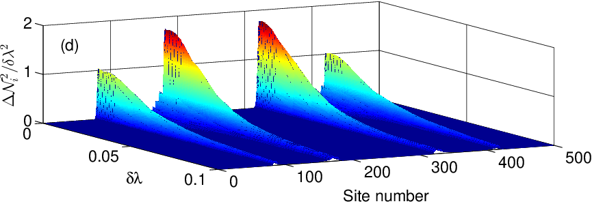
The properties of systems which such a Hamiltonian have been previously studied for spinless fermions [29] and hard-core bosons [30]. The ground state displays site-occupation fluctuations within the insulating phase with average site occupancy of 1/2. Those fluctuations vanish as $V_{0}\rightarrow\infty$, in which case the insulator becomes a product state of the form $|0,1,0,\ldots,1,0\rangle$. Accordingly, we plot all quantities in Fig. 3(a) averaged over (two site) unit cells. As seen in Fig. 3(a), for this model and the parameters chosen, the insulating plateau in the center of the trap is larger relative to the size of the superfluid domains than the one in the absence of the staggered potential. Nonetheless, the superfluid domains are clearly identifiable using $\Delta\mathcal{N}_{i}^{2}$ and $\kappa_{i}$ (notice that $\kappa_{i}$ is nonzero also in the insulating domain). Studying the finite-size scaling of the maximum of both quantities, we find the temporal variance and compressibility scaling to be,

[see Fig. 3(c)], respectively. Therefore the same conclusions hold regarding better detectability of spatial phase boundaries using $\Delta\mathcal{N}_{i}^{2}$ for sufficiently large system sizes. Interestingly, we have found that the systems sizes for which $\Delta\mathcal{N}_{i}^{2}$ starts to give a stronger signal than $\kappa_{i}$ are larger in the presence than in the absence of the staggered potential. This results from having nonzero charge fluctuations in the insulator in the center of the trap.

The dependence of the normalized temporal variance $(\Delta\mathcal{N}_{i}^{2}/\delta\lambda^{2}$) on the quench amplitude $\delta\lambda$ is depicted in Fig. 2(c) for the Hamiltonian in Eq. (6). As expected, the normalized temporal variance decays for increasing $\delta\lambda$, following a linear regime $(\Delta\mathcal{N}_{i}^{2}\propto\delta\lambda^{2}$) for small quenches ($\delta\lambda<1/L^{2}$).

In order to show that the proposed approach works beyond integrable Hamiltonians such as the ones analyzed in the previous section, here we consider a nonintegrable model. We should stress that the exponential increase of the Hilbert space with system size severely restricts the system sizes that can be studied numerically. We focus on a system consisting of hard-core bosons with nearest and next-nearest interactions (a $J$-$V$-$V^{\prime}$ model) in the presence of a harmonic trap, described by the Hamiltonian

Note that, in order to maximize the size of insulating and superfluid domains, in Eq. (13) we only consider one half of what would be the harmonic trap in an experiment.

In the absence of a trap, the phase diagram of Hamiltonian (13) has been studied using the density matrix renormalization group technique [31]. The competition between nearest-neighbor and next-nearest-neighbor interactions generates four phases: two charge-density-wave insulator phases, a superfluid (Luttinger-liquid) phase, and a bond-ordered phase. In the presence of a trap, and for a suitable choice of the parameters, the same four phases can be observed. We focus our analysis on a parameter regime where the system exhibits a charge density wave of type one (CDW-I) in the center of the trap, which is surrounded by a superfluid phase. The site occupations in the CDW-I phase are similar to those in the presence of the superlattice potential analyzed in the previous section, when the average site occupation per unit cell is 1/2 (see Fig. 4). In contrast to the superlattice case, the CDW-I phase here is not due to the presence of a translationally symmetry breaking term but is stabilized by the presence of interactions. There are two other phases that have larger unit cells, consisting of 4 sites for CDW-II and 3 sites for bond-order. The CDW-I phase is the best suited for our purposes because we are able to observe several unit cells that exhibit its expected properties.

In Fig. 4(a), we show results for a site-occupation profile exhibiting a CDW-I plateau surrounded by a small superfluid domain. In the same figure one can see that, at the edge of the CDW-I plateau, the local compressibility $\kappa_{i}$ exhibits a much weaker signal than the temporal fluctuations $\Delta\mathcal{N}_{i}^{2}$. (Note that we used multiplicative factors to enhance $\kappa_{i}$ and reduce $\Delta\mathcal{N}_{i}^{2}$ so that both measures can appear on the same scale). Also, notice that $\kappa_{i}$ does not vanish in the CDW-I plateau, which exhibits nonzero site occupation fluctuations. Since calculations for larger systems are prohibitively large, a finite-size scaling analysis of the observables is not possible here. Nonetheless, from Fig. 4(a), it is evident that the temporal variance is a better indicator of the interface between domains than the local compressibility. In fact, compared to the integrable systems considered in the preceding section, the advantage of using $\Delta\mathcal{N}_{i}^{2}$ over $\kappa_{i}$ to identify interfaces between domains is enhanced, especially taking into account the small system sizes considered here.

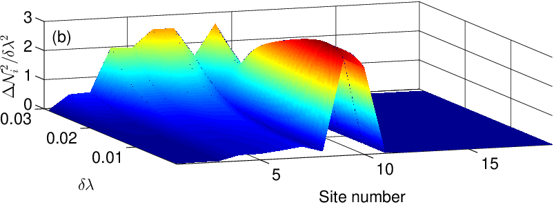
In Fig. 4(b), we plot $\Delta\mathcal{N}_{i}^{2}/\delta\lambda^{2}$ vs $\delta\lambda$. Similarly to the results in the previous section, we notice a decrease in the peak height with increasing $\delta\lambda$, following a linear regime $(\Delta\mathcal{N}_{i}^{2}\propto\delta\lambda^{2}$) at small $\delta\lambda$. For $\delta\lambda\gtrsim 0.2$, a qualitatively different behavior sets in. This is because the CDW-I domain is destroyed by the final trap and an $n=1$ Mott insulating domain appears at the potential minimum of the trap. The latter domain gives rise to a large temporal variance of the site occupations at its end, which is located in sites that were formerly in the CDW-I regime.

We now go beyond the second moment analysis presented so far and examine the full probability distribution $P_{i}(x)$ of the random variable $\mathcal{N}_{i}(t)$ equipped with the time average measure $\overline{\bullet}$. Based on the results for homogeneous systems [17, 16], we expect $P_{i}(x)$ to be a single peaked, approximately Gaussian, narrow distribution for sites $i$ deep in the (gapped) insulating regime. On the contrary, $P_{i}(x)$ is predicted to be a double peaked distribution with a relatively large variance for (critical) interface sites $i$. In a limiting, somewhat simplified case, $P_{i}(x)$ can be approximated by a two parameter distribution $P_{i}(x)=1/\left(\pi\sqrt{2\Delta\mathcal{N}_{i}^{2}-(x-\overline{\mathcal{N}_{i}})^{2}}\right)$ [17].

In Fig. 5(a), we show the distribution $P_{i}(x)$ for sites near the interface separating the insulating and superfluid regions. For sites $i$ deep in the insulating region [Fig. 5(b)], the site occupations fluctuate about one unique central value, resulting in a singly-peaked distribution function. This signifies measure concentration, indicating local equilibration in the finite system considered here [Fig. 5(c)]. In contrast, as one moves closer to the interface [Fig. 5(d)], the expectation values of observables can be approximated as [17]

with the remaining terms being negligible (the constants $\mathcal{A}_{1,2}$ depend on the initial state, evolution Hamiltonian and first excited states, see [17] for details). The probability distribution then develops peaks at $\overline{\mathcal{A}(t)}\pm||\mathcal{A}_{1}|-|\mathcal{A}_{2}||$ and a relatively large variance [17]. This bistability indicates a lack of measure concentration and a breakdown of local equilibration [see Fig. 5(e)].

So far we assumed that the expectation value $\mathcal{A}(t_{j})=\langle A(t_{j})\rangle$ could be determined exactly for various times $t_{j}$. In this section, we take a deeper look at the issue of estimating the temporal variance $\Delta\mathcal{A}^{2}$ using measurement data, keeping in mind ultracold atom experiments. In these experiments, one typically obtains information about site occupations by taking a “snapshot” of the system [8, 9] at a given time $t_{j}$ after the quench. In that case, the observable of interest is the on-site occupation number. We keep our discussion general so that it can be applied to any observable. The expectation value $\mathcal{A}(t_{j})=\langle A(t_{j})\rangle$ can be estimated by performing $N_{S}$ measurements of $A$ after the same amount of time $t_{j}$ after the quench. When $A$ is compactly supported [for Fermions $\hat{n}_{i}(t_{j})$ is actually Bernoulli distributed] the error in estimating $\mathcal{A}(t_{j})$ decreases exponentially with $N_{S}$ as a consequence of the Chernoff bound. One strategy to estimate the temporal variance would be to take $N_{S}$ sufficiently large such that $\mathcal{A}(t_{j})$ can be obtained with the desired precision. One then needs to repeat the above procedure at $N_{T}$ different times $\{t_{1},t_{2},\ldots,t_{N_{T}}\}$ where $t_{i}\in[0,T]$ to estimate the temporal variance²² 2 The question about how large should be $T$ to have $\Delta\mathcal{A}_{T}^{2}\approx\Delta\mathcal{A}^{2}$ has been addressed in [34]. Typically taking $T$ to be one or two revival times gives very accurate results. The revival time is the time required by excitations to travel the length of the system, and is hence proportional to the linear size $L$ [34]. The proportionality constant is a time-scale which is of the order of the tunneling time $\hbar/J$. . As a result, a total of $N_{S}N_{T}$ measurement are required (in principle $N_{s}$ may depend on $j$, but we do not consider this generalization here). However this may not be the best strategy to obtain the temporal variance $\Delta\mathcal{A}^{2}$. In practice one wants to minimize the total number of measurements.

In order to design better strategies, we look deeper into the measurement problem in our out-of-equilibrium setting. We recall it here for clarity: the system is prepared, $N_{S}N_{T}$ times, in the same initial state $\rho_{0}$ at time $t=0$ and allowed to evolve unitarily thereafter with the same Hamiltonian parameters. Let us denote with $A_{p}(t_{j})$ the result of the $p$-th measurement of $A$ performed at time $t_{j}$, $p=1,\ldots,N_{S}$, $j=1,\ldots,N_{T}$ (i.e., one of the eigenvalues of $A$). The random variables $A_{p}(t_{j})$ at different times are independent but not identically distributed (as opposed to measurements performed in equilibrium, in which case they are identically distributed).

In the language of statistics, what we would like to build is a consistent estimator of the temporal variance $\Delta\mathcal{A}^{2}$. A consistent estimator is a method to obtain a given quantity with the property that, as the number of data point increases, the estimator converges to the actual parameter we are trying to estimate (see e.g. Ref. [33]). In our case the data points are the random variables $A_{p}(t_{j})$. The quantum expectation value $\mathcal{A}(t_{j})=\langle A(t_{j})\rangle$ is estimated using $N_{S}$ measurements by

which converges to $\mathcal{A}(t_{j})$ in the large $N_{S}$ limit. We now define the following estimator $v$ for the the temporal variance of $A$:

Using $\mathsf{E}[\bullet]$ to denote expectation value over all the $N_{S}N_{T}$ independent measurements, we find,

We still have to specify how to choose the $N_{T}$ times. If we pick the times randomly with uniform distribution in $[0,T]$ and denote with$\mathsf{T}[\bullet]$ the corresponding time average operation (i.e., $\mathsf{T}$ averages uniformly over all $N_{T}$ independent times $t_{j}$), we obtain

where we indicated $\overline{f(t)^{T}}=T^{-1}\int_{0}^{T}f(t)dt$. We see that in the limit $N_{S},N_{T}\rightarrow\infty$, the expectation value of this estimator tends to the exact variance $\overline{(\mathcal{A}^{2})^{T}}-\left(\overline{\mathcal{A}{}^{T}}\right)^{2}=:\Delta\mathcal{A}_{T}^{2}$. This means that $v$ is an asymptotically unbiased estimator, i.e., when the number of measurement increases the estimator converges to the exact temporal variance. Furthermore, we have numerically checked that $v$ is also a consistent estimator, meaning that the error on $v$, encoded in $\mathsf{var}[v]=\mathsf{T}[\mathsf{E}[v^{2}]]-\mathsf{T}[\mathsf{E}[v]]^{2}$, tends to zero as the number of measurements increases. In Fig. 6(b), we show that $\mathsf{var}[v]\sim N_{T}^{-1}$.

We now show the feasibility of this approach for distinguishing different domains in trapped systems. We perform numerical experiments on the Hamiltonian in Eq. (13). According to our general recipe, we perform a small quench of the trapping potential and measure the occupation number at each site during the following time evolution. In this case, the observable is the site occupation $A=\hat{b}_{i}^{\dagger}\hat{b}_{i}$ and we use $v_{i}$ to denote the corresponding temporal variance estimated according to Eq. (15) for $i=1,\ldots,L$. As mentioned earlier, $A_{p}(t_{j})$ is the result of the $p$-th measurement of $A$ at time $t_{j}$. In our numerical experiments, this is obtained by randomly generating one of the eigenvalues of $A$ ($0$ or $1$ for $A=\hat{b}_{i}^{\dagger}\hat{b}_{i}$) with probabilities given by the Born rule.

In figure 6(a), we show a typical realization of $v_{i}$ obtained taking $N_{T}=10$ and $N_{S}=3$, for a total of $30$ measurements. One can compare Fig. 6 with Fig. 4(a), where the exact variance is plotted for the same parameters. Clearly, the maxima at sites $9,10$ in Fig. 6(a) predicts a transition region in agreement with that in Fig. 4(a). Still, we are primarily interested in the efficacy of $v_{i}$ in locating the boundary between coexisting phases. In other words, we are interested in knowing whether the position of the maxima of $v_{i}$ coincides with that of the exact variance [sites 9 and 10 as seen in in Figs. 4 and 6(a)]. To this end, we compute the probability $p_{M}(N_{T})=\mathrm{Prob}(\arg\max_{i}\{v_{i}\}\in\{9,10\})$ as a function of the number of measurements $N_{T}$. $p_{M}(N_{T})$ is plotted in Fig. 6(c) as a function of $N_{T}$ for different $N_{s}$. We observe that the estimator defined in Eq. (15) allows us to locate the boundary with a $90\%$ accuracy, using a total of around 40 measurements. These findings suggest that temporal fluctuations can be used to efficiently locate critical boundaries in experiments.

We have studied various trapped systems whose ground states exhibit coexistence of insulating and superfluid domains, as relevant to ultracold atom experiments in optical lattices. An analysis of the time evolution of the site occupations $\mathcal{N}_{i}$, following a small quench of the trapping potential, allowed us to show that the temporal variance of $\mathcal{N}_{i}$ can be used as an accurate tool to locate boundaries between domains. We found that the temporal variance of $\mathcal{N}_{i}$ at those boundaries exhibits a power law scaling with system size with an exponent that is greater than the one of a previously proposed local compressibility.

Furthermore, we performed a binning analysis to explicitly study the temporal probability distribution of site occupancies. Such a temporal distribution gives the probability of observing a given value of the site occupation in a large observation time-window $[0,T]$. We observed that the distributions are sharply peaked and approximately Gaussian for sites that are deep in the insulating phase, while sites at the interface display a bimodal distribution, i.e., are characterized by a lack of measure concentration. We further analyzed the feasibility of our approach from an experimental point of view. We found that since we are interested in general features of the temporal variance profile (presence of peaks at phase interfaces), rather than the exact statistics of $\mathcal{N}_{i}$, sample variances obtained using small number of measurements (around 40 for a system with $19$ sites and $5$ particles) are sufficient for locating phase boundaries with high probability.